


ABSTRACT
Pulsating low-mass white dwarf (WD) stars are WDs with stellar masses between 0.30 and 0.45 M⊙ that show photometric variability due to gravity-mode pulsations. Within this mass range, they can harbour both a helium core and hybrid core, depending if the progenitor experienced helium-core burning during the pre-WD evolution. SDSS J115219.99+024814.4 is an eclipsing binary system where both components are low-mass WDs, with stellar masses of 0.362 ± 0.014 M⊙ and 0.325 ± 0.013 M⊙. In particular, the less-massive component is a pulsating star, showing at least three pulsation periods of ∼1314, ∼1069, and ∼582.9 s. This opens the way to use asteroseismology as a tool to uncover its inner chemical structure, in combination with the information obtained using the light-curve modelling of the eclipses. To this end, using binary evolutionary models leading to helium- and hybrid-core WDs, we compute adiabatic pulsations for ℓ = 1 and ℓ = 2 gravity modes with Gyre. We found that the pulsating component of the SDSS J115219.99+024814.4 system must have a hydrogen envelope thinner than the value obtained from binary evolution computations, independently of the inner composition. Finally, from our asteroseismological study, we find a best-fitting model characterized by T|$_{\rm eff}=10\,917$| K, M = 0.338 M⊙, and MH = 10−6 M⊙ with the inner composition of a hybrid WD.
1 INTRODUCTION
White dwarfs (WDs) are the most common endpoint of stellar evolution. All stars with initial masses below 7−12 M⊙ (e.g. Garcia-Berro, Isern & Hernanz 1997; Woosley & Heger 2015; Lauffer, Romero & Kepler 2018), representing more than 95 per cent of the stars in the Milky Way, will end their lives as WDs. The WD population can be divided into hydrogen (H)-rich atmosphere objects (DA), that correspond to more than 85 per cent of all WDs, and H-deficient objects (non-DA), which show no H in their atmospheres (see Fontaine & Brassard 2008; Althaus et al. 2010a).
For H-atmosphere WDs the mass distribution peaks at ∼0.6 M⊙, which represents |$\sim\!84 {{\ \rm per\ cent}}$| of the total sample (Kepler et al. 2007; Kepler et al. 2015), exhibiting also a high- and a low-mass components. The low- and high-mass WDs are most likely the result of close binary evolution, where mass transfer and mergers commonly occur.
The low-mass tail in the DA mass distribution peaks at ∼0.39 M⊙ and extends to stellar masses <0.45 M⊙. WDs with masses <∼0.30 M⊙ can only be formed through mass transfer in close binary systems, since single star evolution is not able to form such remnants in the Hubble time (Kilic, Stanek & Pinsonneault 2007; Istrate et al. 2016; Pelisoli & Vos 2019). These objects are known as extremely low-mass white dwarfs (ELMs). Low-mass WDs are stars with stellar masses in the range of 0.30 ≤ M/M⊙ ≤ 0.45. In addition to the binary formation channel, these objects could also form as a result of strong mass-loss episodes during giant stages for high-metallicity progenitors. Noteworthy, low-mass WDs can harbour either a pure helium (He) core (e.g. Panei et al. 2007; Althaus, Miller Bertolami & Córsico 2013; Istrate, Tauris & Langer 2014; Istrate et al. 2016) or a hybrid core, composed of He, carbon (C), and oxygen (O; e.g. Iben & Tutukov 1985; Han, Tout & Eggleton 2000; Prada Moroni & Straniero 2009; Zenati, Toonen & Perets 2019).
Probably the only way to probe the inner chemical composition in detail is through the pulsation-period spectrum observed in variable stars. Each pulsation mode propagates in a specific region providing information on that particular zone, where its amplitude is maximum (Tassoul, Fontaine & Winget 1990). Thus, we can perform an asteroseismic study, where we compare the observed periods with the theoretical period spectrum, computed using representative models, to uncover the inner stellar structure (see e. g. Romero et al. 2012, 2019).
There are currently several families of pulsating WDs that can be found in specific ranges of effective temperature and surface gravity. They show g-mode non-radial pulsations with periods range from minutes to a few hours and variation amplitudes of millimag. The excitation mechanism acting on pulsating WDs is a combination of the κ-mechanism, driven by an opacity bump due to partial ionization of the main element in the outer layers (Dolez & Vauclair 1981; Winget et al. 1982), and the γ-mechanism, related to the effect of a small value of the adiabatic exponent in the ionization zone (Brickhill 1991; Goldreich & Wu 1999).
The location of the different classes in the Kiel diagram is depicted in Fig. 1. At high effective temperatures we find the GW Vir stars, with C/O atmospheres, followed by He-rich atmosphere V777 Her and the C-rich atmosphere DQV. Finally, the H-envelope pulsating WDs, known as ZZ Ceti stars, are located at lower effective temperatures. For lower log (g), we find the pulsating low-mass WDs, and the ELMs along with their progenitors, the pre-ELMs. Even though the group of pulsating ELMs is considered a class on its own, their instability strip is an extension of the ZZ Ceti instability strip to lower surface gravities, as can be seen from Fig. 1.
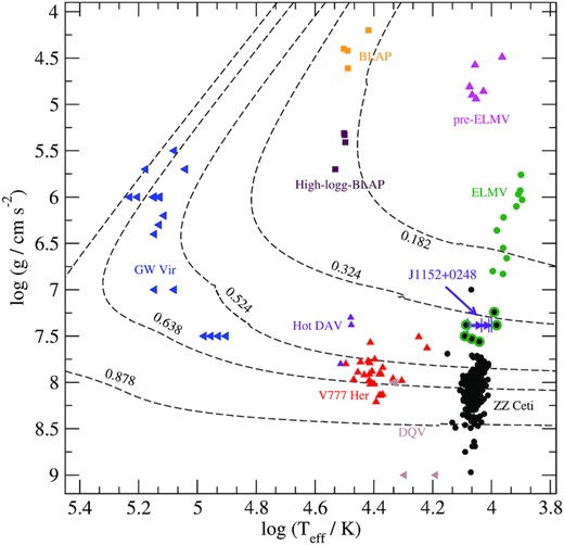
The classes of pulsating WDs. The data were extracted from Fontaine & Brassard (2008), Bognar & Sodor (2016), Pietrukowicz et al. (2017), Córsico et al. (2019), Romero et al. (2019), and Kupfer et al. (2019). For reference, we include theoretical WD sequences with C/O core and masses of 0.878, 0.638, and 0.524 M⊙ (Romero, Campos & Kepler 2015) and He-core with stellar mass of 0.324 and 0.182 M⊙ (Istrate et al. 2016). The different symbols indicate the element related to the excitation mechanism: H (circles), He (triangle-up), C and/or O (triangle-left), and iron peak elements (squares). The known variable low-mass WDs are indicated with a surrounding green circle. The position of J115219.99+024814.4 is depicted with a triangle-right, with the atmospheric parameters taken from Parsons et al. (2020; see Table 1 for details).
There are 11 pulsating ELMs known to date (green dots in Fig. 1, Hermes et al. 2013a, b; Bell et al. 2015, 2017; Kilic et al. 2015; Pelisoli et al. 2018). The pulsating ELMs are characterized by periods in the range of |$100{-}6\,300$| s, effective temperatures of |$7\,800{-}10\,000$| K, and an H-dominated surface composition (Córsico et al. 2019). In addition, there are 10 objects in the literature with stellar masses within the range 0.30 ≤ M/M⊙ ≤ 0.45 (black-green dots in Fig. 1) that show photometric variability with periods between 200 and 1300 s (Bognar & Sodor 2016; Fuchs 2017; Su et al. 2017; Rowan et al. 2019). For four of them, the uncertainties in the atmospheric parameters are quite large, leading to an uncertainty in stellar mass of 0.1–0.4 M⊙ (Su et al. 2017; Rowan et al. 2019). The low number of pulsating low-mass WDs as compared to canonical mass ZZ Ceti stars could be due to some kind of fine tuning during the evolution of the progenitor, but it is most likely due to the lack of studies focused on the search for pulsations for objects in this stellar mass range.
Recently, Parsons et al. (2020) reported the discovery of the first pulsating low-mass WDs in a compact eclipsing binary system (orbital period of 2.4 h), which happens to have another low-mass WD as a companion. The binary nature of the SDSS J115219.99+024814.4 system (hereafter J1152+0248) was first reported by Hallakoun et al. (2016), based on K2 data from the Kepler mission. Parsons et al. (2020) performed high-speed photometry observations with HiPERCAM on the 10.4 m Gran Telescopio Canárias in five different bands, with a total of 108 min of data, covering both primary and secondary eclipses. From the high time-resolution light curves they found pulsation-related variations from the cooler component with at least three significant periods. To determine the mass and radius of each component in J1152+0248, they combine radial velocity determinations from X-shooter spectroscopy with the information extracted from the primary and secondary eclipses in the light curves (see their table 1). The effective temperature was determined using two techniques, i.e. by fitting the spectral energy distribution [Teff (SED)] and by modelling the light curves including the effects of the eclipses [Teff (eclipse)]. The stellar parameters obtained by Parsons et al. (2020) for the pulsating component in J1152+0248 (hereafter J1152+0248 −V) are listed in Table 1.
Stellar parameters presented in Parsons et al. (2020) for the pulsating component of the J1152+0248 eclipsing binary.
| Parameter | Value |
|---|---|
| M*/M⊙ | 0.325 ± 0.013 |
| R*/R⊙ | 0.0191 ± 0.0004 |
| log [g/(g cm−2)] | 7.386 ± 0.012 |
| Teff/K (SED) | |$11\,100 \pm ^{950}_{770}$| |
| Teff/K (eclipse) | |$10\,400 \pm ^{400}_{340}$| |
| Parameter | Value |
|---|---|
| M*/M⊙ | 0.325 ± 0.013 |
| R*/R⊙ | 0.0191 ± 0.0004 |
| log [g/(g cm−2)] | 7.386 ± 0.012 |
| Teff/K (SED) | |$11\,100 \pm ^{950}_{770}$| |
| Teff/K (eclipse) | |$10\,400 \pm ^{400}_{340}$| |
Based on the determination of the radius, Parsons et al. (2020) proposed that J1152+0248 −V is either a hybrid- or an He-core low-mass WD with an extremely thin surface H layer (MH/M⊙ < 10−8). Different inner chemical structures will influence the characteristic period spectrum of a pulsating star. Therefore, an asteroseismological study of this object can shed some light on both the chemical composition and the mass of the H envelope.
In this work, we explore the pulsational properties of both hybrid- and He-core low-mass WD models representative for the case of J1152+0248 −V. Furthermore, we consider sequences with H envelopes thinner than the value predicted by stable mass-transfer binary evolutionary models. For the evolutionary computations we use the stellar evolution code MESA (Paxton et al. 2011, 2013, 2015, 2018, 2019), while the adiabatic pulsations are computed using GYRE stellar oscillation code (Townsend & Teitler 2013; Townsend, Goldstein & Zweibel 2018). Using the theoretical period spectra, we perform an asteroseismological study of J1152+0248 −V to uncover its inner structure.
This paper is organized as follows. In Section 2, we provide a description of the evolutionary computations and the input physics adopted in our calculations. In Section 3, we present the pulsation computations. Section 4 is devoted to study the pulsational properties of our low-mass WD models, including a comparison between the hybrid- and He-core configurations. The results of the asteroseismological study of J1152+0248 −V are presented in this section as well. Our final remarks are presented in Section 5.
2 EVOLUTIONARY SEQUENCES
The evolutionary models presented in this work are computed using the open-source binary stellar evolution code MESA (Paxton et al. 2011, 2013, 2015, 2018, 2019) version 12115 and are part of a grid of models covering the mass interval where He- and hybrid-core WDs overlap, i.e. ∼0.32–0.45 M⊙ (Istrate et al., in preparation). Since the aim of this work is analyse the core composition of J1152+0248 −V using asteroseismology, we only consider sequences compatible with its observed effective temperature and radius. We present evolutionary sequences for a WD mass of 0.325 M⊙, corresponding to the value obtained by Parsons et al. (2020), and 0.338 M⊙, i.e. the maximum WD mass compatible within 1σ.
2.1 Input physics
We compute binary evolutionary sequences using similar assumptions as in Istrate et al. (2016). All models include rotation, with the initial rotational velocity initialized such that the donor is synchronized with the orbital period. We include magnetic braking for the loss of angular momentum just for the donors leading to the formation of the He-core WDs. For more massive donors (>2.0 M⊙), which are considered for the progenitors of the hybrid-core WDs, we assume that the magnetic braking stops operating. This assumption follows from the conventional thinking that braking via a magnetized stellar wind is inoperative in stars with radiative envelopes (Kawaler 1988). For all the models, we assume a mass-transfer efficiency of 50 per cent, i.e. 50 per cent of the transferred mass is accreted by the companion, while the rest leaves the system with the specific angular momentum of the accretor.
Below, we briefly describe the main input physics considered in the evolutionary computations and refer to Istrate et al. (in preparation) for more details. We consider an initial metallicity of Z = 0.01, with an He abundance given by Y = 0.24+2.0 · Z and the metal abundances scaled according to Grevesse & Sauval (1998). Convection is modelled using the standard mixing-length theory (Henyey, Vardya & Bodenheimer 1965) with a mixing-length parameter α = 2.0, adopting the Ledoux criterion. A step function overshooting extends the mixing region for 0.25 pressure scale heights beyond the convective boundary during core H burning. In order to smooth the boundaries we also include exponential overshooting with f = 0.0005. Semiconvection follows the work of Langer, Fricke & Sugimoto (1983), with an efficiency parameter αsc = 0.001. Thermohaline mixing is included with an efficiency parameter of 1.0. Radiative opacities are taken from Ferguson et al. (2005) for 2.7 ≤ log T ≤ 3.8 and opal (Iglesias & Rogers 1993, 1996) for 3.75 ≤ log T ≤ 8.7, and conductive opacities are adopted from Cassisi et al. (2007).
The nuclear network used is cno|$\_$|extras.net which accounts for additional nuclear reactions for the CNO burning compared to the default basic.net network. We consider the effects of element diffusion (e.g. Iben & Tutukov 1985; Thoul, Bahcall & Loeb 1994) on all isotopes and during all the stages of evolution.
We adopt a grey atmosphere using the Eddington approximation on the evolution prior to the cooling track, and the WD atmosphere tables from Rohrmann et al. (2012) during the WD cooling stage.
Rotational mixing and angular momentum transport are treated as diffusive processes as described in Heger, Langer & Woosley (2000), with an efficiency parameter fc = 1/30 (Chaboyer & Zahn 1992) and a sensitivity to composition gradients parametrized by fμ = 0.05. We also include transport of angular momentum due to electron viscosity (Itoh, Kohyama & Takeuchi 1987).
2.2 WD formation history
Fig. 2 shows the evolution of the donor star in the Kiel diagram leading to a remnant mass of 0.338 M⊙ with an He core (solid orange line) and hybrid core (blue dashed line). The evolution is computed from the zero-age main sequence (ZAMS) until the remnant WD cools down to an effective temperature of 5 000 K. In both cases, the companion star is treated as a point mass. We also mark on the evolutionary sequences several important points. The moment when the donor star overflow its Roche lobe (RLOF), marking the beginning of the mass-transfer phase, is depicted with a circle symbol, the end of the mass-transfer phase is marked with a star, the beginning and the end of the core-He burning phase are showed with the square and thin diamond symbol, respectively. Finally, the beginning of the cooling track is represented by the diamond symbol.
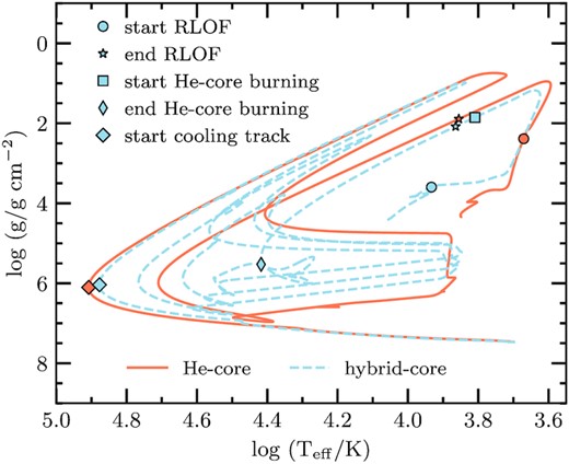
The Kiel diagram showing the formation and the cooling evolution of a 0.338 M⊙ He- (solid orange line) and hybrid-core (dashed blue line) WD. The initial binary parameters are Mdonor = 1.3 M⊙, Maccretor =1.2 M⊙, Pinitial = ∼16.982 d for the He-core model, and Mdonor = 2.3 M⊙, Maccretor =2.0 M⊙, Pinitial = ∼1.990 d for the hybrid-core model, at an initial metallicity of Z= 0.01. In both cases, the accretor is treated as a point mass. The evolutionary tracks are computed from ZAMS until the effective temperature of the WD reaches 5 000 K. The symbols mark various stages of evolution. The beginning and the end of the mass-transfer phase are represented by the circle and star symbol, respectively, the beginning and the end of the core-He burning phase (in the case of the hybrid-core sequence) are depicted by the square and thin diamond symbol, respectively, and finally the diamond symbol represents the beginning of the cooling track, i.e. the point when the evolutionary track reaches its maximum effective temperature.
The He-core WDs are formed by stripping mass when the donor star is on its red giant branch. The binary system consists of a low-mass donor star with an initial mass of 1.3 M⊙, a main-sequence companion of 1.2 M⊙, and an initial orbital period of ∼11.75 and ∼16.98 d, for the progenitor of the 0.325 M⊙ and 0.338 M⊙, respectively. After the end of the mass-transfer phase, the remnant evolves through the so-called proto-WD phase, in which unstable H burning leads to the occurrence of at least one H flash.
The initial binary configuration leading to the formation of the hybrid-core WDs is a 2.3 M⊙ intermediate-mass donor star with a companion of 2.0 M⊙, and an orbital period of 1.43 and ∼1.99 d, or the progenitor of the 0.325 M⊙ and 0.338 M⊙, respectively. The mass-transfer phase initiates during the Hertzsprung gap. Unlike the case of the He-core WD sequence, here the mass transfer ceases due to the core-He ignition. Shortly after the mass transfer ended, the remnant starts the core-He burning phase, which lasts around 670 Myr. Once the CO core is formed, the proto-WD undergoes four H shell flashes before finally settling on the cooling track.
2.3 WD cooling track
The WD sequences discussed in the previous section are formed through a stable mass-transfer channel. While it is possible that the first mass-transfer phase which leads to the formation of J1152+0248 −V is stable, we cannot rule out completely a common-envelope evolution. Additionally, the short orbital period of J1152+0248 (2.4 h) suggests that the second mass-transfer phase leading to the formation of the most massive component is unstable and proceeds through a common-envelope evolution. This evolutionary phase could possibly also affect the lower-mass component. Either way, there is an uncertainty in the mass of the H envelope available at the beginning of the cooling track resulting from the evolutionary history prior to the observed stage of the system.
The mass of the H envelope is one of the main factors that influence the cooling evolution of a WD. In order to take this uncertainty into account, we also computed WD cooling sequences with H envelopes thinner than the ones obtained from the binary evolutionary models described above. These sequences were computed using relaxation methods available in mesa. The initial conditions are taken at the point when the remnant reaches the beginning of the cooling track. Using the stellar profile at this point, we remove the desired amount of H, keeping the total mass unchanged (see Istrate et al., in preparation, for details).
Figs 3 and 4 show the WD radius as a function of the effective temperature for sequences with He- (top panels) and hybrid-core (bottom panels) and stellar mass of 0.338 M⊙ and 0.325 M⊙, respectively.
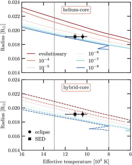
Stellar radius as a function of the effective temperature for both hybrid- (dashed lines) and He-core (solid lines) WD sequences with stellar mass 0.338 M⊙. The symbols correspond to the determinations of the effective temperature from observations (see Table 1). The dotted vertical lines indicate the blue and red edges of the observed instability strip for low-mass WDs (see Fig. 1).
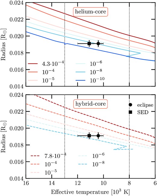
Same as Fig. 3 but for the WD sequences with stellar mass 0.325 M⊙.
For each core composition we consider different values of the H-envelope mass, starting from the value resulting from the binary evolution down to 10−8 M⊙. In particular, for the stellar mass of 0.325 M⊙ and He core, we also include a sequence with H-envelope mass of 10−10 M⊙. Overplotted are the measured values of J1152+0248 −V, both from the eclipse and the SED fitting.
As expected, the radius for the hybrid-core sequences is smaller than for the He-core sequences, for the same H-envelope mass. Intriguingly, the observations are not compatible with a thick H envelope, i.e. which obtained from binary evolution computations. For sequences characterized with a stellar mass of 0.338 M⊙ (see Fig. 3) the H-envelope mass consistent with the radius and effective temperature from Parsons et al. (2020) is between 10−4 and 10−6 M⊙ if we consider a hybrid core. For the sequences with an He core, the H-envelope mass is below 10−5 M⊙. For sequences with stellar mass of 0.325 M⊙ (see Fig. 4), the H-envelope mass needs to be even smaller to fit the observations, between 10−5 and 10−8 M⊙ for sequences with a hybrid core and between 10−5 and 10−10 M⊙ for sequences with an He core. Thus, J1152+0248 −V has an H envelope thinner than that obtained from evolutionary sequences, independently of the central chemical composition.
3 ADIABATIC PULSATIONS
In the case of WDs, the inner chemical structure is far from homogeneous, showing composition gradients (Althaus et al. 2010b). In this case, the asymptotic period spacing corresponds to the period spacing at the limit of very large values of k (Tassoul et al. 1990).
3.1 Numerical computations
For our pulsational computations we employed GYRE (Townsend & Teitler 2013; Townsend, Goldstein & Zweibel 2018), an open-source stellar oscillation code in its adiabatic form, version 5.0. Although GYRE is integrated within MESA, it was used as a stand-alone package. We performed a scan using a linear grid over a period range of 80−2000 s with alpha_osc = 100 and alpha_exp and alpha_ctr set to 50. The boundary conditions and variables were set to UNNO and DZIEM, respectively.1
We compute pulsations for He- and hybrid-core models in the effective temperature range of |$13\, 000$| and |$8\, 000$| K, which covers the empirical instability strip. We compute the period spectrum for ℓ = 1 and ℓ = 2 gravity modes with periods in a range of |$80 \ {\rm s} \le \Pi \le 2\, 000$| s.
3.2 Internal composition and the characteristic frequencies
To compare the pulsation properties of He- and hybrid-core WD models, we chose one template model for each central composition, with stellar mass of 0.338 M⊙, effective temperature of |$10\, 000$| K, and H-envelope mass of 10−4 M⊙. In the top panel of Figs 5 and 6, we depict the chemical profiles for an He- and a hybrid-core template models, respectively. Both template models show a pure H envelope, since gravitational settling had enough time to separate the elements in the outer layers. For the hybrid-core model we have a second chemical transition (He/C/O transition) around r/R ∼ 0.4, where the He abundance decreases towards the centre while the C and O abundance increase.
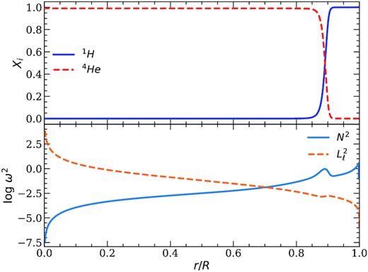
Internal profiles and characteristic frequencies for an He-core cooling sequence with M=0.338 M⊙, T|$_{\rm eff} = 10\, 000$| K, and MH = 10−4 M⊙. Top panel: The mass fraction of H and He as a function of the relative radius. Bottom panel: The logarithm of the Brunt-Väisälä (full blue line) and the Lamb (dashed orange line) characteristic frequencies as a function of the relative radius.
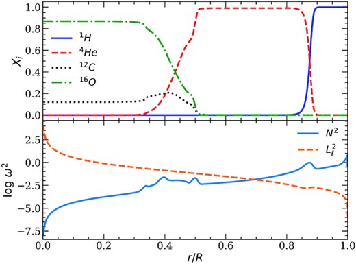
Internal chemical composition and characteristic frequencies for a hybrid-core sequence with M=0.338 M⊙, T|$_{\rm eff} = 10\, 000$| K, and MH = 10−4 M⊙. Top panel: Mass fraction of H, He, C, and O as a function of the relative radius. Bottom panel: The logarithm of the Brunt-Väisälä (full blue line) and Lamb (dashed orange line) characteristic frequencies as a function of the relative radius.
The presence of chemical transitions, where the abundances of nuclear species vary considerably in radius, modifies the conditions of the resonant cavity in which modes should propagate as standing waves. Specifically, the chemical transitions act as reflecting walls, trapping certain modes in a particular region of the star, where they show larger oscillation amplitudes. Trapped modes are those for which the wavelength of their radial eigenfunction matches the spatial separation between two chemical transitions or between a transition and the stellar centre or surface (Brassard et al. 1992b; Bradley, Winget & Wood 1993; Córsico et al. 2002).
The bottom panels of Figs 5 and 6 show the run of the logarithm of the Brunt-Väisälä and Lamb frequencies as a function of radius for the template models. The overall behaviour of log N2 is a general decrease with increasing stellar depth, eventually reaching small values in the deep core, as a consequence of degeneracy. As expected, the bumps in log N2 correspond to the chemical transition, where the chemical gradients have non-negligible values (Tassoul et al. 1990). For the He-core template model, the Brunt-Väisälä frequency shows only one bump corresponding to the H/He transition at r/R ∼ 0.9. For the hybrid-core template model, in addition to the bump at the base of the H envelope, the Brunt-Väisälä frequency shows a structure corresponding to the He/C/O transition around r/R ∼ 0.4. This transition is wide and shows three peaks due to the structure of the chemical gradients. We expect that the different profiles for the Brunt-Väisälä frequency for He-core and hybrid-core models will impact the pulsation properties, for example the period spectrum and the period spacing.
The Lamb frequency is only sensitive to the H/He transition at the bottom of the H envelope, as it is the case for ZZ Ceti stars (Romero et al. 2012). Thus, we do not believe the pressure modes could give information on the inner regions, if ever detected in low-mass WD stars.
4 RESULTS
4.1 Pulsational properties
As previously mentioned, for a chemically homogeneous and radiative star, the forward period spacing (ΔΠk = Πk + 1 − Πk) would be constant and given by the asymptotic period spacing, defined in equation (6). However, in the stratified inner structures, as the ones found in low-mass WDs, the forward period spacing deviates from a constant value, particularly for low-radial order modes. In this section, we will focus on models with stellar mass 0.338 M⊙. Similar results are found for models with stellar mass of 0.325 M⊙.
Fig. 7 shows the forward period spacing as a function of the period for ℓ = 1 modes. Top panels correspond to models with He core while bottom panels show the results for hybrid-core models. Finally, each column corresponds to sequences with different values for the H-envelope mass and each curve shows the forward period spacing at a different effective temperature along the cooling curve, from |$12\, 000$| K to 9000 K.
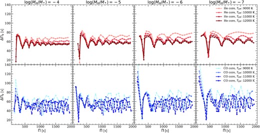
The forward period spacing (ΔΠk = Πk + 1 − Πk) as a function of the period for modes with ℓ = 1 for He- (top panels) and hybrid-core (bottom panels) models, with stellar mass 0.338 M⊙. Each column corresponds to a different H-envelope mass. In each plot, we show the period spacing for four effective temperatures along the cooling sequence, |$12\, 000$|, |$11\, 000$|, |$10\, 000$|, and 9000 K.
For the He-core models the distribution for the forward period spacing as a function of the period, shows a simple trapping cycle characteristic of one-transition models (Brassard et al. 1992b; Córsico & Althaus 2014), with defined local minima, as shown in the top panels of Fig. 7. For the hybrid-core models (bottom panels in Fig. 7) the pattern in the forward period spacing is more complex largely due to the influence of the He/C/O transition in the Brunt-Vaisälä frequency. Even though we expect the H/He transition to be dominant in the mode selection process, the presence of the second, broader, transition is not negligible. The differences in the pattern of the forward period spacing can be used to determine the inner composition of low-mass WDs, if enough consecutive periods are detected.
The trapping period, i.e. the period difference between two consecutive minima in ΔΠk, is longer for lower effective temperatures and thinner H envelopes. This effect is much more evident for the He-core models than for the hybrid-core models.
In general, we expect the forward period spacing to increase with decreasing effective temperature and thinner envelopes (Brassard et al. 1992b). This can be better explained in terms of the asymptotic period spacing, given by equation (6). The higher values for ΔΠa, and |$\overline{\Delta \Pi }$|, for lower effective temperatures result from the dependence of the Brunt-Väisälä frequency as |$N\propto \sqrt{\chi _{T}}$|, with χT → 0 for increasing degeneracy (T → 0) (see for instance Romero et al. 2012). In addition, the asymptotic period spacing, and the mean period spacing, are longer for thinner H envelopes (Tassoul et al. 1990).
If the stellar mass is fixed, the asymptotic period spacing for the He-core model is longer than that for the hybrid-core model, for the same effective temperature and H-envelope mass. This is related to the dependence of the Brunt-Väisälä frequency on the surface gravity N∝ g, where g ∝ M/R2. In this case, the radius is smaller for the hybrid-core models which leads to a larger value of the surface gravity (see Figs 3 and 4).
Finally, given the different chemical structure of He- and hybrid-core WD models, we expect different values for the period spectra as well. Fig. 8 shows the period difference between He- and the hybrid-core models, Πhe − Πhy as a function of the radial order k, for harmonic degree ℓ = 1. Each column corresponds to a different H-envelope mass, while the curves in each panel correspond to four different effective temperatures along the 0.338 M⊙ WD cooling track. In all cases, the difference in the periods between the He- and hybrid-core models are between ∼50 s, for k ≲ 10 and short periods, and ∼200 s for k ≳ 30 and longer periods. Note that the period difference is always positive, meaning that, for a given radial order, the period for the He-core model is larger than the one corresponding to the hybrid-core model. This is expected, since the periods, and the period spacing, vary as the inverse of the Brunt-Väisälä frequency, and thus the surface gravity (equation 7). As the period also increases with the cooling age, the period difference is larger for lower effective temperatures, particularly for modes with radial order k > 20. For future reference, we list the periods for ℓ = 1 and ℓ = 2, corresponding to the models considered in Fig. 8 and in Tables A1–A4.
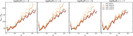
Period difference (Πhe − Πhy) as a function of the radial order for ℓ = 1 modes. The stellar mass is fixed to 0.338 M⊙. Each plot corresponds to a different H-envelope mass. We consider four effective temperatures.
4.2 Asteroseismology of J1152+0248 −V
For J1152+0248 −V Parsons et al. (2020) detected three pulsation periods, with the period of ∼1314 s being the one showing the highest amplitude. The list of observed periods and their corresponding amplitudes are listed in Table 2.
Observed pulsation periods and the corresponding amplitudes for J1152+0248 −V (Parsons et al. 2020).
| Period (s) | Amplitude (ppt) |
|---|---|
| 1314 ± 5.9 | 33.0 ± 1.3 |
| 1069 ± 13 | 9.8 ± 1.3 |
| 582.9 ± 4.3 | 8.9 ± 1.3 |
| Period (s) | Amplitude (ppt) |
|---|---|
| 1314 ± 5.9 | 33.0 ± 1.3 |
| 1069 ± 13 | 9.8 ± 1.3 |
| 582.9 ± 4.3 | 8.9 ± 1.3 |
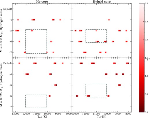
The value of χ2 (colour scale) as a function of the effective temperature and the mass of the H envelope. Top panels correspond to models with stellar mass 0.338 M⊙, while bottom panels show the results for 0.325 M⊙ models. Both He- (left-hand panels) and hybrid-core (right-hand panels) structures are considered. The dashed-line rectangle indicates the region of the Teff–H envelope plane restricted by the determinations of radius and effective temperature from Parsons et al. (2020).
If we combine our seismological results with the restrictions from the radius and the effective temperature presented in Parsons et al. (2020) (dashed-line rectangle in Fig. 9), the number of possible seismological solutions is largely reduced. In particular, the models characterized by a hybrid-core structure are the ones satisfying both criteria.
The best-fitting models for J1152+0248 −V are listed in Table 3. These models fit the observed periods within the uncertainties and are in agreement with the determinations of radius and effective temperature presented by Parsons et al. (2020). Note that all the models are characterized by an H-envelope mass of 10−6 M⊙ and a hybrid core. Thus, we can conclude that J1152+0248 −V is a low-mass WD star with a hybrid core and a thin H envelope.
Asteroseismological models for the low-mass WD J1152+0248 −V. The effective temperature, H-envelope mass, and central composition are listed in columns 2, 3, and 4, respectively. We list the theoretical periods that better fit the observed periods in column 4, along with the values of ℓ and k, in columns 6 and 7. The value of the quality function χ2 is listed in column 8.
| # | Teff (K) | R/R⊙ | M*/M⊙ | MH/M⊙ | XC | Πth (s) | ℓ | k | χ2 (s) |
|---|---|---|---|---|---|---|---|---|---|
| 1 | |$10\,917$| | 0.0187 | 0.338 | 10−6 | C/O | 1315.4 | 1 | 21 | 0.296 |
| 1063.3 | 2 | 30 | – | ||||||
| 582.01 | 2 | 15 | – | ||||||
| 2 | |$10\, 904$| | 0.0187 | 0.338 | 10−6 | C/O | 1316.1 | 1 | 21 | 0.305 |
| 1063.8 | 2 | 30 | – | ||||||
| 582.3 | 2 | 15 | – | ||||||
| 3 | |$10\, 929$| | 0.0187 | 0.338 | 10−6 | C/O | 1314.9 | 1 | 21 | 0.318 |
| 1062.8 | 2 | 30 | – | ||||||
| 581.8 | 2 | 15 | – | ||||||
| 4 | |$11\, 717$| | 0.0195 | 0.325 | 10−6 | C/O | 1316.1 | 1 | 21 | 0.345 |
| 1066.4 | 2 | 30 | – | ||||||
| 581.3 | 2 | 15 | – |
5 CONCLUSIONS
In this work, we explore the inner chemical structure of the pulsating low-mass WD in the J1152+0248 system using asteroseismology as a tool. This is the first pulsating low-mass WD in an eclipsing binary system with another low-mass WD which allows constraining the mass and radius of each component independently of evolutionary models.
We use low-mass WDs models with a stellar mass of 0.325 and 0.338 M⊙ and an He core and hybrid core, respectively, resulting from fully binary evolutionary computations. In addition, to account for the uncertainty in the H-envelope mass due to the evolution through a common-envelope channel, we use WD sequences with the same stellar mass but with an H envelope thinner than the canonical value obtained from stable mass transfer, i.e. from 10−4 to 10−10 M⊙. For all these sequences, we calculate adiabatic pulsations for effective temperatures in the range |$13\, 000$| K ≤Teff ≤ 8000 K.
We perform a study on the pulsating low-mass WD in the binary system J1152+0248 to uncover its inner chemical composition. By comparing the determinations of the radius and effective temperature presented by Parsons et al. (2020) with theoretical models (Istrate et al., in preparation), we find that the variable component of J1152+0248 must have an H envelope thinner than that predicted from stable mass-transfer binary evolution computations.
From the asteroseismological study we find a best-fitting model characterized by M* = 0.338 M⊙, |$T_{\rm eff}=10\,917$| K, MH/M⊙ = 10−6, and a hybrid-core composition. In particular, all local minima of χ2 correspond to models with hybrid core and a thin H envelope.
A systematic study of the pulsational properties and the observed period spectrum of low-mas WDs can give valuable information on the inner structure of these objects. This will help in disentangling the two WD populations coexisting in the mass interval ∼0.32–0.45 M⊙ which in turn leads to clues of the underlying progenitor population.
ACKNOWLEDGEMENTS
ADR and GRL acknowledge the support of the Coordenação de Aperfeiçoamento de Pessoal de Nível Superior – Brazil (CAPES) – Finance Code 001, and by Conselho Nacional de Desenvolvimento Científico e Tecnológico - Brazil (CNPq). AGI acknowledges support from the Netherlands Organisation for Scientific Research (NWO). SGP acknowledges the support of a Science and Technology Facilities Council (STFC) Ernest Rutherford Fellowship. Special thanks to Pablo Marchant, Josiah Schwab, and Jocelyn Goldstein for their help with numerical debugging and to the developers of MESA and GYRE for their continuous efforts to improve and extend these codes. This research has made use of NASA’s Astrophysics Data System and open source software such as the Python 3 language (Python Core Team 2015), the ipython kernel (Pérez & Granger 2007), the Jupyter Project (Kluyver et al. 2016), and the packages matplotlib (Hunter 2007), pandas (McKinney 2010), and the scipy ecosystem (Virtanen et al. 2019).
DATA AVAILABILITY
As an effort to promote open science, the results and codes to reproduce our results are available at https://zenodo.org/communities/mesa/.
Footnotes
The inlist and all its configuration settings can be found in here (link to be updated).
REFERENCES
APPENDIX A: THEORETICAL PERIODS
Period values for ℓ = 1 and ℓ = 2 modes corresponding to models with M* = 0.338 M⊙, effective temperature of |$12\, 000$| K, and H-envelope mass of 10−4, 10−5, and 10−6 M⊙.
| MH/M⊙ | 10−4 | 10−5 | 10−6 | ||||
|---|---|---|---|---|---|---|---|
| ℓ | k | He | C/O | He | C/O | He | C/O |
| 1 | 1 | 204.948 | 146.886 | 218.643 | 147.610 | 220.319 | 148.418 |
| 1 | 2 | 221.260 | 192.002 | 273.896 | 239.660 | 291.871 | 252.223 |
| 1 | 3 | 292.114 | 252.597 | 296.524 | 255.774 | 356.006 | 305.175 |
| 1 | 4 | 364.331 | 322.131 | 369.816 | 326.066 | 376.420 | 328.547 |
| 1 | 5 | 420.666 | 362.298 | 442.175 | 391.085 | 442.595 | 392.939 |
| 1 | 6 | 465.821 | 405.630 | 507.842 | 447.835 | 512.597 | 468.370 |
| 1 | 7 | 518.050 | 469.162 | 560.626 | 494.718 | 583.536 | 541.930 |
| 1 | 8 | 578.586 | 529.785 | 606.713 | 557.217 | 650.957 | 592.739 |
| 1 | 9 | 636.102 | 573.359 | 665.303 | 607.547 | 704.944 | 632.512 |
| 1 | 10 | 682.723 | 620.481 | 727.082 | 659.543 | 752.211 | 684.640 |
| 1 | 11 | 739.842 | 677.741 | 786.677 | 710.230 | 810.293 | 739.861 |
| 1 | 12 | 798.462 | 723.525 | 838.796 | 749.740 | 873.722 | 778.522 |
| 1 | 13 | 849.341 | 756.759 | 892.586 | 794.649 | 937.811 | 838.306 |
| 1 | 14 | 902.294 | 808.744 | 954.758 | 856.940 | 997.247 | 898.565 |
| 1 | 15 | 960.397 | 864.535 | 1014.63 | 912.796 | 1051.18 | 952.676 |
| 1 | 16 | 1014.40 | 919.221 | 1067.36 | 959.175 | 1106.24 | 991.396 |
| 1 | 17 | 1066.15 | 959.235 | 1122.26 | 1002.96 | 1168.11 | 1052.52 |
| 1 | 18 | 1122.16 | 1004.73 | 1182.63 | 1062.39 | 1231.03 | 1116.87 |
| 1 | 19 | 1177.61 | 1061.12 | 1240.57 | 1121.12 | 1289.88 | 1166.22 |
| 1 | 20 | 1229.32 | 1121.06 | 1294.31 | 1165.97 | 1343.50 | 1203.20 |
| 2 | 1 | 120.014 | 100.316 | 141.344 | 100.940 | 142.736 | 101.493 |
| 2 | 2 | 142.587 | 111.277 | 160.508 | 139.347 | 185.489 | 150.999 |
| 2 | 3 | 185.975 | 151.547 | 187.659 | 152.494 | 209.625 | 176.847 |
| 2 | 4 | 225.657 | 191.494 | 231.584 | 194.754 | 232.453 | 195.717 |
| 2 | 5 | 254.034 | 211.840 | 272.358 | 229.803 | 273.019 | 231.131 |
| 2 | 6 | 281.506 | 237.353 | 307.956 | 260.380 | 314.097 | 273.528 |
| 2 | 7 | 314.200 | 273.648 | 334.955 | 288.159 | 354.935 | 316.423 |
| 2 | 8 | 349.925 | 308.696 | 364.899 | 326.241 | 319.257 | 347.570 |
| 2 | 9 | 379.496 | 336.314 | 400.421 | 358.342 | 418.988 | 372.001 |
| 2 | 10 | 408.479 | 365.660 | 435.919 | 386.702 | 449.058 | 401.706 |
| 2 | 11 | 443.206 | 396.338 | 468.693 | 416.106 | 484.623 | 439.694 |
| 2 | 12 | 475.033 | 425.943 | 497.913 | 452.092 | 521.580 | 476.215 |
| 2 | 13 | 504.023 | 461.149 | 531.857 | 483.738 | 557.625 | 498.294 |
| 2 | 14 | 536.607 | 486.195 | 567.956 | 503.483 | 590.826 | 524.268 |
| 2 | 15 | 569.643 | 506.188 | 600.466 | 533.089 | 621.325 | 560.439 |
| 2 | 16 | 599.506 | 538.593 | 630.662 | 570.281 | 655.268 | 596.169 |
| 2 | 17 | 630.599 | 572.313 | 664.302 | 597.936 | 691.754 | 617.974 |
| 2 | 18 | 663.345 | 594.209 | 699.097 | 619.426 | 727.368 | 649.520 |
| 2 | 19 | 694.175 | 617.784 | 731.092 | 652.467 | 759.583 | 684.916 |
| 2 | 20 | 724.441 | 652.464 | 762.392 | 689.291 | 791.026 | 716.668 |
| 2 | 21 | 756.787 | 684.847 | 795.637 | 714.925 | 825.950 | 738.317 |
| 2 | 22 | 787.930 | 709.047 | 829.417 | 737.077 | 861.764 | 774.935 |
| 2 | 23 | 818.226 | 731.327 | 861.601 | 772.178 | 895.634 | 813.010 |
| 2 | 24 | 849.940 | 764.288 | 893.184 | 810.806 | 927.753 | 848.125 |
| 2 | 25 | 881.227 | 800.000 | 926.496 | 843.600 | 960.895 | 870.022 |
| 2 | 26 | 911.804 | 833.115 | 959.922 | 863.817 | 995.764 | 902.046 |
| 2 | 27 | 943.122 | 853.700 | 991.721 | 894.125 | 1030.54 | 939.114 |
| 2 | 28 | 974.435 | 879.080 | 1023.75 | 930.100 | 1063.74 | 966.625 |
| 2 | 29 | 1005.23 | 913.682 | 1057.21 | 956.318 | 1096.41 | 989.506 |
| 2 | 30 | 1036.10 | 941.506 | 1089.98 | 978.538 | 1130.42 | 1026.26 |
Period values for ℓ = 1 and ℓ = 2 modes corresponding to models with M* = 0.338 M⊙, effective temperature of |$11\, 000$| K, and H-envelope mass of 10−4, 10−5, and 10−6 M⊙.
| MH/M⊙ | 10−4 | 10−5 | 10−6 | ||||
|---|---|---|---|---|---|---|---|
| ℓ | k | He | C/O | He | C/O | He | C/O |
| 1 | 1 | 207.777 | 151.919 | 233.957 | 152.645 | 235.524 | 153.322 |
| 1 | 2 | 234.935 | 193.714 | 276.833 | 243.947 | 307.762 | 266.071 |
| 1 | 3 | 308.929 | 266.516 | 311.893 | 268.497 | 361.733 | 309.919 |
| 1 | 4 | 380.793 | 335.386 | 389.048 | 342.310 | 391.382 | 343.863 |
| 1 | 5 | 433.845 | 372.487 | 463.274 | 408.527 | 463.749 | 411.409 |
| 1 | 6 | 481.618 | 420.763 | 528.221 | 461.074 | 537.098 | 489.063 |
| 1 | 7 | 538.336 | 486.755 | 577.219 | 513.621 | 610.573 | 564.377 |
| 1 | 8 | 602.632 | 547.503 | 629.465 | 582.118 | 676.213 | 616.106 |
| 1 | 9 | 655.766 | 598.093 | 692.730 | 635.549 | 725.608 | 655.982 |
| 1 | 10 | 707.296 | 647.314 | 756.426 | 681.750 | 779.270 | 707.562 |
| 1 | 11 | 769.074 | 697.705 | 814.497 | 731.479 | 843.416 | 768.330 |
| 1 | 12 | 825.765 | 746.133 | 866.850 | 782.429 | 909.524 | 813.564 |
| 1 | 13 | 877.491 | 789.346 | 928.721 | 827.532 | 973.853 | 868.318 |
| 1 | 14 | 936.544 | 836.128 | 992.887 | 884.697 | 1032.09 | 927.724 |
| 1 | 15 | 994.745 | 890.138 | 1049.75 | 944.978 | 1087.01 | 992.624 |
| 1 | 16 | 1047.83 | 952.948 | 1104.48 | 1003.92 | 1149.66 | 1032.11 |
| 1 | 17 | 1104.56 | 1002.48 | 1166.22 | 1038.52 | 1215.34 | 1085.88 |
| 1 | 18 | 1162.76 | 1035.48 | 1227.62 | 1092.55 | 1277.54 | 1149.55 |
| 1 | 19 | 1216.77 | 1091.03 | 1283.50 | 1156.59 | 1333.40 | 1211.86 |
| 1 | 20 | 1272.22 | 1153.26 | 1340.63 | 1216.10 | 1392.04 | 1256.28 |
| 2 | 1 | 120.711 | 103.726 | 149.787 | 104.375 | 151.814 | 104.829 |
| 2 | 2 | 151.834 | 112.262 | 162.269 | 141.279 | 194.448 | 158.655 |
| 2 | 3 | 195.703 | 159.298 | 197.606 | 160.112 | 211.759 | 179.466 |
| 2 | 4 | 234.191 | 198.316 | 243.168 | 203.875 | 243.337 | 204.548 |
| 2 | 5 | 261.843 | 218.039 | 284.536 | 239.630 | 285.963 | 241.754 |
| 2 | 6 | 291.547 | 246.112 | 318.537 | 267.939 | 328.974 | 285.360 |
| 2 | 7 | 327.190 | 283.652 | 345.423 | 299.045 | 370.474 | 328.794 |
| 2 | 8 | 362.990 | 318.254 | 379.569 | 339.961 | 404.184 | 360.358 |
| 2 | 9 | 390.988 | 350.257 | 416.755 | 375.420 | 431.958 | 388.493 |
| 2 | 10 | 424.473 | 383.250 | 452.823 | 402.049 | 466.541 | 417.648 |
| 2 | 11 | 459.804 | 409.554 | 483.925 | 429.733 | 504.598 | 454.562 |
| 2 | 12 | 490.304 | 438.938 | 516.320 | 467.240 | 542.571 | 490.865 |
| 2 | 13 | 521.968 | 475.075 | 553.706 | 498.686 | 578.574 | 513.862 |
| 2 | 14 | 556.885 | 500.928 | 589.250 | 519.210 | 610.434 | 540.633 |
| 2 | 15 | 588.750 | 521.371 | 620.508 | 550.428 | 644.063 | 580.230 |
| 2 | 16 | 620.001 | 555.159 | 654.070 | 590.481 | 681.677 | 621.644 |
| 2 | 17 | 653.702 | 590.195 | 690.425 | 625.170 | 719.126 | 649.981 |
| 2 | 18 | 686.347 | 622.643 | 724.303 | 648.467 | 753.175 | 671.000 |
| 2 | 19 | 717.267 | 644.476 | 756.359 | 674.238 | 785.390 | 707.347 |
| 2 | 20 | 750.538 | 671.115 | 790.585 | 711.447 | 821.198 | 745.512 |
| 2 | 21 | 783.051 | 704.597 | 825.706 | 743.906 | 858.469 | 768.119 |
| 2 | 22 | 814.218 | 737.499 | 859.058 | 764.570 | 893.692 | 799.575 |
| 2 | 23 | 846.959 | 757.240 | 891.796 | 797.047 | 926.893 | 838.324 |
| 2 | 24 | 879.365 | 785.944 | 926.331 | 835.814 | 961.390 | 878.146 |
| 2 | 25 | 911.008 | 822.649 | 960.885 | 872.099 | 997.639 | 907.292 |
| 2 | 26 | 943.351 | 858.165 | 993.755 | 900.244 | 1033.59 | 933.155 |
| 2 | 27 | 975.716 | 887.886 | 1027.15 | 924.922 | 1067.91 | 970.154 |
| 2 | 28 | 1007.49 | 908.910 | 1061.95 | 960.303 | 1101.84 | 1008.85 |
| 2 | 29 | 1072.09 | 940.675 | 1095.65 | 997.176 | 1137.52 | 1034.44 |
| 2 | 30 | 1103.79 | 975.775 | 1128.77 | 1024.26 | 1173.68 | 1060.13 |
Period values for ℓ = 1 and ℓ = 2 modes corresponding to models with M* = 0.338 M⊙, effective temperature of |$10\, 000$| K, and H-envelope mass of 10−4, 10−5, and 10−6 M⊙.
| MH/M⊙ | 10−4 | 10−5 | 10−6 | ||||
|---|---|---|---|---|---|---|---|
| ℓ | k | He | C/O | He | C/O | He | C/O |
| 1 | 1 | 209.850 | 157.321 | 252.328 | 157.951 | 254.801 | 158.549 |
| 1 | 2 | 253.518 | 195.924 | 280.175 | 248.189 | 326.917 | 283.059 |
| 1 | 3 | 329.045 | 283.798 | 331.577 | 285.471 | 366.984 | 315.927 |
| 1 | 4 | 398.872 | 349.747 | 411.843 | 361.596 | 412.719 | 362.727 |
| 1 | 5 | 449.743 | 386.155 | 487.861 | 248.295 | 490.081 | 433.524 |
| 1 | 6 | 501.311 | 439.089 | 550.052 | 476.945 | 567.284 | 513.238 |
| 1 | 7 | 564.292 | 507.595 | 598.176 | 536.112 | 642.441 | 588.261 |
| 1 | 8 | 629.238 | 566.539 | 658.379 | 608.287 | 703.193 | 639.718 |
| 1 | 9 | 679.188 | 625.059 | 725.480 | 662.554 | 752.760 | 680.114 |
| 1 | 10 | 739.471 | 673.875 | 790.184 | 704.021 | 815.755 | 733.170 |
| 1 | 11 | 802.594 | 718.873 | 845.394 | 756.443 | 884.549 | 800.999 |
| 1 | 12 | 856.823 | 772.083 | 904.980 | 819.879 | 953.196 | 856.930 |
| 1 | 13 | 914.781 | 828.101 | 972.970 | 868.674 | 1017.90 | 905.083 |
| 1 | 14 | 977.584 | 871.154 | 1036.10 | 918.761 | 1075.56 | 964.206 |
| 1 | 15 | 1034.07 | 923.283 | 1092.89 | 982.771 | 1138.42 | 1034.76 |
| 1 | 16 | 1091.60 | 988.449 | 1155.57 | 1045.98 | 1208.10 | 1074.30 |
| 1 | 17 | 1153.16 | 1042.38 | 1222.19 | 1076.96 | 1277.21 | 1124.88 |
| 1 | 18 | 1211.49 | 1072.43 | 1284.28 | 1129.61 | 1341.23 | 1190.77 |
| 1 | 19 | 1268.95 | 1127.11 | 1344.28 | 1199.66 | 1402.32 | 1264.19 |
| 1 | 20 | 1330.48 | 1189.77 | 1408.16 | 1267.85 | 1468.56 | 1325.45 |
| 2 | 1 | 121.586 | 107.287 | 157.518 | 107.919 | 163.156 | 108.312 |
| 2 | 2 | 163.416 | 113.564 | 167.306 | 143.524 | 203.910 | 168.026 |
| 2 | 3 | 206.981 | 168.965 | 209.618 | 169.896 | 216.181 | 183.062 |
| 2 | 4 | 243.544 | 205.790 | 256.828 | 214.873 | 257.004 | 215.468 |
| 2 | 5 | 271.659 | 226.439 | 298.421 | 250.869 | 302.091 | 254.650 |
| 2 | 6 | 304.270 | 256.870 | 329.841 | 277.285 | 347.023 | 299.360 |
| 2 | 7 | 343.101 | 295.672 | 359.639 | 312.151 | 388.134 | 342.354 |
| 2 | 8 | 376.609 | 329.099 | 397.374 | 355.056 | 418.378 | 374.155 |
| 2 | 9 | 406.703 | 365.975 | 436.177 | 392.490 | 450.250 | 406.368 |
| 2 | 10 | 443.943 | 400.944 | 471.367 | 418.069 | 489.031 | 434.251 |
| 2 | 11 | 478.181 | 424.514 | 502.886 | 445.030 | 529.062 | 470.434 |
| 2 | 12 | 509.339 | 453.685 | 540.512 | 483.040 | 568.103 | 506.993 |
| 2 | 13 | 545.056 | 489.279 | 579.302 | 514.825 | 603.410 | 532.999 |
| 2 | 14 | 580.024 | 516.482 | 613.501 | 538.859 | 637.183 | 562.265 |
| 2 | 15 | 612.022 | 540.797 | 647.314 | 572.300 | 675.967 | 604.029 |
| 2 | 16 | 646.904 | 574.901 | 685.322 | 612.391 | 716.491 | 646.414 |
| 2 | 17 | 981.976 | 609.741 | 722.939 | 649.241 | 755.304 | 682.219 |
| 2 | 18 | 714.771 | 647.571 | 757.683 | 684.100 | 790.917 | 702.311 |
| 2 | 19 | 749.324 | 679.309 | 793.296 | 703.049 | 827.350 | 735.388 |
| 2 | 20 | 784.642 | 696.728 | 831.114 | 737.108 | 866.985 | 777.381 |
| 2 | 21 | 818.136 | 728.585 | 868.816 | 774.163 | 907.360 | 807.014 |
| 2 | 22 | 852.723 | 764.778 | 904.819 | 802.704 | 946.459 | 832.156 |
| 2 | 23 | 888.137 | 792.796 | 941.137 | 828.950 | 984.102 | 871.453 |
| 2 | 24 | 922.537 | 815.698 | 979.211 | 866.280 | 1021.99 | 914.490 |
| 2 | 25 | 957.299 | 850.262 | 1017.29 | 905.561 | 1061.17 | 951.177 |
| 2 | 26 | 992.689 | 887.230 | 1053.93 | 942.024 | 1101.43 | 976.345 |
| 2 | 27 | 1027.87 | 923.354 | 1090.87 | 966.846 | 1141.57 | 1011.69 |
| 2 | 28 | 1062.61 | 950.145 | 1129.15 | 998.759 | 1180.46 | 1053.86 |
| 2 | 29 | 1098.14 | 975.476 | 1167.12 | 1038.43 | 1219.08 | 1088.51 |
| 2 | 30 | 1133.72 | 1011.07 | 1204.56 | 1074.88 | 1258.10 | 1110.10 |
Period values for ℓ = 1 and ℓ = 2 modes corresponding to models with M* = 0.338 M⊙, effective temperature of |$9\, 000$| K, and H-envelope mass of 10−4, 10−5, and 10−6 M⊙.
| MH/M⊙ | 10−4 | 10−5 | 10−6 | ||||
|---|---|---|---|---|---|---|---|
| ℓ | k | He | C/O | He | C/O | He | C/O |
| 1 | 1 | 211.971 | 163.184 | 272.688 | 163.728 | 278.506 | 164.253 |
| 1 | 2 | 276.632 | 198.670 | 286.577 | 253.161 | 349.212 | 303.724 |
| 1 | 3 | 352.387 | 305.461 | 355.981 | 307.717 | 375.098 | 324.564 |
| 1 | 4 | 418.508 | 365.398 | 439.196 | 385.267 | 440.661 | 386.324 |
| 1 | 5 | 469.126 | 404.819 | 516.118 | 451.060 | 523.307 | 460.588 |
| 1 | 6 | 526.313 | 461.883 | 573.907 | 497.554 | 604.686 | 542.008 |
| 1 | 7 | 595.997 | 532.423 | 627.193 | 563.328 | 680.545 | 615.165 |
| 1 | 8 | 657.552 | 589.357 | 695.003 | 637.210 | 738.264 | 665.314 |
| 1 | 9 | 711.747 | 653.526 | 766.831 | 686.424 | 797.295 | 704.490 |
| 1 | 10 | 780.216 | 697.500 | 833.735 | 731.373 | 868.130 | 768.783 |
| 1 | 11 | 843.534 | 745.433 | 893.015 | 793.537 | 942.846 | 847.662 |
| 1 | 12 | 901.897 | 808.247 | 961.966 | 869.583 | 1019.19 | 918.324 |
| 1 | 13 | 968.255 | 875.514 | 1036.37 | 928.897 | 1094.93 | 970.636 |
| 1 | 14 | 1035.46 | 925.732 | 1106.85 | 979.084 | 1164.70 | 1031.76 |
| 1 | 15 | 1097.32 | 977.308 | 1172.29 | 1045.33 | 1233.01 | 1100.78 |
| 1 | 16 | 1162.30 | 1043.90 | 1241.03 | 1107.19 | 1306.57 | 1139.70 |
| 1 | 17 | 1230.74 | 1099.27 | 1314.57 | 1145.56 | 1383.92 | 1213.45 |
| 1 | 18 | 1296.20 | 1132.24 | 1387.83 | 1214.51 | 1462.30 | 1297.58 |
| 1 | 19 | 1360.81 | 1197.61 | 1458.53 | 1291.93 | 1539.71 | 1374.64 |
| 1 | 20 | 1429.04 | 1270.06 | 1527.91 | 1369.63 | 1614.85 | 1424.85 |
| 2 | 1 | 122.673 | 111.022 | 161.731 | 111.709 | 177.473 | 112.048 |
| 2 | 2 | 177.534 | 115.239 | 179.106 | 146.305 | 211.221 | 178.889 |
| 2 | 3 | 219.601 | 181.074 | 224.211 | 182.664 | 226.761 | 188.896 |
| 2 | 4 | 254.109 | 214.244 | 273.063 | 228.523 | 274.394 | 229.265 |
| 2 | 5 | 283.806 | 237.817 | 313.728 | 263.906 | 322.327 | 270.651 |
| 2 | 6 | 320.563 | 270.466 | 343.764 | 289.721 | 369.126 | 316.276 |
| 2 | 7 | 361.292 | 310.114 | 378.605 | 328.255 | 408.989 | 358.240 |
| 2 | 8 | 392.415 | 342.644 | 419.762 | 372.913 | 440.332 | 391.682 |
| 2 | 9 | 428.280 | 384.076 | 460.811 | 410.346 | 478.305 | 423.698 |
| 2 | 10 | 467.738 | 417.823 | 496.879 | 433.479 | 507.736 | 451.141 |
| 2 | 11 | 502.082 | 439.454 | 532.901 | 463.571 | 564.517 | 493.970 |
| 2 | 12 | 537.746 | 471.766 | 575.233 | 507.100 | 608.865 | 537.519 |
| 2 | 13 | 577.290 | 510.640 | 617.606 | 544.610 | 651.321 | 570.193 |
| 2 | 14 | 614.507 | 543.309 | 656.751 | 574.361 | 690.583 | 602.753 |
| 2 | 15 | 650.556 | 573.042 | 694.888 | 610.217 | 731.419 | 647.504 |
| 2 | 16 | 689.501 | 608.268 | 736.295 | 655.098 | 775.176 | 697.196 |
| 2 | 17 | 728.692 | 646.436 | 779.002 | 698.230 | 820.347 | 733.340 |
| 2 | 18 | 765.618 | 688.715 | 820.721 | 730.570 | 865.547 | 756.089 |
| 2 | 19 | 804.125 | 724.033 | 861.022 | 752.829 | 909.721 | 799.923 |
| 2 | 20 | 843.683 | 741.825 | 901.474 | 797.069 | 952.601 | 844.521 |
| 2 | 21 | 882.106 | 778.876 | 943.447 | 839.523 | 995.140 | 871.128 |
| 2 | 22 | 920.408 | 820.648 | 986.213 | 865.190 | 1038.45 | 909.888 |
| 2 | 23 | 959.520 | 851.564 | 1028.20 | 898.880 | 1082.74 | 959.228 |
| 2 | 24 | 998.867 | 876.304 | 1069.13 | 645.024 | 1127.70 | 1003.20 |
| 2 | 25 | 1037.62 | 916.100 | 1110.60 | 988.842 | 1172.86 | 1032.01 |
| 2 | 26 | 1076.42 | 958.321 | 1153.10 | 1019.67 | 1217.46 | 1070.84 |
| 2 | 27 | 1116.01 | 995.860 | 1195.53 | 1052.01 | 1261.71 | 1117.93 |
| 2 | 28 | 1155.22 | 1022.68 | 1237.56 | 1095.90 | 1305.52 | 1157.13 |
| 2 | 29 | 1194.12 | 1057.21 | 1279.30 | 1137.63 | 1349.21 | 1187.67 |
| 2 | 30 | 1233.58 | 1097.80 | 1321.30 | 1166.17 | 1393.53 | 1231.34 |
