The GALAH Survey: dependence of elemental abundances on age and metallicity for stars in the Galactic disc

ABSTRACT

1 INTRODUCTION

Understanding the formation and evolution of the Milky Way is a major challenge for modern astronomy. Importantly, stellar age and composition can reveal the key aspects of the evolution in this regard. The usefulness of the chemical composition stems from three key facts (Pagel 2009). First, except for a few elements like H, He, Li, and B that are made by the big bang nucelosynthesis, all elements are synthesized in the interiors of stars and are released into the surrounding gas thereby enriching it when stars die. Successive generation of stars are born out of gas enriched by previous generations, which means chemical information is passed down from one generation of stars to the next. Secondly, although stars synthesize new elements in their interior, their surface composition remains, with some exceptions, largely unchanged and this is what we observe and measure. Hence, the surface chemical composition of stars encode the information about the environment from which they were born (Freeman & Bland-Hawthorn 2002). Finally, there are various production sites for chemical elements (such as core collapse supernovae (SN), explosion of white dwarfs in binary systems, and asymptotic giant branch stars) and the nucleosynthetic yields of elements varies from one site to another. The occurrence rate of the various sites change with time and location. This means that the information carried by the different elements is not the same but is rich and useful when considered as an ensemble.

There is a rich history of chemical evolution models trying to predict the distribution of age and elemental abundances for stars in the Galaxy, including analytical models, semi-analytical models, and cosmological simulations (Chiappini, Matteucci & Gratton 1997; Schönrich & Binney 2009; Minchev, Chiappini & Martig 2013; Kubryk, Prantzos & Athanassoula 2015; Andrews et al. 2017; Mackereth et al. 2018; Buck 2020; Kobayashi, Karakas & Lugaro 2020). However, understanding chemical enrichment of the Galaxy from first principles is challenging. Chemical enrichment is the outcome of multiple physical process occurring simultaneously over the lifetime of the Galaxy, and most of these processes are poorly understood. Some aspects of modelling the chemical evolution like the distribution of stellar masses and the fraction of stars dying at any given time are dictated by the initial mass function and the theory of stellar evolution, which are known relatively well (Krumholz 2014; Marigo et al. 2017). However, some of the other crucial aspects are not, including the star formation history, the radial distribution of gas, the infall of fresh gas, the outflow of enriched gas, the radial transport of enriched gas in the disc, and the nucleosynthetic yields of different elements.

The limitations of chemical evolution models have prompted the use of data-driven/empirical methods to disentangle the information hidden in the chemical abundances of Galactic stars. Examples of data-driven approaches that exclusively explore the elemental abundance space are Ting, Conroy & Goodman (2015) and Casey et al. (2019). While these are useful for understanding the role of different nucleosynthetic processes, they are less useful for understanding the evolution as they do not directly take the age or the location of stars into account.

Empirical studies of how elemental abundances depend on age have also been performed, providing useful insights into the chemical evolution in the Galaxy. Using a sample of 189 nearby dwarfs, Edvardsson et al. (1993) showed that for a given age and orbital radius (equivalent to metallicity because age and radius correlated for their sample), stars have a small dispersion (0.05 dex) in [α/Fe]. They suggested that this indicates that the products of nuclear synthesis from SNe are well mixed in the interstellar medium (hereafter ISM). The scatter in [X/Fe] for heavy elements like Ba, Y, Zr, and Nd, for a given age and metallicity, was also claimed to be compatible with measurement errors. Nissen (2015), using 21 solar twins with better measurement precision and more elements, reported a small scatter in elemental abundances for a given age (see also da Silva et al. 2012; Nissen et al. 2017). s-process element Y was also shown to have a tight correlation with age. Bedell et al. (2018) further expanded the analysis of solar twins using 79 stars and studying trends of 30 elements. They showed that stars having similar age and metallicity have nearly identical elemental abundances (see also Spina et al. 2016, 2018b). The high-precision analysis of age–abundance relations was extended to stars with a wide range in metallicities by several studies (Feltzing et al. (2017; Delgado Mena et al. 2019; Casali et al. 2020). They showed that a number of elements show abundance trends with age and much of the scatter for a given age can be attributed to metallicity. A few other studies exploring the age abundance relations include Lin et al. (2020), who explored trends with both age and metallicity using GALAH DR2, and Feuillet et al. (2018), who explored age trends of giants in the solar neighbourhood using APOGEE.

In a significant development, Ness et al. (2019) showed that abundances of 17 elements can be predicted from just age and metallicity, with intrinsic scatter about the predictions being only about 0.02 dex. Importantly, they showed that the abundance–age–metallicity relations are valid well beyond the solar Galactocentric radius. Unlike previous studies, which were based on dwarfs and main-sequence turn-off (MSTO) stars, they used red clump stars and hence they also verified that the abundance relations are not exclusive to dwarfs. However, Ness et al. (2019) only studied the low-α population, restricted to a narrow range in age and α abundances. They studied mainly α and iron peak elements, which are thought to be produced by SNe II and SNe Ia explosions. Elements produced by other mechanisms, for example, s-process elements from asymptotic giant branch (AGB) stars or r-process elements were not studied. Finally, in their study, age measurements that were independent of abundances were only available for stars in the solar Galactocentric radius.

The GALAH + survey, which has measured abundances of 30 elements for about 700 000 stars, has more than 50 000 MSTO stars and 4000 asteroseismic giants with reliable age and abundance measurements. This provides a new opportunity to study the dependence of elemental abundances on age and metallicity and to overcome the limitations of the previous studies, which is the aim of this paper. Using these data, we expand the study with significantly more stars than previous studies and to regions beyond the solar annulus. Compared to Ness et al. (2019), we also expand the analysis to include s- and r-process elements. Additionally, we compare and contrast the abundance trends for dwarfs with that for giants, whose ages are measured using independent techniques.

2 DATA

In this paper, we use data from the GALAH + DR3 catalogue (Buder et al. 2021), which, in addition to the main GALAH survey, also includes data from the TESS-HERMES (Sharma et al. 2018) and K2-HERMES (Sharma et al. 2019) surveys, which use the same spectrograph, observational setup, and data reduction pipeline as the GALAH survey. The catalogue provides spectroscopic stellar parameters T_eff, log g, and [Fe/H] and abundances for 30 elements. We focus on two specific type of stars, MSTO stars and asteroseismic red giants (RG) for which ages can reliably determined. The RG stars have asteroseismic information from the NASA K2 mission and their spectroscopic follow-up was carried out by the K2-HERMES survey.

The ages and distances for the MSTO and RG stars are computed with the bstep code (Sharma et al. 2018). bstep provides a Bayesian estimate of intrinsic stellar parameters from observed parameters by making use of stellar isochrones. For results presented in this paper, we use the PARSEC-COLIBRI stellar isochrones (Marigo et al. 2017). For the MSTO stars, we use the following observables: T_eff, log g, [Fe/H], [α/Fe], J, K_s, and parallax. For the RG stars, in addition to the above observables, we use the asteroseismic observables Δν and ν_max. These stars were observed as part of the K2 Galactic Archaeology Program (Stello et al. 2015) and include stars from campaigns 1 to 15 (Stello et al. 2017). The asteroseismic analysis is conducted with the method by Kallinger et al. (2010, 2014), known as the CAN pipeline. Δν and ν_max for the model stars along the isochrones are determined with the asfgrid code (Sharma et al. 2016) that incorporates corrections to the Δν scaling relation suggested by stellar models.

In order to test if the abundance–age–metallicity relations are local or valid over the Galaxy, it is important to sample different Galactocentric (R, z) locations. The distribution in the Galactocentric (R, z) plane of stars that we use in this paper is shown in Fig. 1. Also shown is the distribution in the (R_g, z) plane, where R_g = R(v_rot/232.0 km s⁻¹) is the guiding radius and v_rot is the azimuthal rotational velocity. The MSTO stars are intrinsically faint and hence are mainly confined within 1 kpc from the Sun. However, they do span a wide range in guiding radius, which makes it possible to study stars that were born beyond the solar neighbourhood. The RG stars span a wide range in both R and z and their R_g-span is also much larger.

Figure 1.

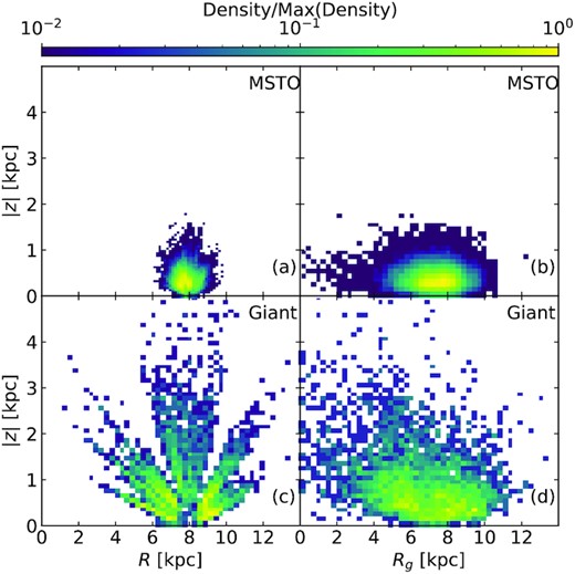
Distribution of MSTO (top panels) and giant stars (bottom panels) analysed in this paper shown in the (R, |z|) (left-hand panels) and (R_g, |z|) (right-hand panels) planes. The stars have signal-to-noise ratio (S/N) > 20.

Open in new tabDownload slide

3 RESULTS

3.1 Abundance trends with age and [Fe/H]

In Fig. 2, we show the median chemical abundances in the (age, [Fe/H]) plane for MSTO stars. The elements are ordered based on their gradient with respect to age and [Fe/H] (see Section 3.4 for more details).The abundances are shifted to be zero for solar age and metallicity, and are scaled with respect to the global spread (see the figure caption). A wide variety of trends can be seen. Some pronounced examples are as follows: (1) Elements Ba, Y, and Al show a gradient along the horizontal age axis, indicative of strong dependence on age and weak dependence on [Fe/H]. (2) Elements Cu, Mn, Cr, and Ni show a gradient along the vertical [Fe/H] axis, indicative of strong dependence on [Fe/H] and weak dependence on age. (3) Elements Mg, Si, Ca, Ti, O, and Sc show a diagonal gradient from the top left- to bottom right-hand side, indicative of strong dependence on both age and [Fe/H]. (4) Some have positive gradient with age (Ba and Y) while others have negative (Mg, Si). (5) Dependence of some elements is more complicated, for example, Na has a gradient with [Fe/H] that is positive for young stars and negative for older stars.

Figure 2.

Median abundance of different elements in the (age,[Fe/H]) plane for MSTO stars with S/N > 20. We standardize the median abundance in each bin by subtracting μ_X, the 50 percentile value, and then dividing by δ_X, the dispersion based on 16 and 84 percentile values. In each panel, the number of stars plotted is shown in the upper right-hand side and the δ_X is shown in the lower right-hand side. The elements are ordered based on their gradient with respect to age and [Fe/H]; see Section 3.4 for more details.

Open in new tabDownload slide

3.2 Scatter of abundances at fixed age and [Fe/H]

In Fig. 3, we show the abundance dispersion in the (age, [Fe/H]) plane for MSTO stars. The dispersion is shown relative to measurement uncertainty. The relative dispersion computed over all stars is labelled in each panel. All elements, except for Co, La, Li, and Zr, have relative dispersion that is small (less than 1.3). This suggests that the abundances can be predicted from age and metallicity. Very high dispersion for Co, Li, and Zr suggests there are other processes in addition to Galactic chemical evolution that play important roles in the chemical finger print we observe. For example, the abundance of Li is known to depend on surface gravity and temperature (Gao et al. 2020).

Figure 3.

Dispersion of elemental abundances in the (age,[Fe/H]) plane for MSTO stars with S/N > 20. The dispersion shown is around median values and is normalized by dividing with the uncertainty of each data point. The first panel shows the density of stars in (age,[Fe/H]) plane. In each panel, the number of stars plotted is shown in the upper right-hand side and the average dispersion relative to uncertainty for all stars is shown in the lower right-hand side.

Open in new tabDownload slide

For most elements, the dispersion is close to 1 over most regions of the (age, [Fe/H]) plane. However, some elements show slightly higher dispersion (dark brown regions) in certain specific regions. One reason for this could be underestimated abundance uncertainties, which can spuriously increase the dispersion, as we compute it relative to uncertainty. However, the uncertainty was found to be same over the whole plane, and hence this cause can be ruled out. A more probable reason for higher dispersion at a given age and metallicity is contamination from stars with incorrect age and/or metallicity. The top leftmost panel of Fig. 3 shows that the distribution of stars in the (age, [Fe/H]) plane is highly non-uniform. A bin in an underdense region can have significant contamination from stars having incorrect age and/or metallicity determination (meaning different from that corresponding to the bin). This can be seen very clearly for Cu, where the dark region resembles a low density contour from the first panel of Fig. 3. Wherever the dependence on either age or [Fe/H] is steep, one can expect higher dispersion due to the presence of measurement uncertainties in age and [Fe/H]. If the density of that region is also low then this effect is even stronger. Co, La, V, and Sm all have strong dependence on [Fe/H] at the metal-poor end and show higher dispersion towards the low-metallicity edge. Mg, Si, Ti, Ca, Cu, and Al all show a sharp rise with age at around 10 Gyr, a region also having low density of stars and they all show higher dispersion at around this age. Ba and Y show a strong dependence on age for ages less than 4 Gyr and they have a higher dispersion at the low-age edge. For some elements, for example, Ba, the large dispersion for young stars could also be related to chromospheric activity that can significantly alter the abundance of an element (Yana Galarza et al. 2019; Spina et al. 2020).

In Fig. 4(a), we show the dispersion of abundances around the predicted values (σ_tot) relative to measurement uncertainty (σ_error) for MSTO stars. The elements are sorted by σ_error. To account for the fact that the uncertainty varies from star to star, we estimate the dispersion of ([X/Fe] − [X/Fe]_pred/σ_error), which corresponds to σ_tot/σ_error when σ_error is a constant. Here, [X/Fe]_pred is the value predicted from median abundance maps in the (age,[Fe/H]) plane . The relative dispersion σ_tot/σ_error was found to be close to 1, suggesting that the total dispersion is similar to that of the measurement uncertainty. A slight dependence on S/N can be seen, with the relative dispersion for most elements being smaller for S/N > 20 as compared to S/N > 40. The fact that the mean relative dispersion for low S/N is less than 1 suggests that we might be overestimating the uncertainty at low S/N. For this reason, in Fig. 4(b), where we analyse absolute dispersion, we restrict our analysis to stars with S/N > 40.

Figure 4.

Dispersion of elemental abundances for MSTO stars. The elements are sorted by measurement uncertainty. Panel (a): dispersion around the predicted values (based on age and [Fe/H]) σ_tot relative to median uncertainty σ_error for two S/Ns. Panel (b): σ_tot, σ_error and an estimate of intrinsic dispersion |$\sigma _{\rm intrinsic}=\sqrt{(}\sigma _{\rm tot}^2-\sigma _{\rm error}^2)$|⁠. Also shown is the σ_intrinsic for old stars (> 10 Gyr). Panel (c): the number of stars for which a measurement of the element exists. Panel (d): dispersion that can be attributed to a given variable. For stellar variables, e.g. guiding radius R_g, S/N (in green wavelength band), and T_eff, it is computed on residual abundance (observed abundance minus abundance predicted by age and metallicity).

Open in new tabDownload slide

In Fig. 4(b), we show σ_tot alongside the median measurement uncertainty σ_error and the intrinsic dispersion |$\sigma _{\rm intrinsic}=\sqrt{\sigma _{\rm tot}^2-\sigma _{\rm error}^2}$| for all MSTO stars as well as a subset of them with age greater than 10 Gyr. The total dispersion is similar to that of the measurement uncertainty. The intrinsic dispersion (green points) is below 0.05 dex for most elements. K, Ba, La, and V have mildly higher dispersions (between 0.05 and 0.1) while Li, Co, and Zr have very high dispersion (greater than 0.15). Overall 23 elements had σ_intrinsic less than 0.12 with a mean of 0.033. The σ_intrinsic for stars older than 10 Gyr is also similar to that of all stars, but for α elements, it was systematically higher, around 0.05 dex instead of 0.02 dex. This is most likely due the combination of the following two factors for the old stars, the rate of change of [α/Fe] with age being very high and the uncertainty on age being non-negligible. This is supported by the fact that for other elements (e.g. Ba, Y, Na, K) that do not vary sharply with age at old ages, there was either a reduction in σ_intrinsic or no change at all.

For some elements like Rb, Mo, and Ru, the intrinsic scatter is difficult to study, as there are very few stars with their measurements (< 1500). This indicates that these elements are difficult to measure with our setup. In general, such elements also have larger uncertainty. This is seen in Fig. 4(c), where we show the number of stars for which the abundance of an element has been measured. The number of stars with measured elemental abundances decreases with increasing σ_error.

If the abundance of an element is a function of age and metallicity only, then the abundance should have no dependence on any other variable. However, we do find some dependence on variables like guiding radius R_g, S/N, T_eff, and log g. This is shown in Fig. 4(d), where we plot the dispersion that can be attributed to each of the above variables. The dispersion that can be attributed jointly to age and [Fe/H] is also shown. This dispersion measures the abundance information associated with an independent variable or jointly with two independent variables. Suppose y is a variable that depends on a variable x, or more generally a vector x for more than one variables, and the relationship can be described by a function y(x). The dispersion attributable to x is given by |$\sqrt{\langle y({\boldsymbol x})^2\rangle }$|⁠. To derive y(x), we measure the median abundance in bins of a given variable x (mutidimensional binning for x) and then use interpolation to predict the relationship. For variables other than age and metallicity, we compute the dispersion of the residual abundance, meaning the observed abundance minus the abundance predicted by age and metallicity.

In Fig. 4(d), the dispersion due to joint dependence on age and metallicity (green dots) is the dominant one for most elements. Elements left of Li (having small σ_error), have small dispersion (less than 0.02) in variables other than age and metallicity. There are some exceptions. A relatively strong dependence can be seen for Ti on S/N, and for Al, Cr, and K on T_eff and log g. Elements to the right of Li (having large σ_error), with the exception of Y and O, show large dispersion (greater than 0.05) in at least one of the following, S/N, T_eff, or log g. Note, due to atomic diffusion stars having the same age and initial composition can have different surface abundances depending upon its mass or evolutionary stage (Liu et al. 2019; Souto et al. 2019). This can make abundances vary with T_eff and log g.

We now look at the dispersion results for giants, which is shown in Fig. 5. Just like MSTO stars, the ratio σ_tot/σ_error is less than 1.5 and the σ_intrinsic is less than 0.08 for most elements. K, Ba, Y, and V show large dispersion (greater than 0.1). Mo, Li, C, Rb, and Ru are measured for less than 500 stars and we deem their measurements to be less reliable. Overall, 23 elements had σ_intrinsic less than 0.12 with a mean of 0.046. In general, σ_intrinsic is slightly higher than that for MSTO stars. In Fig. 4(d), the dependence on age and metallicity is clearly stronger than other variables. However, the dependence on variables like R_g, S/N, T_eff, and log g is stronger than that seen for MSTO stars. For elements left of La that are measured with good precision (σ_error< 0.08), dependence on R_g, S/N, T_eff, and log g is weak. However, a moderately strong dependence on T_eff can be seen for Si, Al, K, and Ba.

Figure 5.

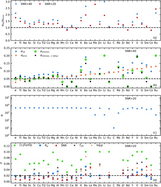
Same as Fig. 4 but for asteroseismic giants. The elements are sorted by measurement uncertainty.

Open in new tabDownload slide

To better understand as to why σ_intrinsic (abundance scatter at a given age and metallicity) in general is small, we estimated abundances by binning the stars in the ([s/Fe]–[α/Fe], [Fe/H]) plane and interpolating over the median values in each bin, with [s/Fe] = ([Ba/Fe] + [Y/Fe])/2. The estimates of σ_intrinsic were very similar but systematically lower than when estimating from abundances from age and [Fe/H]. For MSTO stars, 23 elements had σ_intrinsic less than 0.12 with a mean of 0.026. For giants stars, 24 elements had σ_intrinsic less than 0.12 with a mean of 0.035. This suggests that there are only three independent groups of elements from which most of the abundance scatter can be explained: the Fe group, the α-process group, and the s-process group.

3.3 An empirical model for abundance as a function of age and metallicity

If the Sun is a typical disc star, f_{⊙, X} should be zero because abundances are defined relative to the solar abundance. However, if the measured abundances have a dependence on stellar parameters like T_eff and log g, then f_{⊙, X} will vary depending upon the mean T_eff and log g of stars with solar age and metallicity in the studied sample. Such a dependence on stellar parameters could be due to systematics in spectroscopic analysis or due to real physical effects, such as atomic diffusion (Dotter et al. 2017; Liu et al. 2019; Souto et al. 2019).

Alternatively, the Sun might be atypical for certain elements due to the existence of rocky planet. For example, Meléndez et al. (2009) suggested that terrestrial planets might lock up refractory elements. Hence, the mean elemental abundances of solar twins that do not have rocky planets should increase with the condensation temperature of the elements. Bedell et al. (2018) investigated this with 79 solar twins and confirmed that the Sun has a mild deficiency of refractory elements. However, there are also alternate scenarios that can make the Sun apparently deficient in refractory elements. Spina et al. (2021a) have shown that planet engulfment can alter the surface composition of stars like the Sun (increase the fraction of refractory elements) that have a thin convective envelope (see also Spina et al. 2018a). Is planet engulfment common or uncommon in solar twins is not yet clear (e.g. Nibauer et al. 2021), suggesting the existence of two distinct populations. In Fig. 6, we plot the mean elemental abundance of stars as a function of the condensation temperature (Lodders 2003) for stars having the same age and metallicity as that of the Sun. The plot shows very little trend with condensation temperature. However, for elements with condensation temperature greater than 1200 K, a mild positive correlation is visible consistent with Bedell et al. (2018). Strictly speaking, to be a solar twin, a star should also have the same mass as that of the Sun, but we do not put any such restriction here. Hence, it is plausible that a significant fraction of our Sun-like stars have thicker convective envelopes and for them planet engulfment will have very little effect on their surface abundances.

Figure 6.

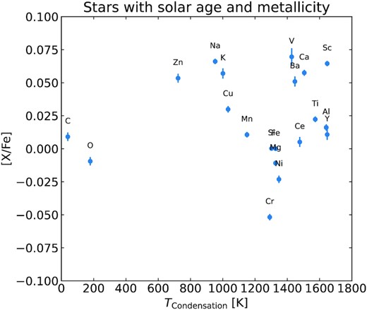
Median abundance of elements for GALAH DR3 stars with age and metallicity similar to the Sun as a function of the condensation temperature of the elements. In sum, 1000 stars with age (4.6 ± 0.58 Gyr) and metallicity (0 ± 0.057 dex) closest to the Sun were chosen. Error bar is based on the standard error of the mean.

Open in new tabDownload slide

To determine f_{[Fe/H], X} and f_{τ, X}, we adopt a non-parametric approach. The function to be determined is computed at pre-defined equispaced locations and linear interpolation is used to compute the values for any arbitrary location. We start with guess values for f_{[Fe/H], X} (based on stars with age close to solar age). Next, we alternately estimate f_{τ, X} and f_{[Fe/H], X} by computing median values of |${\rm [X/Fe]} - f_{\odot ,{\rm X}}-f_{\rm [Fe/H],{\rm X}}({\rm [Fe/H]})$| in bins of τ, and median values of [X/Fe] − f_{⊙, X} − f_{τ, X}(τ) in bins of [Fe/H], respectively.

The estimated functions f_{τ, X} and f_{[Fe/H], X} are shown as black lines in Figs 7 and 8, respectively. Also shown as dashed curves in Fig. 7 is the median abundance as a function of age for stars lying in different metallicity bins but shifted by subtracting f_{⊙, X} + f_{[Fe/H], X}. The curves for different metallicity bins closely follow the black curve corresponding to f_{τ, X}, suggesting that the dependence on age is independent of the dependence on metallicity. A similar conclusion can be reached from Fig. 8 where the dashed curves, showing the abundance dependence on [Fe/H] for stars in different age bins but shifted by subtracting f_{⊙, X} + f_{τ, X}, follow the solid black curve corresponding to f_{[Fe/H], X}. The overall dispersion with respect to values predicted by equation (3) relative to measurement uncertainty is listed in Fig. 7 (the first number at the bottom of each panel). It is very similar to the dispersion obtained using the 2D interpolation scheme in the (age,[Fe/H]) plane as shown in Fig. 3 (the number at the bottom of each panel). This demonstrates that the empirical approach (analytical functions) in spite of fewer degrees of freedom is as good as the non-parametric approach (2D interpolation).

Figure 7.

Elemental abundance f_{τ, X} of MSTO stars (S/N>10) as a function of age for different elements (solid black line). Dashed curves show the dependence with age for different bins in metallicity. A metallicity-dependent shift f_{[Fe/H], X} is applied to the dashed curves. The number on the top denotes the number of stars. The second number on the bottom denotes the overall dispersion (based on 16 and 84 percentile values) of the measured abundance as compared to abundance predicted by the model. The first number on the bottom is the overall dispersion relative to the measurement uncertainty just as in Fig. 3. The profiles are constrained to have zero abundance for stars with solar age and metallicity. The abundance for solar age and metallicity is given by the second number on the bottom.

Open in new tabDownload slide

Figure 8.

Elemental abundance f_{[Fe/H], X} of MSTO stars (S/N>10) as a function of [Fe/H] for different elements (solid black line). Dashed curves show the dependence with [Fe/H] for different bins in age. An age-dependent shift f_{τ, X} is applied to the dashed curves. The number on the top denotes the number of stars. The first number on the bottom denotes the overall dispersion (based on 16 and 84 percentile values) of the measured abundance as compared to abundance predicted by the model. The profiles are constrained to have zero abundance for stars with solar age and metallicity. The abundance for solar age and metallicity is given by the second number on the bottom.

Open in new tabDownload slide

Stars with very low [Fe/H] (less than −0.6 dex) are also the oldest stars (age greater than 11.5 Gyr; see Fig. 2a). This means that f_{[Fe/H], X} is degenerate with f_{τ, X} for the most metal-poor and the oldest stars. This, in turn, means that f_{τ, X} beyond 11.5 Gyr and f_{[Fe/H], X} below −0.6, could be inaccurate. However, their sum will still be accurate.

3.3.1 An analytical model for [α/Fe]

Figure 9.

Metallicity and age dependence of α elemental abundance. Solid blue line shows the median profile for the MSTO stars observed by GALAH and having S/N > 20, and the blue shaded region is the 16 and 84 percentile spread around it. The dashed lines are predictions of a model with, α_max = 0.225, α_outer = 0.18, F_α = −0.5, ΔF_α = 0.4, τ_α = 10.9 Gyr, and Δτ_α = 1.5, which is designed to fit the GALAH data. F stands for metallicity [Fe/H], and α_min(F) is an analytical function of metallicity as shown by the dashed line in panel (a).

Open in new tabDownload slide

The functional form of the new analytic model as given by equation (5) is different from equation (3). For an age less than 8 Gyr, both models are effectively similar. However, for an age greater than 8 Gyr, their functional form differs but their predicted values for observed stars are indistinguishable. This is because old stars are, in general, metal-poor, and this means that for old ages, the metallicity dependence of [α/Fe] is not well constrained by the data. In other words, two different models can fit the same data. To really test the difference between the two models, we need old stars with a wide range of metallicity.

3.4 Classification of elements based on their abundance trends with age and [Fe/H].

We now describe a simple scheme to classify the elements based on their trends with age and [Fe/H]. First, we compute Δ[X/Fe]/Δlog Age, the rate of change of abundance with age, using f_{τ, X} for an age of 3 and 11 Gyr. Secondly, we compute Δ[X/Fe]/Δlog [Fe/H], the rate of change of abundance with [Fe/H]), using f_{[Fe/H], X} for an [Fe/H] of −0.4 and 0.2. Next, we make a scatter plot of different elements in the gradient plane, which is shown in Fig. 10. The elements are classified based on the polar coordinate angle θ in the gradient plane. Al and Zn (θ < 45°) have a positive age gradient but a weak [Fe/H] gradient. Ni, Cr, Cu, and Mn (45° < θ < 135°) have a strong [Fe/H] gradient. They are iron-peak elements and are produced by SNe Ia. The strong gradient with [Fe/H] suggests that the contribution of SNe Ia to the production of these elements is more than that for Fe, which is about 50 per cent Kobayashi et al. (2020). Na (135° < θ < 180°) has a mild negative age gradient. Ba, Y, V, K, Zr, and Co (180° < θ < 270°) have a negative age and [Fe/H] gradient. Among these elements Ba and Y are known to be elements produced by the s-process in AGB stars. As the contribution of AGB stars increases with time, the abundance of these elements is expected to have a negative age gradient. The last group of elements are the ones lying within 270° < θ < 360° and they are produced most likely by the α and the r-process in SNe II. Such elements are expected to have a positive age gradient. The s-, α-, and r-process elements are expected to have negative [Fe/H] gradients due to the following reason. About 50 per cent of iron is produced by SNe Ia, which is not the main source of the above elements, and since we measure the abundances relative to iron, the abundances for the above elements will fall with increasing [Fe/H]. We note that the splitting shown in Fig. 10 is very simplistic and somewhat ad hoc. For example, the span of the angle θ in each group is not the same. In future, if we have more elements and better abundance precision, one could further subdivide the s, α, and iron peak groups and try to investigate the commonalities between elements belonging to those subgroups.

Figure 10.

Classification of elements based on the gradient of the abundance in the (age,[Fe/H]) plane. Probable production sites and nucleosynthetic processes are also listed.

Open in new tabDownload slide

3.5 Comparison of abundance trends of MSTO stars with that of giants

We have shown that the chemical abundances of an MSTO star can be predicted from its age and metallicity. In principle, the giants should also follow the same abundance–age–metallicity relations as the MSTO stars. However, in practice, various factors can make the giants behave differently than the MSTO stars, such as atomic diffusion (Liu et al. 2019; Souto et al. 2019), systematic surface gravity dependent effects in spectroscopic analyses, systematics in age estimates and abundance relations not being valid for all Galactocentric radii, R.

In Fig. 11, we show f_{τ, X} for the MSTO stars (blue curve) alongside that of giants (red curve) for different elements. The shaded region shows the 16 and 84 percentile spread around the relation (spread of [X/H]-f_{[Fe/H], X} − f_{⊙, X}) for stars with S/N > 40. The trends of giants are in agreement with that of the MSTO stars; the blue and red lines track each other, and the blue and the red shaded regions show good overlap. Note there are very few stars for which Rb, Li, Ru, C, and Mo can be measured in giants; hence, we exclude them from further discussion in this section. Among the elements that can be reliably measured in giants some elements show differences with respect to the MSTO stars. For elements having a non-zero slope with age; such as Al, Zn, Y, Ba, Ca, Eu, Sc, O, Ti, Si, Ce, and Mg; at the old end, the giants seem to under predict the abundances if the slope is positive and over predict the abundances if the slope is negative. This could be due to larger uncertainties in age for giants, which means that an old age bin can have significant contamination from young stars.

Figure 11.

Abundance of different elements as a function of age for MSTO (blue) and seismic giant (red) stars with S/N > 40. The solid lines shows the function f_{τ, X} as given by equation (3). The shaded region shows the 16 and 84 percentile spread around the relation (spread of [X/H]-f_{[Fe/H], X} − f_{⊙, X}) for stars with S/N > 40. The red profile is missing for C as we do not have measurements of C for giants.

Open in new tabDownload slide

In Fig. 12, we show f_{[Fe/H], X} for MSTO stars (blue curve) alongside that of giants (red curve) for different elements. Generally, there is good agreement in trends between giants and MSTO stars, except for Zn,V, Co, and Ce at the metal-poor end. Zr, La, Ti, and Mg also show some differences at the metal poor end. This could be because most of these elements also have strong dependence on either S/N, T_eff, or log g.

Figure 12.

Abundance of different elements as a function of [Fe/H] for MSTO and seismic giant stars with S/N > 40. The solid lines shows the function f_{[Fe/H], X} as given by equation (3). The shaded region shows the 16 and 84 percentile spread around the relation (spread of [X/H]-f_{τ, X} − f_{⊙, X}) for stars with S/N > 40. The red profile is missing for C as we do not have measurements of C for giants.

Open in new tabDownload slide

4 DISCUSSIONS

4.1 Comparison with other studies

Bedell et al. (2018), using solar twins (stars with T_eff, log g, and [Fe/H] similar to the Sun) showed that scatter around the abundance–age relation is small with values between 0.01 and 0.06 and the median being around 0.02 (see also Nissen 2015). These studies represent one of the most precise abundance measurements (< 0.01 dex) due to the use of line-by-line differential analyses and the spectra having high resolution and wide wavelength coverage. However, the sample size of the solar twin studies was small (79) and the data only explored stars with solar metallicity and had a limited span in age (0 to 8 Gyr) and Galactocentric radius R. Hence, it is not obvious that all Galactic stars should have a small scatter for a given age and metallicity. We explore abundances with significantly more stars that span a wide range in age, metallicity, R, and z. Our estimate of 0.033 for the abundance scatter of MSTO stars is in good agreement with the solar twin studies.

Analysis of abundance–age relations using spectra with high resolution and wide wavelength range was extended to a wider metallicity range by a number of studies (Feltzing et al. 2017; Delgado Mena et al. 2019; Casali et al. 2020). The results in general point to small abundance scatter for a given age and metallicity, although the scatter was not explicitly reported. The focus of those studies was to identify elements that correlate with age and hence could be used as clocks to date the stars. The chemical abundances were assumed to be linear functions of age and metallicity, which is only valid for thin disc stars having low [α/Fe]. Casali et al. (2020) found that for some elements, stars with Fe/H >0.1 showed a slightly different slope for the age abundance relations as compared to stars with [Fe/H] <0.1, with the element Y being a prime example. We do not find any significant difference in the abundance-age relation for the metal-rich and metal-poor stars; except for Ba, which showed a small difference. Our study has the advantage of using significantly more stars (50 000 as compared to 560); however, our abundance precision is lower, which can potentially erode small differences. It is not clear if the differences between our result for [Y/Fe] and that of Casali et al. (2020) is due to our lower abundance precision or if it is due to systematic differences between the spectroscopic analyses. In spite of the differences, their results are still consistent with the fact that abundances can be predicted to good accuracy from just age and metallicity, which is also one of our main conclusions. Lin et al. (2020) using GALAH DR2, also explored trends with age and metallicity, but like previous studies they also focused on linear relationships. Feuillet et al. (2018), using APOGEE data, also explored age–abundance trends of giants in the solar neighbourhood, but they explored trends purely with age.

Ness et al. (2019) performed a detailed analysis of the elemental abundance scatter for a large number of stars using the large-scale spectroscopic survey APOGEE. They showed that the abundance scatter for a given age and metallicity is around 0.02 dex (Recently, Yuxi et al. 2021 performed a similar analysis and reported a scatter of 0.035 dex for the low-α stars and 0.039 dex for the high-α stars.) Our abundance scatter is slightly higher (around 0.05 dex), but, overall, it is in good agreement with their results. We and Ness et al. (2019) both arrive at the same conclusion that the abundance of most elements can be predicted from just age and metallicity. We complement and extend the Ness et al. (2019) analysis in a number of ways. The abundance scatter in Ness et al. (2019) was computed for two different data sets, one having direct age estimates from asteroseismic information provided by Kepler and the other having age estimated purely from abundances using empirical relations. The data set with direct age estimates only had about 600 stars and was confined to the solar radius. The latter data set was larger (15 000 stars) and explored stars well beyond the solar radius. Using giants with asteroseismic information from K2, we here extend the analysis of direct age measurements by having a larger number of stars (4000) and by extending beyond the solar radius. Additionally, we extend the Ness et al. (2019) analysis by also exploring s- and r-process elements that have different nucleosynthetic origin. Finally, they restricted their analysis to stars with low [α/Fe], which biases the sample to show a small scatter for the α elements, while we explore stars of all [α/Fe].

4.2 Physical interpretation of the abundance trends.

Abundance trends with age and metallicity are different for different elements; some are flat, some have positive slopes, some have negative slopes, and some show non monotonic behaviour(a rise accompanied by a fall or vice versa). Trends for some of the elements can be explained by identifying the main nucleosynthetic process and the lifetime of the stars in which they are synthesized (production sites). Some of the main production sites of elements are, exploding massive star (EMS; e.g. SNe II), exploding white dwarf (EWD; e.g. SNe Ia), and AGB stars (Kobayashi et al. 2020). EMS stars have the shortest life times and are the earliest to start the chemical enrichment of the Galaxy. EWD and AGB stars have long life times ranging from 0.5 to 20 Gyr and hence they enrich the ISM over longer time-scales. The abundances of EMS elements are expected to increase with age, along with a sharp jump at around 10 Gyr due to time delay of about a Gyr between the onset of EWD and EMS (Schönrich & Binney 2009). The abundances of EMS elements are expected to fall with increasing [Fe/H] as we measure abundances relative to Fe, about 50 per cent of which is produced by EWD. The abundances of EWD elements are expected to decrease mildly with age but increase with increasing [Fe/H]. This is because Fe is produced both in EMS and EWD. The abundances of AGB elements are expected to fall as age increases, as AGB stars have the longest life times and have a significant delay time to enrich the ISM. They are also expected to fall with increasing [Fe/H] as they are not produced along with Fe. Note this is a very simplistic view of the chemical evolution in the Milky Way. In reality, nucleosynthetic yields of certain elements depend upon the metallicity and the progenitor mass of the exploding SNe.

Based on the simple model above, we now analyse the trends of different elements individually as shown in Figs 6, 8, and 10). We focus mainly on the MSTO stars, which have larger sample sizes and higher abundance precision than the giants. The elements Ni, Cr, Mn, and Cu have little variation with age but they increase strongly with [Fe/H]. The first three are iron peak elements. Like Fe, they are produced both in EWD and EMS; an increase of [X/Fe] with [Fe/H] indicates a larger contribution from EWD compared to that for [Fe/H]. Cu is an odd Z element, a rise with [Fe/H] for [Fe/H] >0, as seen here, is predicted by the Galactic chemical evolution model of Kobayashi et al. (2020). Y, Ba, and Zr are s-process elements synthesized in AGB stars, and, as expected, their abundances decrease with age and metallicity. V and Co were also found to show a behaviour similar to s-process elements, but with much weaker dependence on age; however, they also show dependence with other stellar parameters like S/N, T_eff, and log g. Mg, Si, Sc, Ca, Ti, Eu, C, and O are all even-Z EMS elements and, as expected, their abundances increase with age and decrease with metallicity.

Some elements are known to be synthesized in EMSs, however, their trends differ from that of typical EMS elements. For example, Al and Zn are EMS elements and their abundances increase with age as expected; however, unlike other EMS elements, their dependence on [Fe/H] is almost flat except for a small rise for [Fe/H] >0. Na is an EMS element, but shows a non monotonic behaviour with both age and [Fe/H]. Finally, K is also an EMS element and it decreases with [Fe/H], but it has a non-monotonic behaviour with age. The slightly peculiar behaviour of Na, Al, Cu, and K could be due to the fact that these are odd Z elements, and their yields are known to depend on the metallicity of their progenitors (Kobayashi et al. 2020).

V, Zr, Co, Ce, Nd, and La show dependence on stellar parameters like S/N, T_eff, and log g, which is not yet understood. Hence, it is difficult to interpret their abundance trends with age and [Fe/H] in any meaningful way. V and Co decrease with [Fe/H] in agreement with Kobayashi et al. (2020), but they also show a mild decrease with age, which may or may not be expected. Ce, Nd, and La behave like EMS elements (increase with age and decrease strongly with metallicity), but according to the nucleosynthetic periodic table of Kobayashi et al. (2020), they should behave like AGB elements – decrease with age and have a weak dependence on [Fe/H]. Ru, Rb, Sm, and Mo are not well measured by GALAH, hence we do not discuss their trends. Li is known to be sensitive to T_eff and log g, which makes it difficult to interpret its dependence on age and metallicity. This is because Li is destroyed below the convection zone and the amount of destruction is sensitive to T_eff and log g through a variety of factors that control the mixing of the elements (Charbonnel & Talon 2005).

Finally, it is interesting to compare our approach with that of Weinberg et al. (2019), who showed that the median trends of [X/Mg] with [Mg/H] for two populations, high [Mg/Fe] and low [Mg/Fe] are independent of Galactic location. Their result can be interpreted as follows: [X/Fe] can be predicted from just [Mg/Fe] and [Fe/H]. This works because they analysed elements that were produced by SN Ia (EWD) and core-collapse SNe (EMS) and [Mg/Fe] and [Fe/H] can effectively account for these two processes. However, elements produced by s-process cannot be predicted by just [Mg/Fe] and [Fe/H]. This is because, for an age less than 10 Gyr, the abundance of s-process elements have strong dependence on age, while [Mg/Fe] and [Fe/H] have very little dependence on age (Fig. 7).

4.3 Why are abundances a function of age and metallicity?

Fundamentally, chemical enrichment at a given location in the Galaxy depends upon the infall of fresh gas (determines the number of H atoms), the current star formation rate (number density of EMS events that inject certain elements like O and Si), and the stellar number density (number density of EWD events that inject Fe). All of these processes have a dependence on age and birth radius. This suggests that chemical abundances should also, on average, be a function of age and birth radius and should have little variation along the azimuth. We know that the ISM currently has a negative radial metallicity gradient; as it is seen in Cepheid stars (Lemasle et al. 2013), which, because of their youth, have not scattered much from their place of birth. Various other studies have also reported a radial metallicity gradient for stars close to the Galactic mid-plane (Hayden et al. 2014; Spina et al. 2021b). Most chemical evolution models also predict metallicity to fall off with birth radius (Schönrich & Binney 2009). It is likely that metallicity has been a monotonically decreasing function of radius for all ages. If so, then for a given age, the metallicity can be used to estimate the birth radius of a star (Minchev et al. 2018). Hence, the abundances of different elements should be a function of age and metallicity.

If elemental abundances are a function of age and birth radius, then the ISM should be azimuthally homogeneous. However, the extent to which the ISM is azimuthally homogeneous is not known. Stochastic chemical enrichment along with enhanced star formation along non-axisymmetric structures like spiral arms can generate abundance scatter at a given birth radius. The stochasticity can be understood as follows. Stars are born in gas clumps inside giant molecular clouds ranging in mass from 10⁴ to 10⁶ M_⊙, which condense out of the ISM (Krumholz, McKee & Bland-Hawthorn 2019). As stars form and die, they enrich the ISM around them. Different parcels of the ISM can have distinct chemical abundance patterns depending upon the correlation length of the different production sites. If the correlation length is small, a given gas parcel can have extra enrichment from a few production events, which will make its composition distinct from other parcels. This makes the chemical enrichment stochastic. If enrichment from a single production event is large, we expect large scatter in the chemical abundances of stars with a given age and [Fe/H], and vice versa if the effect is small. Below we estimate the scatter for SNe driven chemical enrichment, which is based on a calculation by Pagel (2009). For a more general treatment of stochastic enrichment, see Krumholz & Ting (2018), where they estimate the scatter to be ∼0.1 dex.

Ejecta from a single SN can extend upto 50 pc (Pagel 2009). Assuming a gas density of 0.041 M_⊙ pc⁻³ from McKee, Parravano & Hollenbach (2015), the ejecta can enrich about 2 × 10⁴M_⊙ of the ISM. A core-collapse SN ejects about 2 M_⊙ of O and increases the mass fraction of O by 10⁻⁴. To bring the oxygen mass fraction of the ISM to that of the Sun (of 0.008), 80 SNe events would be required. A Poissonian fluctuation of |$\sqrt{80}$| leads to a scatter of 0.046 dex.

The scatter estimated above will be further reduced if additional mixing processes are at work, which are suggested by some theoretical studies. Numerical simulations by Feng & Krumholz (2014) and Armillotta, Krumholz & Fujimoto (2018) suggest that gas clouds undergo homogenization due to turbulent mixing before they start forming stars, which lowers any existing scatter of abundances in the ISM. Roy & Kunth (1995) suggest that gas can be mixed on scales of (i) 1 < l/kpc < 10 azimuthally by shear-induced turbulence from differential rotation, which can mix the gas on time-scales of the order of 10⁹ yr, (ii) 0.1 < l/kpc < 1 by cloud collision, expanding shells, and differential rotation on time-scale of 10⁸ yr, and (iii) 0.001 < l/kpc < 0.1 by turbulent diffusion on time-scale of 2 × 10⁶ yr. We now compare this with the time-scale for chemical enrichment. Based on the local star formation rate, it would take 1.3 Gyr for 80 EMS events to occur in a volume of radius 50 pc. Given the long time-scale associated with stochastic enrichment, it is very likely that the mixing process will reduce the stochastic scatter of chemical abundances in the ISM.

4.4 Implications for galactic archaeology

The fact that the abundance of different elements have a small scatter when expressed in terms of age and [Fe/H] has significant implications for the field of Galactic archaeology. It makes it easier to study certain aspects of Galactic evolution, like dynamical and chemical. However, it makes it difficult to study certain other aspects, like associating stars with their birth clusters. Below we elaborate on implications for each of the above aspects in greater detail.

4.4.1 Dynamical and chemical evolution

The ability to measure age and birth radius, R_b, is useful for Galactic archaeology in a number of ways. It is useful to understand the star formation history over the whole disc, p(τ, R_b). It is also useful to understand dynamical processes like radial migration and secular heating, which requires a multidimensional data set – the distribution p(v, r|τ, R_b). For a system in equilibrium under a gravitational potential, the six-dimensional phase space distribution function f(v, r) can be expressed in terms of the three-dimensional action space distribution f(J_R, J_ϕ, J_z). Hence, the effective dimensionality for exploring the distribution p(v, r, τ, R_b) is 5. To explore this five-dimensional space comprehensively (10 bins per dimension leading to a total of 10⁵ cells) at least several million stars (50 stars in each cell so to have a Poisson uncertainty of less than 15 per cent in each cell) scattered over a wide range of R and z will be required. Upcoming large multiobject spectroscopic surveys like SDSS-V (Kollmeier et al. 2019), 4MOST (de Jong et al. 2012), WEAVE (Dalton et al. 2012), MOONS (Cirasuolo et al. 2014) are ideally suited to pursue such science.

If elemental abundances are a function age and metallicity (or R_b), then the modelling of Galactic chemical evolution becomes simpler. This is because one does not have to worry about the scatter of elemental abundances for stars having the same age and metallicity (or R_b). Also, one does not have to worry about selection functions when comparing the observed trends of abundances with age and metallicity with that of model predictions. Observationally, fewer samples of stars are required to determine the abundance relations as a function of age and [Fe/H]. This means the relations can be determined using high-precision studies of elemental abundances and ages, but spanning over a wide range of ages, metallicities, and Galactic locations. An example applying an abundance–age–metallicity relation to build a chemodynamical model with radial migration was presented in Sharma, Hayden & Bland-Hawthorn (2021). The model was successful in explaining the origin of the double sequence in the distribution of the stars in ([α/Fe],[Fe/H]) plane and also how the distribution varies with different Galactic (R, z) locations.

4.4.2 Chemically tagging stars to their star forming aggregates

An important use of abundances is to associate stars to their star-forming aggregates, an idea known as chemical tagging (Freeman & Bland-Hawthorn 2002). The most common star-forming aggregates are giant molecular gas clouds and it is thought that they are chemically homogeneous but distinct from one another. Gas clouds born at the same time and Galactocentric radius, R_b, can have distinct abundances if the correlation lengths of elements ejected from different stars (such as SNe) are small. The abundance difference between stars will then tell us about the size of the gas clouds and the physics that determines the correlation length of different production sites (Bland-Hawthorn & Sharma 2016; Ting, Conroy & Rix 2016). Based on estimates of intrinsic abundance scatter presented here and in Ness et al. (2019), an abundance precision of 0.03 or even less would be required, which makes it difficult to purse physics related to the mass distribution of clouds and the correlation length of the ejecta. Another factor that makes chemical tagging difficult is that for the set of elements that we have analysed, the abundances are strongly correlated with each other such that there are very few groups of elements that vary independent of each other. In future, it will be important to identify elements that track unique and new production sites.

5 SUMMARY AND CONCLUSIONS

Using data from the GALAH + survey, we have explored the age and metallicity dependence of the abundances of 27 elements for stars in the Galactic disc. We explored the relations with age measurements for about 50 000 MSTO stars and 4000 giants (with asteroseismic information from the NASA K2 mission), which is significantly more stars than in previous studies. To summarize, our main findings are as follows:

• Abundances of most elements are, to a good approximation, a function of age and [Fe/H] with a mean intrinsic scatter of about 0.046 dex (over 23 elements) for giants and even less for MSTO stars (0.033 dex). The abundance relations are valid for both: MSTO stars and seismic giants, in the solar neighbourhood and beyond the solar Galactocentric radius, for low and high [α/Fe] stars, for young and old stars, and for metal-rich and metal-poor stars. The elements explored include those synthesized by different independent nucleosynthetic channels, like the s, r, and α processes.

• Abundances vary smoothly with age and [Fe/H] for stars in the Galactic disc, with no special provision being required to accommodate the thick disc or high [α/Fe] stars.

• The dependence of abundance on age and [Fe/H] is largely additively separable. Chemical evolution models should help us to understand this.

• Elements can be grouped based on the direction of their abundance gradient in the (age,[Fe/H]) plane and different groups can be roughly associated with distinct nucleosynthetic production sites.

• A handful of elements (Li, Co, Zr, La, V, and Sm for dwarfs and Ba, Y, K, and V for giants) cannot be predicted reliably from age and metallicity. They could be astrophysically interesting. However, they also have strong dependencies on other variables like T_eff, log g, and S/N, and this needs to be investigated and understood in future.

The fact that the elemental abundances are a smooth function of age and metallicity and that they are additively separable in these variables is an interesting result. However, uncertainties in age and abundance could be partly responsible for this, suggesting further investigation with better precision on age and abundances.

Abundance trends for giants are similar to that of MSTO stars. Our giants explore stars beyond the solar radius, and hence these results suggest that the derived abundance relations are valid for most stars in the Galactic disc. We do see some weak trends for giants with stellar parameters like R_g, S/N, T_eff, and log g, which weakens the Galaxy-wide applicability of the relations. However, giants as compared to MSTO stars have larger uncertainty in age, [Fe/H], and abundances, which could be responsible for some of the trends with R_g, S/N, and T_eff, and this warrants further investigation.

We discussed reasons that could lead to abundances being a function of age and [Fe/H]. The primary cause for this is the fact that the number density of events that enrich the ISM are on average a function of age and birth radius. This could lead to chemical abundances being a function of age and birth radius. Assuming [Fe/H] tracks the birth radius for a given age, it follows that abundances should be a function of age and birth radius. We also explained the cause for the small intrinsic scatter in chemical abundances for a given age and [Fe/H] (or birth radius). Using a simple stochastic enrichment scheme, we show that the intrinsic scatter in abundances for a given age and birth radius is expected to be small (∼0.05), and the scatter will be even smaller if there is additional mixing in the ISM.

The fact that the abundances of different elements are a function of age and [Fe/H] and that the intrinsic scatter about these relations is small has significant implications for the field of Galactic archaeology. First, it makes it possible to estimate the age and birth radius of stars using abundances. With age and birth radius we can explore dynamical processes like scattering and radial migration, and also the star formation history in different radial zones. Secondly, it simplifies the modelling of chemical evolution, which currently is plagued by various poorly understood processes. However, the small intrinsic scatter in abundances makes it difficult to associate stars to unique star-forming clusters, as an abundance precision of less than 0.03 dex would be required.

MSTO stars, being intrinsically faint, are not easy to observe beyond the solar neighbourhood. However, it is important to verify if the abundance relations for the MSTO stars are valid beyond the solar radius. This will require performing multiobject-spectroscopy on telescopes with large diameters. Going forward, to better pin down the intrinsic scatter, the abundance precision of local MSTO samples should be improved and more stars will be required with spectra having better S/N, higher spectral resolution, and wider wavelength coverage. Also, improvements in spectroscopic analysis techniques would be required to reduce and understand the abundance systematics due to stellar parameters like T_eff and log g and stellar types like dwarfs and giants.

ACKNOWLEDGEMENTS

SS is funded by a Senior Fellowship (University of Sydney), an Australian Research Council (ARC) Centre of Excellence for All Sky Astrophysics in 3 Dimensions (ASTRO-3D) Research Fellowship and JBH’s Laureate Fellowship from the ARC. JBH’s research team is supported by an ARC Laureate Fellowship (FL140100278) and funds from ASTRO-3D. MJH is supported by an ASTRO-3D 4-yr Research Fellowship.

The GALAH Survey is supported by the ASTRO-3D, through project CE170100013. This work has made use of data acquired through the Australian Astronomical Observatory, under programs: GALAH, TESS-HERMES, and K2-HERMES. We acknowledge the traditional owners of the land on which the AAT stands, the Gamilaraay people, and pay our respects to elders past and present.

This work has made use of data from the European Space Agency (ESA) mission Gaia (https://www.cosmos.esa.int/gaia), processed by the Gaia Data Processing and Analysis Consortium (DPAC, https://www.cosmos.esa.int/web/gaia/dpac/consortium). Funding for the DPAC has been provided by national institutions, in particular the institutions participating in the Gaia Multilateral Agreement.

DATA AVAILABILITY

The data sets were derived from sources in the public domain: [https://docs.datacentral.org.au/galah/, https://gea.esac.esa.int/archive/].

REFERENCES