


ABSTRACT
This paper presents a multiwavelength investigation of the Galactic H ii region IRAS 17149 − 3916. Using the Giant Meterwave Radio Telescope, India, first low-frequency radio continuum observations at 610 and 1280 MHz for this region are presented. The ionized gas emission displays an interesting cometary morphology, which is likely powered by the early-type source, E4 (IRS-1). The origin of the cometary morphology is discussed under the framework of the widely accepted bow shock, champagne flow, and clumpy cloud mechanisms. The mid- and far-infrared data from Spitzer-GLIMPSE and Herschel-Hi-GAL reveal a complex network of pillars, clumps, bubble, filaments, and arcs suggesting the profound influence of massive stars on the surrounding medium. Triggered star formation at the tip of an observed pillar structure is reported. High-resolution ALMA continuum data show a string of cores detected within the identified clumps. The core masses are well explained by thermal Jeans fragmentation and support the hierarchical fragmentation scenario. Four ‘super-Jeans’ cores are identified which, at the resolution of the present data set, are suitable candidates to form high-mass stars.
1 INTRODUCTION
H ii regions that are an outcome of the photoionization of newly forming high-mass stars (M ≳ 8 M⊙) not only play a crucial role in understanding processes involved in high-mass star formation but also reveal the various feedback mechanisms at play on the surrounding ambient interstellar medium (ISM) and the natal molecular cloud. Numerous observational and theoretical studies of H ii regions have been carried out in the last two decades. However, dedicated multiwavelength studies of star-forming complexes add to the valuable observational data base that provide a detailed and often crucial insight into the intricacies involved.
In this work, we study the massive star-forming region IRAS 17149 − 3916. This region is named RCW 121 in the catalogue of |$\rm H{\alpha }$| emission in the Southern Milky Way (Rodgers, Campbell & Whiteoak 1960). The mid-infrared (MIR) dust bubble, S6, from the catalogue of Churchwell et al. (2006) is seen to be associated with this complex. IRAS 17149 − 3916 has a bolometric luminosity of ∼9.4 × 10⁴ L⊙ (Beltrán et al. 2006). In literature, several kinematic distance estimates are found for this complex. The near and far kinematic distance estimates range between 1.6–2.2 and 14.5–17.7 kpc, respectively (Walsh et al. 1997; Sewilo et al. 2004; Beltrán et al. 2006; Watson et al. 2010). In a recent paper, Tapia et al. (2014a) use the spectral classification of the candidate ionizing star along with near-infrared (NIR) photometry to place this complex at 2 kpc. This is in agreement with the near kinematic distance estimates and conforms to the argument of Beltrán et al. (2006) for assuming the near kinematic distance of 2.1 kpc based on the height above the Galactic plane. Based on the above discussion, we assume a distance of 2.0 kpc in this work.
This star-forming region has been observed as part of several radio continuum surveys at 2.65 GHz (Beard, Thomas & Day 1969), 4.85 GHz (Wright et al. 1994), and more recently at 18 and 22.8 GHz by Sánchez-Monge et al. (2013). Using NIR data, Roman-Lopes & Abraham (2006) detect a cluster of young massive stars associated with this IRAS source. These authors also suggest IRS-1, the brightest source in the cluster, to be the likely ionizing star of the H ii region detected in radio wavelengths. Arnal, Duronea & Testori (2008) probed the |$^{12}\rm CO$| molecular gas in the region. Based on this observation, they conclude that RCW 121 and RCW 122 are possibly unrelated star-forming regions belonging to a giant molecular complex while negating the speculation of these being triggered by Wolf–Rayet stars located in the HM 1 cluster. In the most recent work on this source, Tapia et al. (2014a) re-visit the cluster detected by Roman-Lopes & Abraham (2006). These authors also detect three bright Herschel clumps, the positions of which coincide with three of the 1.2-mm clumps of Beltrán et al. (2006).
Introducing the IRAS 17149 − 3916 complex, in Fig. 1, we show the colour composite image of the associated region. The 5.8-|$\rm \mu m$| IRAC band, which is mostly a dust tracer (Watson, Hanspal & Mengistu 2010), displays an almost closed, elliptical ring emission morphology. The extent of the bubble, S6, as estimated by Churchwell et al. (2006) traces this. The cold dust component, revealed by the Herschel 350-|$\rm \mu m$| emission, is distributed along the bubble periphery with easily discernible cold dust clumps. Ionized gas sampled in the SuperCosmos |$\rm H{\alpha }$| survey (Parker et al. 2005) fills the south-west part of the bubble and extends beyond towards south. MIR emission at 21 |$\rm \mu m$| is localized towards the south-west rim of the bubble. This emission is seen to spatially correlate with the central, bright region of ionized gas (see Fig. 2) and is generally believed to be due to the Ly α heating of dust grains to temperatures of around 100 K (Hoare, Roche & Glencross 1991).
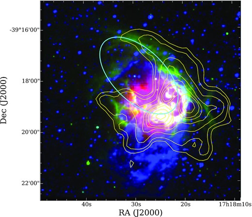
Colour-composite image towards IRAS 17149 − 3916 with the MSX 21 |$\rm \mu m$| (red), SuperCosmos |$\rm H_{\alpha }$| (blue), and IRAC 5.8 |$\rm \mu m$| (green) are shown overlaid with the contours of the Herschel 350-|$\rm \mu m$| map. The contour levels are 600, 700, 1000, 1500, 2000, 2500, 4000, and 6000 MJy/sr. The ellipse shows the position and the extent of the bubble, S6, as identified by Churchwell et al. (2006).
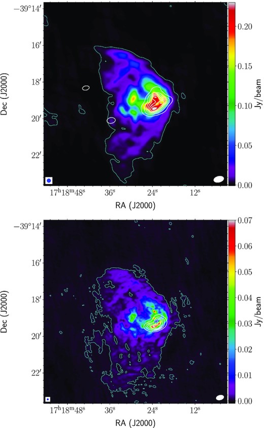
Top: 610-MHz GMRT map of the region associated with IRAS 17149 − 3916 overlaid with the 3σ (|$\sigma = 0.6\, \rm mJy\, beam^{-1}$|) level contour in light blue. White contours correspond to the 18-GHz emission mapped with ATCA (Sánchez-Monge et al. 2013), with contour levels starting from 3σ and increasing in steps of 8σ (|$\sigma = 1.2\times 10^{-2}\, \rm Jy\, beam^{-1}$|). Bottom: Same as the top panel but for 1280-MHz GMRT (|$\sigma = 0.1\, \rm mJy\, beam^{-1}$|) and 22.8-GHz ATCA map with the contour levels starting from 3σ and increasing in steps of 5σ (|$\sigma = 1.2\times 10^{-2}\, \rm Jy\, beam^{-1}$|). The GMRT maps presented here have been convolved to a resolution of 12 arcsec for 610 MHz and 5 arcsec for 1280 MHz. The beam sizes of the GMRT and ATCA maps are shown in the lower left- and right-hand corners, respectively.
In this paper, we present an in-depth multiwavelength study of this star-forming region. In discussing the investigation carried out, we present the radio observations and the related data reduction procedure followed in Section 2. This section also briefly discusses the salient features of the archival data used in the study. Section 3 presents the results obtained for the associated ionized gas and dust environment. Section 4 delves into the detailed discussion and interpretation related to the observed morphology of the ionized gas, investigation of the pillar structures, dust clumps in the realm of triggered star formation, and the nature of the detected dust clumps and cores. Section 4.5 highlights the main results obtained in this study.
2 OBSERVATION, DATA REDUCTION, AND ARCHIVAL DATA
2.1 Radio continuum observation
To probe the ionized component of IRAS 17149 − 3916, we have carried out low-frequency radio continuum observations of the region at 610 and 1280 MHz with the Giant Meterwave Radio Telescope (GMRT), Pune, India. GMRT offers a hybrid configuration of 30 antennas (each of diameter 45 m) arranged in a Y-shaped layout. The three arms contain 18 evenly placed antennas and provide the largest baseline of ∼25 km. The central |$\rm 1\, km^2$| region houses 12 antennas that are randomly oriented with shortest possible baseline of ∼100 m. A comprehensive overview of GMRT systems can be found in Swarup (1991). The target was observed with the full array for nearly full synthesis to maximize the uv coverage, which is required to detect the extended, diffuse emission. Observations were carried out during August 2014 at 610 and 1280 MHz with a bandwidth of 32 MHz over 256 channels. In the full-array mode, the resolution is ∼5 and 2 arcsec and the largest detectable spatial scale is ∼17 and 7 arcmin at 610 and 1280 MHz, respectively. Radio sources 3C 286 and 3C 48 were selected as the primary flux calibrators. The phase calibrator, 1714-252, was observed after each 40-min scan of the target to calibrate the phase and amplitude variations over the full observing run. The details of the GMRT radio observations and constructed radio continuum maps are listed in Table 1.
Details of the GMRT radio continuum observations.
| 610 MHz | 1280 MHz | |
|---|---|---|
| Date of Obs. | 2014 August 8 | 2014 August 14 |
| Flux calibrators | 3C 286, 3C 48 | 3C 286, 3C 48 |
| Phase calibrators | 1714-252 | 1714-252 |
| On-source integration time | ∼4 h | ∼4 h |
| Synth. beam | 10.69″×6.16″ | 4.41″×2.24″ |
| Position angle. (deg) | 7.04 | 6.37 |
| rms noise (mJy/beam) | 0.41 | 0.07 |
| Int. flux density (Jy) | 14.1 ± 1.4 | 12.6 ± 1.3 |
| (integrated within 3σ level) |
Astronomical Image Processing System was used to reduce the radio continuum data where we follow the procedure detailed in Das et al. (2017) and Issac et al. (2019). The data sets are carefully examined to identify bad data (non-working antennas, bad baselines, RFI, etc.), employing the tasks, TVFLG and UVPLT. Following standard procedure, the gain and bandpass calibration is carried out after flagging bad data. Subsequent to bandpass calibration, channel averaging is done while keeping bandwidth smearing negligible. Continuum maps at both frequencies are generated using the task IMAGR, adopting wide-field imaging technique to account for w-term effects. Several iterations of self-calibration (phase-only) are performed to minimize phase errors and improve the image quality. Subsequently, primary beam correction was carried out for all the generated maps.
In order to obtain a reliable estimate of the flux density, contribution from the Galactic diffuse emission needs to be accounted for. This emission follows a power-law spectrum with a steep negative spectral index of −2.55 (Roger et al. 1999) and hence has a significant contribution at the low GMRT frequencies (especially at 610 MHz). This results in the increase in system temperature, which becomes particularly crucial when observing close to the Galactic plane as is the case with our target, IRAS 17149 − 3916. The flux calibrators lie away from the Galactic plane and for such sources at high Galactic latitudes, the Galactic diffuse emission would be negligible. This makes it essential to quantify the system temperature correction to be applied in order to get an accurate estimate of the flux density. Since measurement of the variation in the system temperature of the antennas at GMRT is not automatically implemented during observations, we adopt the commonly used Haslam approximation discussed in Marcote et al. (2015) and implemented in Issac et al. (2019).
2.2 Other available data
2.2.1 Near-infrared data from 2MASS
NIR (|$\rm JHK_s$|) data for point sources around our region of interest have been obtained from the Two Micron All Sky Survey (2MASS) Point Source Catalog. Resolution of 2MASS images is ∼5.0 arcsec. We select those sources for which the ‘read-flag’ values are 1–3 to ensure a sample with reliable photometry. These data are used to study the stellar population associated with IRAS 17149 − 3916.
2.2.2 Mid-infrared data from Spitzer
The MIR images towards IRAS 17149 − 3916 are obtained from the archives of the Galactic Legacy Infrared Midplane Survey Extraordinaire (GLIMPSE) survey of the Spitzer Space Telescope. We retrieve images towards the region in the four Infrared Array Camera (IRAC; Fazio et al. 2004) bands (3.6, 4.5, 5.8, and 8.0 |$\rm \mu m$|). These images have an angular resolution of ≲2 arcsec with a pixel size of ∼0.6 arcsec. We utilize these images in our study to present the morphology of the MIR emission associated with the region.
2.2.3 Far-infrared data from Herschel
The far-infrared (FIR) data used in this paper have been obtained from the Herschel Space Observatory archives. Level 2.5 processed 70–500 |$\rm \mu m$| images from Spectral and Photometric Imaging Receiver (SPIRE; Griffin et al. 2010) and JScanam images from the Photodetector Array Camera and Spectrometer (PACS; Poglitsch et al. 2010), which were observed as part of the Herschel infrared Galactic plane Survey (Hi-GAL; Molinari et al. 2008), were retrieved. We use the FIR data to examine cold dust emission and investigate the cold dust clumps in the regions.
2.2.4 Atacama Large Millimeter Array archival data
We make use of the 1.4-mm (Band 6) continuum maps obtained from the archives of Atacama Large Millimeter Array (ALMA) to identify the compact dust cores associated with IRAS 17149 − 3916. These observations were made in 2017 (PI: A.Sanchez-Monge #2016.1.00191.S) using the extended 12-m-Array configuration towards four pointings, S61, S62, S63, and S64. Each of these pointings samples different regions of the IRAS 17149 − 3916 complex. The retrieved maps have an angular resolution of 1.4 arcsec × 0.9 arcsec and a pixel scale of 0.16 arcsec.
2.2.5 Molecular line data from MALT90 survey
The Millimeter Astronomy Legacy Team 90 GHz survey (MALT90; Foster et al. 2011; Jackson et al. 2013) was carried out using the Australia Telescope National Facility Mopra 22-m telescope with an aim to characterize molecular clumps associated with H ii regions. The survey data set contains molecular line maps of more than 2000 dense cores lying in the plane of the Galaxy, the corresponding sources of which were taken from the ATLASGAL 870-|$\rm \mu m$| continuum survey. The MALT90 survey covers 16 molecular line transitions lying near 90 GHz with a spectral resolution of 0.11 km s−1 and an angular resolution of 38 arcsec. In this study, we use the optically thin |$\rm N_2 H^+$| line spectra to carry out the virial analysis of the detected dust clumps associated with this complex.
3 RESULTS
3.1 Ionized gas
We present the first low-frequency radio maps of the region associated with IRAS 17149 − 3916 obtained using the GMRT. The continuum emission mapped at 610 and 1280 MHz is shown in Fig. 2. The ionized gas reveals an interesting, large-extent cometary morphology where the head lies in the west direction with a fan-like diffuse tail opening in the east. The tail has a north–south extension of ∼6 arcmin. The bright radio emission near the head displays a ‘horseshoe’-shaped structure that opens towards the north-east and mostly traces the south-western portion of the dust ring structure presented in Fig. 1. This is enveloped within the extended and faint, diffuse emission. In addition, there are several discrete emission peaks seen at both frequencies. The rms noise and the integrated flux density values estimated are listed in Table 1. For the latter, the flux density is integrated within the respective 3-σ contours. The quoted errors are estimated following the method discussed in Das et al. (2018).
Also included in the figure are contours showing the high-frequency ATCA observations at 18 and 22.8 GHz from Sánchez-Monge et al. (2013). These snapshot (∼10 mins) ATCA maps sample only the brightest region towards the head and the emission at 18 GHz is seen to be more extended. The GMRT and ATCA maps reveal the presence of several distinct peaks that are likely to be externally ionized density-enhanced regions thus suggesting a clumpy medium. The fact that some of these peaks could also be internally ionized by newly formed massive stars cannot be ruled out. Hence, further detailed study is required to understand the nature of these radio peaks. A careful search of the SIMBAD/NED data base rules out any possible association with background/foreground radio sources in the line of sight. Comparing with Fig. 1, the ionized emission traced in the |$\rm H{\alpha }$| image agrees well with the GMRT maps. Roman-Lopes & Abraham (2006) and Tapia et al. (2014a) present the ionized emission mapped in the Brγ line, which is localized to the central part and mostly correlates with the bright emission seen in the GMRT maps.
Assuming the radio emission at 1280 MHz to be optically thin and emanating from a homogeneous, isothermal medium, we derive several physical parameters of the detected H ii region using the following expressions from Schmiedeke et al. (2016):
Derived physical parameters of the H ii region associated with IRAS 17149 − 3916.
| Size | log NLy | EM | ne | Spectral type |
|---|---|---|---|---|
| (pc) | (cm−6pc) | (cm−3) | ||
| 3.6 | 48.73 | 5.8 × 10⁵ | 1.3 × 10² | O6.5V – O7V |
| Size | log NLy | EM | ne | Spectral type |
|---|---|---|---|---|
| (pc) | (cm−6pc) | (cm−3) | ||
| 3.6 | 48.73 | 5.8 × 10⁵ | 1.3 × 10² | O6.5V – O7V |
If we assume a single star to be ionizing the H ii region and compare the Lyman-continuum photon flux obtained from the 1280-MHz map with the parameters of O-type stars presented in table 1 of Martins, Schaerer & Hillier (2005), we estimate its spectral type to be O6.5V–O7V. This can be considered as a lower limit as the emission at 1280 MHz could be optically thick as well. In addition, one needs to account for dust absorption of Lyman continuum photons, which can be significant as shown by many studies (e.g. Paron, Petriella & Ortega 2011). The estimated spectral type suggests a mass range of ∼20−40 M⊙ for the ionizing star (Martins et al. 2005).
To decipher the nature of the ionized emission, we determine the spectral index, α, which is defined as Fν ∝ να. The flux density, Fν, is calculated from the GMRT radio maps. For this, we generate two new radio maps at 610 and 1280 MHz by setting the |$\it uv$| range to a common value of 0.14−39.7 kλ. This ensures similar spatial scales being probed at both frequencies. Further, the beam size for both the maps is set to |$\rm 12~arcsec \times 12~arcsec$|. Fν is obtained by integrating within the area defined by the 3-σ contour of the new 610-MHz map. The integrated flux density values are estimated to be |$\rm 13.7 \pm 1.3 \, Jy\,$|, |$\rm 12.1 \pm 1.2 \, Jy\,$| at 610 and 1280 MHz, respectively. These yield a spectral index of −0.17 ± 0.19. Similar values are obtained for the central, bright radio emission as well. Within the quoted uncertainties, the average spectral index is fairly consistent with optically thin, free–free emission as expected from H ii regions, which are usually dominated by thermal emission. Spectral index estimate of −0.1, consistent with optically thin thermal emission, is also obtained by combining the GMRT flux density values with the available single dish measurements at 2.65 GHz (Beard et al. 1969) and 4.85 GHz (Wright et al. 1994).
3.2 The dust environment
The warm and the cold dust emission associated with IRAS 17149 − 3916 unravels interesting morphological features like a bubble, pillars, filaments, arcs, and clumps that strongly suggest this to be a very active star-forming complex where the profound radiative and mechanical feedback of massive stars on the surrounding ISM is clearly observed. Fig. 3 compiles the MIR and FIR emission towards IRAS 17149 − 3916 from the GLIMPSE and Hi-GAL surveys. Apart from the stellar population probed at the shorter wavelengths, the diffuse emission seen in the IRAC–GLIMPSE images would be dominated by the emissions from polycyclic aromatic hydrocarbons excited by the UV photons in the photodissociation regions (Anderson et al. 2012; Paladini et al. 2012). Close to the hot stars, there would also be significant contribution from thermally emitting warm dust that is heated by stellar radiation (Watson et al. 2008). In H ii regions, emission from dust heated by trapped Ly α photons (Hoare et al. 1991) would also be present in these IRAC bands. In the wavelength regime of the 21-|$\rm \mu m$| MSX, the emission is either associated with stochastically heated very small grains (VSGs) or thermal emission from hot big grains (BGs). As we go to the FIR Hi-GAL maps, cold dust emission dominates and shows up as distinct clumps and filamentary structures where emission in the 70-|$\rm \mu m$| band is dominated by the VSGs and the longer wavelength bands like 250-|$\rm \mu m$| band trace emissions from the BGs (Paladini et al. 2012).
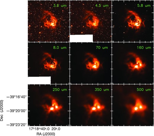
Dust emission associated with IRAS 17149 − 3916 from the Spitzer-GLIMPSE and the Herschel-Hi-GAL surveys.
3.2.1 Dust temperature and column density maps
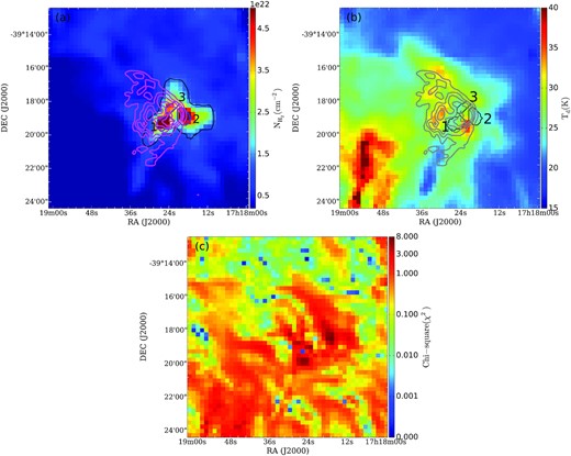
Column density (a), dust temperature (b), and chi-square (χ2) (c) maps of the region associated with the H ii region. The 610-MHz ionized emission overlaid as magenta and grey contours on column density and dust temperature maps, respectively. The contour levels are 0.01, 0.03, 0.06, 0.12, and 0.2 Jy/beam. The retrieved clump apertures are shown on the column density (in blue) and dust temperature (in black) maps following the nomenclature as discussed in the text. The black contour in (a) shows the area integrated for estimating n0 (refer Section 4.3.2.).
3.2.2 Dust clumps and cores
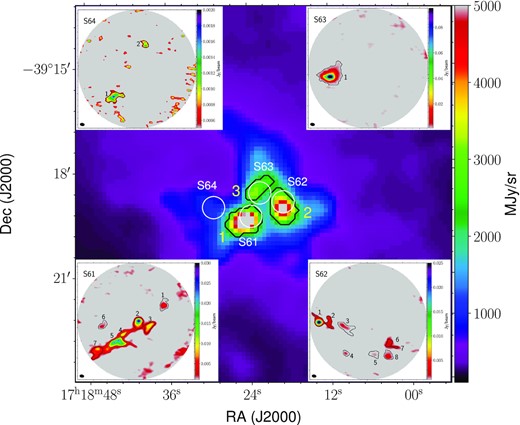
The central panel is the Herschel 350-|$\rm \mu m$| map overlaid with the Dendrogram-retrieved clump apertures in black. White circles represent four pointings of the ALMA observations, S61, S62, S63, and S64. The 1.4-mm ALMA map towards each pointing is placed at the corners of the 350-|$\rm \mu m$| image. The apertures of the dense cores extracted using the Dendrogram algorithm are overlaid and labelled on these maps. The beam sizes of the 1.4 mm maps are given towards the lower left-hand corner of each image.
Physical parameters of the detected dust clumps associated with IRAS 17149 − 3916.
| Clump | Peak position | Mean Td | ΣN(H2) | Radius | Mass | Mean N(H2) | No. density |$(n_{\mbox{H}_{2}})$| | Mvir | αvir | |
|---|---|---|---|---|---|---|---|---|---|---|
| RA (J2000) | DEC (J2000) | (K) | (× 1023 cm−2) | (pc) | (M⊙) | (× 1022 cm−2) | (× 104 cm−3) | (M⊙) | ||
| 1 | 17 18 24.32 | −39 19 28.04 | 27.8 | 6.1 | 0.3 | 250 | 5.5 | 5.0 | 452 | 1.75 |
| 2 | 17 18 18.77 | −39 19 04.54 | 25.0 | 7.1 | 0.3 | 292 | 5.4 | 5.1 | 600 | 2.15 |
| 3 | 17 18 22.57 | −39 18 36.44 | 27.3 | 2.8 | 0.2 | 117 | 3.6 | 4.6 | 450 | 4.08 |
ALMA continuum data enable investigation of the detected clumps at high resolution. In Fig. 5, we show ALMA dust continuum maps at 1.4 mm towards the four pointings marked and labelled as S61, S62, S63, and S64, where the first three pointings lie mostly within three clumps and S64 lies outside towards the east. Using the same Dendrogram algorithm, several cores are identified. The key input parameters to the Dendrogram algorithm are min_value = 3σ, min_delta = σ, and min_pix = N, where σ is the rms level and N(= 60) is the beam area of the 1.4-mm maps. In order to avoid detection of spurious cores, we retain only those with peak flux density greater than 5σ. Applying these constraints, seven cores are identified towards S61 and S62 each, one towards S63 and two towards S64.
Parameters of the detected dust cores extracted associated with IRAS 17149 − 3916.
| Core | Peak position | Flux density | Radius | Mass | ||
|---|---|---|---|---|---|---|
| RA (J2000) | DEC (J2000) | (mJy) | (pc) | (M⊙) | ||
| S61 | 1 | 17 18 23.03 | −39 19 12.95 | 9.7 | 0.01 | 1.7 |
| 2 | 17 18 23.75 | −39 19 18.47 | 62.2 | 0.02 | 10.7 | |
| 3 | 17 18 23.45 | −39 19 19.53 | 32.8 | 0.02 | 5.7 | |
| 4 | 17 18 24.17 | −39 19 22.35 | 11.2 | 0.01 | 1.9 | |
| 5 | 17 18 24.34 | −39 19 25.09 | 106.7 | 0.02 | 18.4 | |
| 6 | 17 18 24.76 | −39 19 19.50 | 4.5 | 0.01 | 0.8 | |
| 7 | 17 18 24.93 | −39 19 28.12 | 31.8 | 0.02 | 5.5 | |
| S62 | 1 | 17 18 20.38 | −39 18 54.32 | 46.0 | 0.02 | 9.4 |
| 2 | 17 18 20.09 | −39 18 54.43 | 9.8 | 0.01 | 2.0 | |
| 3 | 17 18 19.64 | −39 18 56.07 | 7.9 | 0.02 | 1.6 | |
| 4 | 17 18 19.63 | −39 19 04.70 | 2.1 | 0.01 | 0.4 | |
| 5 | 17 18 18.82 | −39 19 04.94 | 3.1 | 0.01 | 0.6 | |
| 6 | 17 18 18.35 | −39 19 01.65 | 19.2 | 0.02 | 3.9 | |
| 7 | 17 18 18.42 | −39 19 05.37 | 8.2 | 0.01 | 1.7 | |
| S63 | 1 | 17 18 23.48 | −39 18 40.70 | 357.7 | 0.03 | 62.3 |
| S64 | 1 | 17 18 29.98 | −39 19 11.22 | 7.0 | 0.02 | 1.1 |
| 2 | 17 18 29.10 | −39 18 54.11 | 1.9 | 0.01 | 0.3 | |
3.3 Molecular line observation of identified clumps
We use the optically thin |$\rm N_2 H^+$| line emission to determine the VLSR and the line width, =ΔV of the clumps. The line spectra are extracted by integrating over the retrieved apertures of the clumps as shown in Fig. 6. The |$\rm N_2 H^+$| spectra have seven hyperfine structures and the hfs method of CLASS90 is used to fit the observed spectra. The line parameters retrieved from spectra are listed in Table 5. The VLSR determined agrees well with the value of |$\rm 13.7\, km s^{-1}$| obtained from |$\rm CS(2-1)$| observations of the region by Bronfman, Nyman & May (1996).

Spectra of the optically thin N2H+ line emission extracted over the three identified clumps associated with IRAS 17149 − 3916. The red curves are the hfs fit to the spectra. The estimated VLSR is denoted by the dashed blue line and the location of the hyperfine components by magenta lines.
The retrieved |$\rm N_2 H^+$| line parameters, VLSR, ΔV, Tmb, and ∫TmbdV for the identified clumps associated with IRAS 17149 − 3916.
| Clump | VLSR | ΔV | Tmb | ∫TmbdV |
|---|---|---|---|---|
| (km s−1) | (km s−1) | (K) | (K km s−1) | |
| 1 | −13.0 | 3.2 | 1.5 | 5.4 |
| 2 | −13.8 | 3.7 | 1.6 | 6.8 |
| 3 | −13.8 | 3.9 | 0.8 | 3.1 |
| Clump | VLSR | ΔV | Tmb | ∫TmbdV |
|---|---|---|---|---|
| (km s−1) | (km s−1) | (K) | (K km s−1) | |
| 1 | −13.0 | 3.2 | 1.5 | 5.4 |
| 2 | −13.8 | 3.7 | 1.6 | 6.8 |
| 3 | −13.8 | 3.9 | 0.8 | 3.1 |
4 DISCUSSION
4.1 Understanding the morphology of the ionized gas
As seen, the GMRT maps reveal the large extent and prominent cometary morphology of the H ii region associated with IRAS 17149 − 3916, which was earlier discussed as a roundish H ii region by Tapia et al. (2014a). In this section, we attempt to investigate the likely mechanism for this observed morphology. The widely accepted models to explain the formation of cometary H ii regions are (1) the bow-shock model (e.g. van Buren & Mac Low 1992), (2) the champagne-flow model (e.g. Tenorio-Tagle 1979), and (3) the mass loading model (e.g. Williams & McKee 1997). However, subsequent studies, like those conducted by Cyganowski et al. (2003) and Arthur & Hoare (2006), find the ‘hybrid’ models, which are a combination of these, to better represent the observed morphologies.
The bow-shock model assumes a wind-blowing, massive star moving supersonically through a dense cloud. Whereas, the champagne-flow model invokes a steep density gradient encountered by the expanding H ii region around a newly formed stationary, massive star possibly located at the edge of a clump. Here, the ionized gas flows out towards regions of minimum density. In comparison, the model proposed by Williams & McKee (1997) invokes the idea of strong stellar winds mass loading from the clumpy molecular cloud and the cometary structure unfolds when a gradient in the geometrical distribution of mass-loading centres is introduced. In this model, the massive, young star is considered to be stationary as in the case of the champagne-flow model.
While observation of ionized gas kinematics is required to understand the origin of the observed morphology, in the discussion that follows, we discuss a few aspects based on the radio, column density, and FIR maps of the region associated with IRAS 17149 − 3916 along with the identification of E4 as the likely ionizing star (refer Section 4.2). Following the simple analytic expressions discussed in Das et al. (2018), we derive a few shock parameters to probe the bow-shock model. Taking the spectral type of E4 to be O6.5V – O7V as estimated from the radio flux density, and assuming it to move at a typical speed of |$\rm 10~km/s$| through the molecular cloud, we calculate the ‘standoff’ distance to range between |$\rm 2.6~arcsec (0.02~pc)~and~3.1~arcsec (0.03~pc)$|. This is defined as the distance from the star at which the shock occurs and where the momentum flux of the stellar wind equals the ram pressure of the surrounding cloud. The theoretically estimated value is significantly less than the observed distance of |$\sim \rm 84~arcsec (0.8~pc)$| between E4 and the cometary head. Taking viewing angle into consideration would decrease the theoretical estimate thus widening the disparity further. Based on the above estimations, it is unlikely that the bow-shock model would explain the cometary morphology. To confirm further, we determine the trapping parameter, which is the inverse of the ionization fraction. As the ionizing star moves supersonically through the cloud, the swept off dense shells trap the H ii region within it and its expansion is eventually inhibited by the ram pressure. Trapping becomes more significant when recombinations far exceed the ionizing photons. Studies of a large number of cometary H ii regions show the trapping parameter to be much greater than unity (Mac Low et al. 1991). For IRAS 17149 − 3916, we estimate the value to lie in the range of 3.2–3.5, which indicates either weak or no bow shock. Similar interpretations are presented in Das et al. (2018) and Veena et al. (2016). The trapping parameters obtained by these authors lie in the range of 1.2–4.3.
To investigate the other models, namely the champagne-flow and clumpy/mass loading wind models, we compare the observed spatial distribution of the dust component and the ionized gas. The FIR and column density maps presented in Section 3.2 show a complex morphology of pillars, arcs, and filaments in the region with detected massive clumps towards the cometary head. The steep density gradient towards the cometary head is evident. Without the ionized and molecular gas kinematics information, it is difficult to invoke the champagne-flow model. However, the maps do show the presence of clumps towards the cometary head, which could act as potential mass-loading centres and thus support the clumpy cloud model. Further observations and modelling are essential before one can completely understand the mechanisms at work.
4.2 Ionizing massive star(s)
Roman-Lopes & Abraham (2006) have studied the associated stellar population towards IRAS 17149 − 3916 in the NIR. Using the colour-magnitude diagram, these authors show the presence of a cluster of massive stars within the infrared nebula and suggest IRS-1 to be the likely ionizing source. In a later study, Tapia et al. (2014a) have supported this view citing the spectroscopic classification of IRS-1 as O5 – O6 by Bik et al. (2005) and consistency with the Lyman continuum photon flux estimated from the radio observations by Sánchez-Monge et al. (2013). While the spectral type estimated from the GMRT radio emission at 1280 MHz is consistent with that of IRS-1, we investigate the stellar population within the radio emission for a better understanding. In Figs 7(a) and (b), we plot the NIR colour-magnitude and colour–colour diagrams, respectively, of 2MASS sources located within the 3σ radio contour. Fig. 7(c) shows an enlarged view of the bottom left portion of Fig. 7(b) to highlight the location of the star E4 with respect to the main-sequence locus. Following the discussion given in fig. 7 in Tej et al. (2006), the colour–colour plot is classified into ‘F’, ‘T’, and ‘P’ regions. The ‘F’ region is occupied by mostly field stars or Class III sources, the ‘T’ region is for T-Tauri stars (Class II YSOs), and protostars (Class I YSOs) populate the ‘P’ region. As seen from the figures, there are 16 sources earlier than spectral-type B0 and 18 identified YSOs. The sample of identified YSOs falls in the ‘T’ region, the sources of which are believed to be Class II objects with NIR excess. Sources that lie towards the central bright, radio-emitting region are labelled in the figures with prefixes of ‘E’ for the sources earlier than B0 and ‘Y’ for the YSOs. As indicated in Fig. 7(b), early-type sources E1 and E2 are also the identified YSOs, Y1 and Y3, respectively. The coordinates and NIR magnitudes of these selected sources are listed in Table 6. Fig. 8 shows the spatial distribution of the above sources with respect to the radio and 5.8-|$\rm \mu m$| emission.
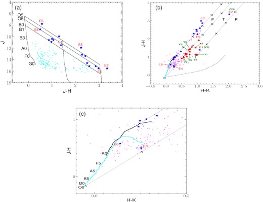
(a) J versus J–H colour-magnitude diagram of the sources (cyan dots) associated with IRAS 17149 − 3916 and located within the 3-σ radio contour. The nearly vertical solid lines represent the ZAMS loci with 0, 15, and 30 magnitudes of visual extinction corrected for the distance. The slanting lines show the reddening vectors for spectral types B0 and O5. (b) J–H versus H–K colour–colour diagram for sources (magenta dots) in the same region as (a). The cyan and black curves show that the loci of main sequence and giants, respectively, are taken from Koornneef (1983) and Bessell & Brett (1988). The locus of classical T Tauri adopted from Meyer, Calvet & Hillenbrand (1997) is shown as long dashed line. The locus of Herbig AeBe stars shown as short dashed line is adopted from Lada & Adams (1992). The parallel lines are the reddening vectors where cross marks indicate intervals of 5 mag of visual extinction. The colour–colour plot is divided into three regions, namely ‘F’, ‘T’, and ‘P’ (see text for more discussion). The interstellar reddening law assumed is from Rieke & Lebofsky (1985). The magnitudes, colours, and various loci plotted in both the diagrams are in the Bessell & Brett (1988) system. The identified early-type (earlier than B0) and YSOs candidates are highlighted as blue and red stars, respectively. Of these, the ones located towards the central, bright radio emission are labelled as ‘E’ and ‘Y’, respectively. (c) An enlarged view of the bottom left portion of (b) showing the position of spectral types on the main sequence locus. The location of the source E4 and the errors on the colour are also shown.
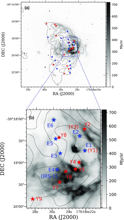
Panel a: Spitzer 5.8-|$\rm \mu m$| image in grey-scale overlaid by 610-MHz radio contours. The contour levels are 0.002, 0.01, 0.03, 0.06, 0.12, and 0.2 Jy/beam. The YSOs and massive stars detected towards the central ionized region are shown in red and blue coloured stars, respectively. Panel b: This shows the zoom-in view of central part of the H ii region.
Early-type and YSOs detected within the central, bright, radio emission of IRAS 17149 − 3916.
| Source | Coordinates | J | H | K | |
|---|---|---|---|---|---|
| RA (J2000) | DEC (J2000) | ||||
| Early-type sources | |||||
| E1 (Y1) | 17 18 22.21 | −39 18 42.24 | 11.364 | 10.039 | 8.957 |
| E2 (Y3) | 17 18 22.85 | −39 18 22.45 | 15.356 | 12.086 | 10.086 |
| E3 | 17 18 25.11 | −39 18 46.41 | 15.398 | 12.486 | 11.361 |
| E4 | 17 18 25.45 | −39 19 08.61 | 8.654 | 8.208 | 7.927 |
| E5 | 17 18 25.68 | −39 18 26.65 | 11.790 | 9.617 | 8.606 |
| E6 | 17 18 25.94 | −39 18 00.89 | 7.715 | 7.191 | 7.021 |
| YSOs | |||||
| Y1 (E1) | 17 18 22.21 | −39 18 42.24 | 11.364 | 10.039 | 8.957 |
| Y2 | 17 18 22.28 | −39 18 12.69 | 15.064 | 14.161 | 13.578 |
| Y3 (E2) | 17 18 22.85 | −39 18 22.45 | 15.356 | 12.086 | 10.086 |
| Y4 | 17 18 22.87 | −39 18 58.45 | 14.413 | 13.346 | 12.393 |
| Y5 | 17 18 23.28 | −39 19 07.77 | 12.993 | 11.906 | 11.135 |
| Y6 | 17 18 24.44 | −39 19 11.04 | 14.324 | 12.958 | 12.166 |
| Y7 | 17 18 25.14 | −39 19 25.95 | 14.741 | 13.657 | 12.664 |
| Y8 | 17 18 25.28 | −39 18 24.76 | 12.818 | 11.372 | 10.420 |
| Y9 | 17 18 28.30 | −39 19 49.71 | 14.677 | 13.449 | 12.680 |
As seen from the above analysis, in addition to the presence of possible discrete radio sources that could be internally ionized, several massive stars are also identified from the NIR colour-magnitude and colour–colour diagrams. Hence, it is likely that ionization in this H ii region is the result of this cluster of massive stars. However, the observed symmetrical, cometary morphology of the ionized emission strongly suggests that the ionization is mostly dominated by a single star. As seen in Fig. 7(a), out of the early-type sources that lie towards the central, bright radio emission, the colour and the magnitude of the source E4 are consistent with a spectral type of ∼O6. A careful scrutiny of the Fig. 7(b) shows that early-type stars E1 and E2 are embedded Class II sources and hence unlikely to be the main driving source. Sources E3, E5, and E6 are possibly reddened giants or field stars. The location of early-type star, E4 (which is the source IRS-1) in the colour–colour diagram (see enlarged view shown in Fig. 7c), agrees fairly well with the spectral-type estimate of ∼O6 obtained from the colour-magnitude diagram and strongly advocates it as the dominating exciting source. This is consistent with the identification of IRS-1 as the ionizing star in previous studies. Spatially also, the location of E4 clearly suggests its role in the formation of the network of pillar-like structures observed (see Section 4.3). As mentioned earlier, the spectral type of E4, estimated from NIR spectroscopy, is in good agreement with the radio flux. Location-wise, however, it is 30 arcsec away from the radio peak. This offset could be attributed to density inhomogeneity or clumpy structure of the surrounding, ambient ISM. Supporting this scenario of E4, being the dominant player, are the interesting pillar-like structures revealed in the MIR images discussed in the next section.
4.3 Triggered star formation
4.3.1 Pillar structures
In Fig. 9, we illustrate the identification of pillar structures in the IRAC 8-|$\rm \mu m$| image. The MIR emission presents a region witnessing a complex interplay of the neutral, ambient ISM with the ionizing radiation of newly formed massive star(s). The boxes labelled ‘A’ and ‘B’ show prominent pillar structures and the orientation of these are clearly pointed towards E4. This strongly suggests E4 as the main sculptor of the detected pillars. Furthermore, it also supports the identification of E4 as the main ionizing source of the H ii region. One of the mechanisms widely accepted to explain the formation of these pillars is the radiative-driven implosion (RDI) (Lefloch & Lazareff 1994). Here, preexisting clouds exposed to newly forming massive star(s) are sculpted into pillars by slow photoevaporation caused due to strong impingement of ionizing radiation. The other being the classical collect and collapse model of triggered star formation proposed by Elmegreen & Lada (1977). Under this framework, the expanding H ii region sweeps up the surrounding material, creating dense structures that could eventually form pillars in their shadows.
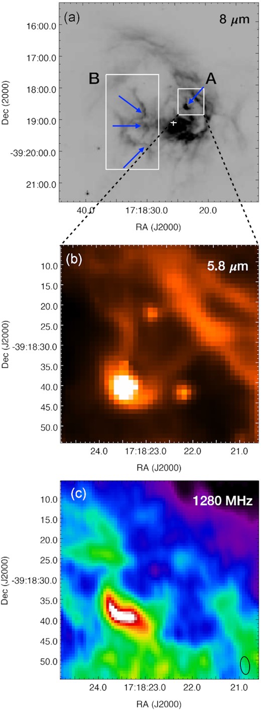
(a) 8.0-|$\rm \mu m$| map of IRAS 17149 − 3916 from the Spitzer–GLIMPSE survey. Blue arrows highlight the pillar structures identified within boxes ‘A’ and ‘B’. The white ‘ + ’ mark shows the position of E4 (IRS-1). (b) A zoom-in on ‘A’ at IRAC 5.8 |$\rm \mu m$|. (c) 1280-MHz map covering the pillar ‘A’.
Figs 9(b) and (c) show the zoomed-in IR and radio view of pillar ‘A’. Clearly seen is a slightly elongated and bright radio source at the pillar head. To ascertain the nature of the bright radio source, we estimate few physical parameters using the 1280-MHz GMRT map. Using the 2D fitting tool of CASA viewer, we fit a 2D Gaussian and determine the deconvolved size and flux density of this source to be |$\rm 19.05~arcsec \times 8.07~arcsec$| (|$\theta _{\rm source} = 12.4 \rm arcsec; 0.12 \rm pc$|) and |$\rm 445 \, mJy\,$|, respectively. Inserting these values in equations (2–4), we get logNLy = 47.30, |$n_{\rm e} = 3.9\times 10^3~\rm cm^{-3}$| and EM = |$\rm 1.8\times 10^6~pc~cm^{-6}$|. The ionized mass (|$\rm M_{ion} = \frac{4}{3}\pi \mathit{ r}^{3} \mathit {n_{\rm e}} \mathit{ m}_{p}$|, where |$\rm \mathit{ r}$| is the radius of the source and |$\rm \mathit{ m}_{p}$| is the mass of proton) is also calculated to be |$\rm 0.09 ~ \mathrm{M}_{\odot }$|. The estimated values of these physical parameters lie in between the typical values of compact and UCHII region (Kurtz 2002; Martín-Hernández, Vermeij & van der Hulst 2005; Yang et al. 2021). Hence, this radio source could well represent an intermediate evolutionary stage between a compact and an UCH ii region thus indicating a direct signature of triggered star formation at the tip of the pillar. An alternate picture for the bright radio emission at the head of the pillar could also be external ionization by the ionizing front emanating from E4. Such externally ionized, tadpole-shaped structures have been studied in the Cygnus region, where the ionized front heads point towards the central, massive Cygnus OB2 cluster (Isequilla et al. 2019). In support of the former scenario of the UCH ii region, a bright and compact 5.8-|$\rm \mu m$| emission region is seen that is co-spatial with radio emission. This compact IR emission is seen in all IRAC bands and Herschel images. While it is not listed as an IRAC point source in the GLIMPSE catalogue, it is included in the PACS 70-|$\rm \mu m$| point source catalogue (Marton et al. 2017). There also exists a 2MASS counterpart (within ∼3 arcsec) but has been excluded from the YSO identification procedure owing to poor-quality photometry in one or more 2MASS bands. It is thus likely that the compact IR emission sampled in the Spitzer–GLIMPSE and Herschel images is the massive YSO powering the UCH ii region.
Several studies (e.g. Billot et al. 2010; Paron et al. 2017) have shown evidence of star formation in the pillar tips in the form of jets, outflows, YSO population, etc. The driving mechanism for this triggered star formation, RDI, is initiated when the propagating ionizing front traverses the pillar head creating a shell (known as the ionized boundary layer, IBL) of ionized gas. If the pressure of the IBL exceeds the internal pressure of the neutral gas within the pillar head, then shocks are driven into it. This leads to compression and subsequent collapse of the clump leading to star formation. However, to comment further on the detected UCH ii region on the tip of pillar ‘A’ and link its formation to RDI, one needs to conduct pressure balance analysis using molecular line data as discussed in Paron et al. (2017) and Ortega et al. (2013). These authors have used |$\rm ^{13}CO$| transitions for their analysis, which is not possible in our case as CO molecular line data with adequate spatial resolution are not available for this region of interest. Furthermore, attempting any study with the detected MALT90 transitions is difficult, given the limited spatial resolution. In a recent study, Menon, Federrath & Kuiper (2020) have carried out involved hydrodynamical simulations to study pillar formation in turbulent clouds. As discussed by these authors, star formation triggered in pillar heads can be explained without invoking the RDI mechanism. Gravitational collapse of preexisting clumps can lead to star formation without the need for ionizing radiation to play any significant role. From their simulations, they conclude that compressive turbulence driven in H ii regions, which competes with the reverse process of photoevaporation of the neutral gas, ultimately dictates the triggering of star formation in these pillars. Further high-resolution studies are required to understand the nature of the compact radio and IR emission at the head of the pillar ‘A’.
4.3.2 Dust clumps and the collect and collapse mechanism
The detection of clumps and the signature of fragmentation to cores are evident from the FIR and sub-mm dust continuum maps presented in Fig. 5. Investigating the collect and collapse hypothesis is necessary to explain whether the dust clumps are a result of swept-up material that is accumulated or these clumps are preexisting entities. Towards this, we carry out a simple analysis and evaluate few parameters such as the dynamical age (tdyn) of the H ii region and the fragmentation time (tfrag) of the cloud.
4.4 Nature of the detected dust clumps and cores
4.4.1 Virial analysis of the dust clumps
4.4.2 Clump fragmentation and the detected cores
Hierarchical fragmentation of clumps associated with IRAS−3916.
| Clump | σth | σa | λJ | MJ | λturb | Mturb |
|---|---|---|---|---|---|---|
| (|$\rm km\, s^{-1}$|) | (|$\rm km\, s^{-1}$|) | (pc) | (M⊙) | (pc) | (M⊙) | |
| 1 | 0.3 | 1.4 | 0.2 | 6.8 | 0.8 | 543 |
| 2 | 0.3 | 1.6 | 0.2 | 5.3 | 0.9 | 807 |
| 3 | 0.3 | 1.7 | 0.1 | 5.6 | 0.8 | 819 |
| Clump | σth | σa | λJ | MJ | λturb | Mturb |
|---|---|---|---|---|---|---|
| (|$\rm km\, s^{-1}$|) | (|$\rm km\, s^{-1}$|) | (pc) | (M⊙) | (pc) | (M⊙) | |
| 1 | 0.3 | 1.4 | 0.2 | 6.8 | 0.8 | 543 |
| 2 | 0.3 | 1.6 | 0.2 | 5.3 | 0.9 | 807 |
| 3 | 0.3 | 1.7 | 0.1 | 5.6 | 0.8 | 819 |
a|$\sigma = \Delta V/\sqrt{8\, {\rm ln}2}; \Delta V$| being the |$\rm N_2 H^+$| line width.
In Fig. 10, we plot the estimated mass and radius of the identified clumps and cores. The plot also compiles several surface density thresholds proposed by various studies to identify clumps/cores with efficient and active star formation (Heiderman et al. 2010; Lada et al. 2010; Urquhart et al. 2014). In addition, criteria for these to qualify as high-mass star-forming ones are also included. All the detected clumps and cores associated with IRAS 17149 − 3916 are seen to be active star-forming regions. The three clumps satisfy the empirical mass–radius criteria, |$M \gt 870\, \mathrm{M}_\odot (r/\rm pc)^{1.33}$| defined by Kauffmann & Pillai (2010), and hence are likely to harbour massive star formation. At the core scale (|$\rm \lt 0.1~pc$|), Krumholz & McKee (2008) have posed a theoretical surface density threshold of |$\rm 1\, g\, cm^{-2}$|, below which cores would be devoid of high-mass star formation. From the figure, we see that there are four cores (2 in Clump 1, 1 each in Clumps 2 and 3) that have masses ≳10 M⊙ and above this surface density limit. These are the ‘super-Jeans’ cores discussed above. High-resolution molecular line observations are essential to shed better light on the nature of the cores, the gas kinematics involved, and for accurate determination of physical parameters like temperature, mass, etc.
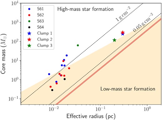
Masses of the dense cores identified from the 1.4-mm ALMA maps and the cold dust clumps identified using the 350-|$\rm \mu m$|Herschel map of IRAS 17149 − 3916 are plotted as a function of their effective radii, depicted by circles and ‘⋆’s, respectively. The shaded area corresponds to the low-mass star-forming region that does not satisfy the condition, |$M \gt 870\, \mathrm{M}_\odot (r/\rm pc)^{1.33}$| (Kauffmann & Pillai 2010). Black dashed lines indicate the surface density thresholds of 0.05 and 1 |$\rm g\, cm^{-2}$| defined by Urquhart et al. (2014) and Krumholz & McKee (2008), respectively. The red lines represent the surface density thresholds of 116 |$\mathrm{M}_\odot \, \rm pc^{-2}$| (|$\sim 0.024\, \rm g\, cm^{-2}$|) and 129 |$\mathrm{M}_\odot \, \rm pc^{-2}$| (|$\sim 0.027\, \rm g\, cm^{-2}$|) for active star formation proposed by Lada, Lombardi & Alves (2010) and Heiderman et al. (2010), respectively.
4.5 Conclusion
Using multiwavelength data, we have carried out a detailed analysis of the region associated with IRAS 17149 − 3916. The important results of this study are summarized below.
Using the GMRT, we present the first low-frequency radio continuum maps of the region mapped at 610 and 1280 MHz. The H ii region, previously believed to be nearly spherical, displays a large-extent cometary morphology. The origin of this morphology is not explained by the bow shock model. The presence of dense clumps towards the cometary head indicates either the champagne flow or the clumpy cloud model, but further observations of the ionized gas kinematics are essential to understand the observed morphology.
The integrated flux densities yield an average spectral index value of −0.17 ± 0.19 consistent with thermal free–free emission. If powered by a single massive star, the estimated Lyman continuum photon flux suggests an exciting star of spectral-type O6.5V – O7V star.
NIR colour-magnitude and colour–colour diagrams show the presence of a cluster of massive stars (earlier than spectral-type B0) located within the bright, central radio-emitting region. MIR and FIR images show complex and interesting features like a bubble, pillars, clumps, filaments, and arcs revealing the profound radiative and mechanical feedback of massive stars on the surrounding ISM.
The spatial location of source, E4 (IRS-1), and the orientation of observed pillar structures with respect to it strongly suggest it as the dominant driving source for the cometary H ii region. This view finds support from the position of E4 in the colour-magnitude and colour–colour diagrams. Further, its spectral-type estimation from literature agrees well with that estimated for the exciting source of the H ii region from GMRT data.
The column density map reveals the presence of dust clumps towards the cometary head while the dust temperature map appears to be relatively patchy with regions of higher temperature within the radio nebula. The dust clumps identified using the Herschel 350-|$\rm \mu m$| map have masses ranging between ∼100 and 300 M⊙ and radius ∼0.2–0.3 pc. Virial analysis using the |$\rm N_2 H^+$| shows that the south-east clump (#1) is gravitationally bound. For the other two clumps (# 2 and 3), the line widths would possibly have contribution from turbulence thus rendering larger values of the virial parameter.
A likely compact/UCH ii region is seen at the tip of a pillar structure oriented towards the source E4 thus suggesting evidence of triggered star formation under the RDI framework. In addition, the detected dust clumps are investigated to probe the collect and collapse model of triggered star formation. The estimated dynamical time-scales are seen to be smaller by a factor of ∼10 compared to the fragmentation time-scale of the clumps thus clearly negating the collect and collapse mechanism at work.
The ALMA 1.4-mm dust continuum map probes the dust clumps at higher resolution and reveals the presence of 17 compact dust cores with masses and radii in the range of 0.3−62.3 M⊙ and 0.01–0.03 pc, respectively. The largest and the most massive core is located within Clump 3. The estimated core masses are consistent with thermal Jeans fragmentation and support the competitive accretion and hierarchical fragmentation scenario.
Four ‘super-Jeans’ fragments are detected and are suitable candidates for forming high-mass stars and their mass and radius estimates satisfy the various threshold defined in literature for the potential high-mass star-forming cores.
ACKNOWLEDGEMENTS
We would like to thank the referee for comments and suggestions that helped in improving the quality of the manuscript. We thank the staff of the GMRT that made the radio observations possible. GMRT is run by the National Centre for Radio Astrophysics of the Tata Institute of Fundamental Research. The authors would like to thank Dr. Alvaro Sánchez-Monge for providing the FITS image of the radio maps presented in Sánchez-Monge et al. (2013). CHIC acknowledges the support of the Department of Atomic Energy, Government of India, under the project 12-R&D-TFR-5.02-0700. This work is based (in part) on observations made with the Spitzer Space Telescope, which is operated by the Jet Propulsion Laboratory, California Institute of Technology under a contract with NASA. This publication also made use of data products from Herschel (ESA space observatory). This publication makes use of data products from the Two Micron All Sky Survey, which is a joint project of the University of Massachusetts and the Infrared Processing and Analysis Center/California Institute of Technology, funded by the NASA and the NSF. This work makes use of the ATLASGAL data, which is a collaboration between the Max-Planck-Gesellschaft, the European Southern Observatory (ESO) and the Universidad de Chile. This paper makes use of the following ALMA data: ADS/JAO.ALMA#2016.1.00191.S. ALMA is a partnership of ESO (representing its member states), NSF (USA), and NINS (Japan), together with NRC (Canada), MOST and ASIAA (Taiwan), and KASI (Republic of Korea), in cooperation with the Republic of Chile. The Joint ALMA Observatory is operated by ESO, AUI/NRAO, and NAOJ. This research has made use of the SIMBAD data base, operated at CDS, Strasbourg, France.
DATA AVAILABILITY
The original data underlying this article will be shared on reasonable request to the corresponding author.
Footnotes
REFERENCES
Author notes
Present affiliation: Space Physics Laboratory, Vikram Sarabhai Space Centre, Thiruvananthapuram 695 022, Kerala, India.
