


ABSTRACT
We present a Bayesian isochrone fitting machinery to derive distances, extinctions, and stellar parameters (Teff, log g, and |$\rm [Fe/H]$|) for stars in the SkyMapper data release 3 (DR3) survey. We complement the latter with photometry from Gaia, 2MASS, and AllWISE, in addition to priors on parallaxes and interstellar extinction. We find our results to be in agreement with smaller samples of literature values derived using spectroscopic/photometric method, with typical uncertainties of order 130 K in effective temperature and 0.2 dex in surface gravity and metallicity. We demonstrate the quality of our stellar parameters by benchmarking our results against various spectroscopic surveys. We highlight the potential that SkyMapper bears for stellar population studies showing how we are able to clearly differentiate metallicities along the Gaia red (∼−0.4 dex) and blue (∼−1.1 dex) sequences using both dwarf and giant stars.
1 INTRODUCTION
In recent years, a new generation of photometric surveys are mapping the Universe. Some of these cover large areas in the sky, like Sloan Digital Sky Survey (SDSS; Alam et al. 2015), Pan-STARRS (Kaiser et al. 2002), Dark Energy Survey (The Dark Energy Survey Collaboration 2005), VISTA (Minniti et al. 2010), APASS (Henden & Munari 2014), 2MASS (Skrutskie et al.2006), and SkyMapper (Wolf et al. 2018). Other smaller scale survey are targeting specific region of the sky with filters optimized for stellar astrophysics like KIS (Greiss et al. 2012), SAGA (Casagrande et al. 2014), Pristine (Starkenburg et al. 2017), and SAGE (Zheng et al. 2018). The information obtained from these surveys is not only vital for extragalactic astronomy, they are also crucial for stellar astronomy and galactic archaeology, in particular when observing through filters designed to be sensitive to spectral features, from which we can infer stellar properties like surface temperature, gravity, and metallicity.
In addition to ground-based surveys, space-based surveys like AllWISE (Cutri et al. 2013) and Tycho2 (Høg et al. 2000) have further expanded the depth and breadth of this coverage. The biggest advantages of space-based surveys is the lack of atmospheric distortions, allowing for more precise measurements compared to ground-based telescopes, though often at the price of other technical challenges. This is especially true for Gaia (Gaia Collaboration et al. 2016a,b, 2018a), which in addition to photometry, measures positions, parallaxes, and motions for over a billion stars.
On the theoretical side, efforts are been made in stellar modelling, to provide isochrones for various combinations of chemical abundances and photometric systems across all stellar evolutionary stages. Isochrones are paths of equal time on the Hertzsprung–Russell diagram (HRD), computed from stellar evolutionary tracks (e.g. Dotter et al. 2008; Bressan et al. 2012; Choi et al. 2016), taking into account various stellar physics factors. Combining photometric information from various surveys, Gaia parallaxes, and stellar models, it is possible to derive stellar parameters (often a combination of, e.g. effective temperature, gravity, metallicity, age, and mass) on a massive scale, on the order of 108 stars (e.g. Anders et al. 2019; Green et al. 2019). These photometric parameters are complementary with the fewer (∼105–106 stars), but more precise spectroscopic parameters, provided by surveys like GALAH (Martell et al. 2017; Buder et al. 2018), APOGEE (Majewski et al. 2017), LAMOST (Zhao et al. 2012), and Gaia-European Southern Observatory (Gilmore et al. 2012). Together, they form an impressive body of data, unprecedented in its size, ready to be explored.
Adding to this repertoire, we present a Bayesian isochrone fitting machinery to derive stellar parameters, distances, and extinctions from multiband photometry. Our procedure uses the MIST isochrones (Choi et al. 2016) together with photometry from Gaia, 2MASS, AllWISE, and SkyMapper. The photometric system of the latter survey is specifically designed to be sensitive to stellar parameters, allowing us to derive reliable photometric metallicities. The SkyMapper telescope (Keller et al. 2007) is an optical wide-field survey telescope located at the Siding Spring Observatory, Australia. It has a 1.35 m primary mirror and 32 CCDs, covering a total area of 2.4 × 2.3 deg2 on the sky. SkyMapper conducts a multicolour, multi-epoch survey of the southern sky, with a filter set optimized for stellar astrophysics, delivering a uniquely powerful set of data for the investigation of stellar populations and galactic archaeology (Wolf et al. 2018). Some examples of such work include the search for metal-poor stars (Da Costa et al. 2019), the thick disc to halo transition (Sahlholdt, Casagrande & Feltzing 2019; Cordoni et al. 2021), halo blue stragglers (Casagrande 2020), the Gaia Sausage (Feuillet et al. 2020), and flaring of M dwarfs (Chang, Wolf & Onken 2020).
In this paper, we present a methodology to derive photometric stellar parameters from the SkyMapper Southern Survey DR3 (Wolf et al. 2018; Onken et al. 2019). The paper is structured as follows: In Section 2, we present the method of our analysis, in Section 3, we compare our results with a number of photometric/spectroscopic surveys, and in Section 4, we present our catalogue of stellar parameters for SkyMapper DR3, along with a case study of the Gaia red and blue sequence.
2 METHODOLOGY
2.1 Multiband photometry
In this analysis, we select up to a total of 14 bands from four photometric surveys: uvgriz from the SkyMapper Southern Sky Survey (Wolf et al. 2018; Onken et al. 2019), |$BP\, RP\, G$| from Gaia DR2 (Evans et al. 2018), JHKs from 2MASS (Skrutskie et al. 2006), and W1W2 from AllWISE (Cutri et al. 2013).
The SkyMapper uvgriz bands span a spectral range of approximately 3000–10000 Å, similar to the griz photometry of the SDSS (Fukugita et al. 1996; York et al. 2000). However, the SkyMapper u band is different from that of SDSS, and similar instead to that of the Strömgren photometric system (Strömgren 1951), which covers the Balmer discontinuity. In addition to carry sensitivity to metallic lines, the u filter traces temperature in hot stars and to gravity in AFG-type stars (e.g. Bessell 2005). Importantly, the additional v band is highly metallicity sensitive, as it covers the Ca ii doublet (Ca H at 3933.7 Å and Ca K at 3968.5 Å), which are good metallicity indicators. The SkyMapper v band in particular plays a key role in the search for extremely metal-poor stars (e.g. Keller et al. 2014; Howes et al. 2015; Nordlander et al. 2019; Chiti, Hansen & Frebel 2020).
The SkyMapper DR3 (Wolf et al. 2018; Onken et al. 2019) contains over 600 million objects with magnitudes in the range 8–22. In this study, we derive stellar parameters for an uncontaminated sample of approximately 18 million individual sources (defined as not having a next-closest Gaia EDR3 source within 5 arcsec). In our sample, all 18 million stars have at least SkyMapper uv bands, with 17.5 million stars with all six SkyMapper bands and 17.3 million stars with all 14 bands. Table 1 gives a summary of the number of stars with different bands observed. In compiling our sample, we make minimal photometric quality cuts: SkyMapper flags_psf=0 (photometry unbiased by neighbours), 2MASS gal_contam, mp_flag=0 (not contaminated by extended sources and asteroids), and AllWISE ext_flg=0 (single PSF sources only). In addition, we mask out a band if it has an uncertainty greater than 0.08 mag (for AllWISE and 2MASS) and if it has Gaia DR2 phot_bp_rp_excess_factor outside the ranges defined in Arenou et al. (2018). We discuss in Section 3 the effect of stricter quality cuts on photometry.
Summary table of number of stars with different bands present in our sample.
| Bands present | No. stars (million) |
|---|---|
| uv | 17.9 (total) |
| uvgriz | 17.5 |
| W1W2 | 17.8 |
| JHKs | 17.9 |
| |$BP\, RP\, G$| | 17.9 |
| All bands | 17.3 |
| Bands present | No. stars (million) |
|---|---|
| uv | 17.9 (total) |
| uvgriz | 17.5 |
| W1W2 | 17.8 |
| JHKs | 17.9 |
| |$BP\, RP\, G$| | 17.9 |
| All bands | 17.3 |
The isochrones used for this work are available in the Gaia DR2 system, but we update to Gaia EDR3 parallaxes (Brown et al. 2021) for distance prior. The other prior used in this work is reddening from the Schlegel, Finkbeiner & Davis (1998) map.
We apply corrections to the Gaia EDR3 parallaxes and their uncertainties to counter known systematic effects (Lindegren et al. 2021). Gaia DR2 G-band magnitudes are corrected following (Casagrande & VandenBerg 2018b, i.e. |$0.0505+0.9966\, G$| for 6 ≤ G ≤ 16.5 and G − 0.0056 for G > 16.5), to place them exactly on to the Vega system (which is assumed in the computation of synthetic colours and magnitudes of the isochrones). We exclude a handful of stars with G < 6 due to uncalibrated saturation effects at bright magnitudes. Some of the SkyMapper bands have been shown to have spatially dependent zero-point offsets (Casagrande et al. 2019). Here, we apply the latest corrections to uvgr magnitudes outlined in Huang et al. (2021). Although the effects of these corrections on the parameters we derive are small, and within their uncertainties, we found that they improve the comparison against the GALAH spectroscopic values. Since we provide stellar parameters for several million stars, these small improvements are statistically significant. In particular, the spatial dependence of zero-points becomes important when studying stellar parameters as a function of Galactic coordinates (see e.g. discussion in Casagrande et al. 2019).
2.2 Stellar parameters determination
For the overall procedure, we sample the MIST isochrones (Choi et al. 2016) to obtain the stellar parameters that best fit our observed photometric bands. The MIST isochrones (which are based on MESA stellar evolutionary models; Paxton et al. 2015) differentiate between the initial bulk composition of the stellar models (|$\rm [Fe/H]_{bulk}$|) and the present day observed surface metallicity (|$\rm [Fe/H]_{surf}$|, which is what can be measured when a star is observed e.g. through spectroscopy). The former is a fixed input parameter of the models, whereas the latter is subject to stellar mixing, gravitational settling, and atomic diffusion (Thoul, Bahcall & Loeb 1994). In our methodology we sample |$\rm [Fe/H]_{bulk}$| and treat |$\rm [Fe/H]_{surf}$| as a model prediction. We make use of the MIST stellar models with rotation included (for |$M\gt 1.2\, \mathrm{M}_{\odot }$|), up to the maximum rotational velocity of |$\rm \nu /\nu _{crit}=0.4$|.
The best-fitting parameters are found by maximizing the posterior probability |$\rm \mathit{P}$|, where we sample for evolutionary phases (EEP), age (τ), |$\rm [Fe/H]_{bulk}$|, reddening [E(B − V)], and parallax (|$\rm \varpi _{sample}$|). In MIST, EEPs are significant, physically motivated evolutionary stages identified in the stellar tracks used to build the isochrones. The spacing between these stages is then subdivided into a number of equal steps to enable accurate interpolation between evolutionary tracks even at phases when stars are evolving rapidly (Dotter 2016). The parameters |$\lbrace \rm EEP,\tau ,[Fe/H]_{bulk} \rbrace$| map uniquely into the model stellar parameters Teff, log g, and |$\rm [Fe/H]_{surf}$|, which constitute the stellar parameters derived in this paper, along with distances and extinctions.
We chose to make the distinction between |$\rm \varpi _{model}$| and |$\rm \varpi _{sample}$| to keep the notation consistent, in practice they are the same. Similarly, by comparing |$\rm \varpi _{model}$| to |$\rm \varpi _{Gaia}$|, we are effectively drawing from the |$\rm \varpi _{Gaia}$| prior.
Adopted extinction coefficients. For all filters but WISE, they are derived assuming the standard Cardelli, Clayton & Mathis (1989) extinction law. WISE coefficients are only mildly dependent on stellar parameters and the underlying extinction law.
Adopted extinction coefficients. For all filters but WISE, they are derived assuming the standard Cardelli, Clayton & Mathis (1989) extinction law. WISE coefficients are only mildly dependent on stellar parameters and the underlying extinction law.
As mentioned previously, the posterior is sampled in three steps, with each step building on the results from the previous step. The first step is a global maximization of probability across a dense MIST grid, the properties of this grid are listed in Table 3. The Python package isochrones1 is used for interpolation of the isochrones. In order to speed up the calculation, we first estimate the metallicity range of a given star using the SkyMapper metallicity calibration (Casagrande et al. 2019). We only compute |$\rm \mathit{ P}$| for the model points falling within |$\rm \pm$|1 dex of the calibration value. We then project the model points into a set of distances and reddenings to obtain their corresponding model apparent magnitudes. To construct this set, we uniformly sample five parallaxes within three standard deviations of |$\rm \varpi _{Gaia}$| and five reddenings from 0 to 1.1 × E(B − V)S, making a set of 25 possible distance/reddening combinations. Finally we compute |$\rm \mathit{ P}$| for the remaining model points at all combinations and find the best-fitting model point, distance, and reddening.
List of step sizes of the model grid. We include all evolutionary stages from zero-age main sequence (EEP 202) to thermally pulsating asymptotic giant branch (EEP 808). The varying step sizes are mainly introduced to construct an approximately uniform model grid in all dimensions.
| Parameter | Range | Step size |
|---|---|---|
| log(age; yr) | |$\rm 8.5,10.3$| | 0.06 |
| |$\rm [Fe/H]_{bulk}\ (dex)$| | |$\rm -3, -1$| | 0.04 |
| −1, 0.5 | 0.03 | |
| EEP | |$\rm 202,430$| | 10 |
| |$\rm 430,550$| | 3 | |
| 550,808 | 10 |
| Parameter | Range | Step size |
|---|---|---|
| log(age; yr) | |$\rm 8.5,10.3$| | 0.06 |
| |$\rm [Fe/H]_{bulk}\ (dex)$| | |$\rm -3, -1$| | 0.04 |
| −1, 0.5 | 0.03 | |
| EEP | |$\rm 202,430$| | 10 |
| |$\rm 430,550$| | 3 | |
| 550,808 | 10 |
The next step is to search around the best-fitting solution in case the global maximum is in between model points. Here, we use scipy.optimize and take {EEP, |$\rm \tau , [Fe/H]_{bulk}, \mathit{E}(\mathit{B}-\mathit{V}), \varpi _{sample}\rbrace$| from the previous step as starting point. scipy.optimize uses the Gao & Han (2012) implementation of the Nelder–Mead algorithm (Singer & Nelder 2009).
The third and final step is using MCMC sampling to determine the distribution of the derived parameters, again using the solution from previous step as the starting point. Here, we use the ensemble sampler emcee (Foreman-Mackey et al. 2013), deploying an ensemble of 50 walkers, with 100 burn-in steps and 300 running steps, constructing a MCMC chain of 15 000 steps in total. The ensemble sampler spreads walkers around the best-fitting solution found in step two and effectively samples the underlying distribution from different directions in the parameter space.
We take the standard deviation of the resulting distributions as internal uncertainties of our derived parameters. We consider a solution found when scipy.optimize indicates convergence and the acceptance fraction (the portion of accepted proposed steps, an indication of chain robustness) of the MCMC chain is greater than 0.1. We obtain distributions not only of the sampled parameters, but also of the ‘secondary’ stellar parameters Teff, log g, and |$\rm [Fe/H]_{surf}$|, which are actually what we are more interested in. In addition to the mean and standard deviations of the derived quantities, we also provide their covariance matrices (an example is shown in the Appendix, TableA2). We decide to use a relatively small MCMC ensemble to sample the posterior mainly to decrease computation time. In our case, a smaller ensemble will still adequately probe the shape of the posterior since the previous steps should already have located the global maximum for most stars, so it is not necessary to employ large MCMC chains to fully search the parameter space. To test this, we analyse a set of random stars using 100 walkers, 200 burn-in steps, and 500 running steps, constructing a much larger chain of 50 000 steps. We only find very minor differences in the mean and standard deviation of the large chain compared to our standard chain, with mean absolute differences being 5.5 K for temperature, 0.004 dex for gravity, and 0.0005 dex for surface metallicity.
There are a small number of our stars (|$\sim\!2\,\mathrm{ per}\,\mathrm{ cent}$|) which have negative Gaia parallaxes. In these cases, we restrict our parallax sampling to only the positive portion of the |$\rm \pm\!{3} \sigma$| distribution of |$\rm \varpi _{Gaia}$|.
3 COMPARISON TO OTHER WORKS
In order to assess the precision of our stellar parameters, as well as the dependence of stellar parameter determination on to each photometric band, we compare our results with a number of surveys. Our main comparison in Section 3.1 is with GALAH DR3 (Buder et al. 2021). GALAH is an excellent test-bed for our results because of its high-resolution, high-precision spectroscopic stellar parameters. We also use it to assess the impact of various filters on to our parameter determination (Section 3.2). Comparison with stellar parameters from other surveys is done in Section 3.3.
3.1 The SkyMapper ∩ GALAH sample
Our GALAH ∩ SkyMapper sample has approximately 330 000 stars, considering only stars with good GALAH spectroscopic parameters flag_sp=0. The top panels of Fig. 1 show the HRD using parameters derived from this work and the bottom panels show the Teff and log g comparisons between this work and GALAH. The density plot on the top-left panel shows that with our parameters we are able to reproduce well the GALAH HRD. The top-right panel in Fig. 1 shows the photometric |$\rm \chi ^2$| from the best-fitting solutions. Here, we define the photometric |$\rm \chi ^2$| according to equation (2), which is essentially an unnormalized |$\rm \chi ^2$|. Overall, the highest photometric |$\rm \chi ^2$| are found at the top of the red giant branch (RGB) and at the bottom of the main sequence: this is not surprising since cool stars are harder to model and to predict theoretical colours for. Further, intrinsically bright stars at the top of the RGB have the largest distances, and thus less precise parallaxes. The most metal-rich stars (|$\rm [Fe/H]_{surf}\ \gt\ 0.3$| dex) and high-temperature stars (Teff > 7500 K) also have high photometric |$\rm \chi ^2$|. This is likely due to the fact that hot stars have a range of rotational velocities and may impact the surface abundances, as well the possibility that for hot stars radiative acceleration alters the original chemical composition (e.g. Xiang et al. 2020).

Top panels: The HRD coloured coded in log density (left-hand panel) and photometric |$\rm \chi ^2$| (right-hand panel). Bottom panels: Log density of the comparisons between our results (y-axis) and GALAH (x-axis), for Teff (left-hand panel), log g (right-hand panel).
In terms of metallicity, the top-left panel of Fig. 2 shows the HRD colour coded in |$\rm [Fe/H]_{surf}$|. The top-right panel of Fig. 2 also shows the difference between MIST bulk and surface metallicities as a function of effective temperature. This comparison highlights the fact that in our stellar models the effect of diffusion is most significant in the effective temperature range between 6000 and 7000 K (Dotter et al. 2017). When comparing surface metallicities against GALAH, there is a small fraction of stars (around 2000) with discrepant values compared to GALAH, constituting the faint trails in the metallicity comparison (the bottom-left panel in Fig. 2). Most of these stars are of high temperature (Teff > 6500 K), where GALAH has some known issues in temperature determination (Buder et al. 2021).
![Top-left panel: HRD of the GALAH sample colour coded by the derived surface metallicity. Top-right panel: Metallicity difference ($\rm [Fe/H]_{bulk} -[Fe/H]_{surf}$) as a function of temperature. Bottom-left panel: Comparison between GALAH metallicity (x-axis) and this work (y-axis). There are two tails of larger than average metallicity differences, near 0 dex on either axes. Bottom-middle panel: Histogram of differences in metallicity in sigma level $\rm \Delta [Fe/H]/\sqrt{\sigma ^2_{[Fe/H]_{GALAH}}+ \sigma ^2_{[Fe/H]_{This\, work}}}$. Bottom-right panel: Same as bottom-left panel, but with an additional photometric $\rm \chi ^2$ cut of 20, showing improved agreement. Here, we define the photometric $\rm \chi ^2$ as equation (2) (see text for discussion).](https://oup.silverchair-cdn.com/oup/backfile/Content_public/Journal/mnras/510/1/10.1093_mnras_stab3326/1/m_stab3326fig2.jpeg?Expires=1749875595&Signature=ptASg9a3wBbJeEKQ~hFIKPNAYpXHEwoona1xtWnoAOvQ8yKjJx4bINhBdiiXXDbOI1Msh7XSee8sV0yrm3Boc5ltfGLg0ftMZZ-EgjErBtTLgb1y6EnextSG5yarYQlFIqVGdHS5pyj8Mj2G4mGBiZSPyAzaeQxzpZSAausshbfpIOTpSVEd2As9Sy5TfwjmSh4rIyzDtuZPmKp93GGDxeXTXxRSGnW3G1Tv3LeGET2bcrI7ak3-thgQLpleuKT4D9gw6YSy4WNHKp0WwO8Y7ay5f26pc78xNHEUfIOqqRalE0yGnJYh3WAlz9-bdv5DtERt2Bq9FGWfEi989uOk3w__&Key-Pair-Id=APKAIE5G5CRDK6RD3PGA)
Top-left panel: HRD of the GALAH sample colour coded by the derived surface metallicity. Top-right panel: Metallicity difference (|$\rm [Fe/H]_{bulk} -[Fe/H]_{surf}$|) as a function of temperature. Bottom-left panel: Comparison between GALAH metallicity (x-axis) and this work (y-axis). There are two tails of larger than average metallicity differences, near 0 dex on either axes. Bottom-middle panel: Histogram of differences in metallicity in sigma level |$\rm \Delta [Fe/H]/\sqrt{\sigma ^2_{[Fe/H]_{GALAH}}+ \sigma ^2_{[Fe/H]_{This\, work}}}$|. Bottom-right panel: Same as bottom-left panel, but with an additional photometric |$\rm \chi ^2$| cut of 20, showing improved agreement. Here, we define the photometric |$\rm \chi ^2$| as equation (2) (see text for discussion).
Using all stars in common with GALAH, the mean differences and standard deviations (GALAH minus this work) are: |$\Delta T_{\rm eff}=91\pm 161 \, \mathrm{K}$|, |$\Delta \log g=0.072\pm 0.113 \, \mathrm{dex}$|, and |$\rm \Delta [Fe/H]_{surf}=0.064\pm 0.214\, \mathrm{dex}$|. Using the same stars, the median uncertainties derived from our MCMC for Teff, log g, and [Fe/H]surf are 63 K, 0.054 dex, and 0.085 dex. We regard these latter values as internal uncertainties. Comparison against GALAH offers a way to estimate realistic global uncertainties under the assumption that parameters are independent and normally distributed. The median GALAH Teff, log g, and [Fe/H]surf uncertainties for the comparison sample are 95 K, 0.189 dex, and 0.085 dex, respectively. Combining these GALAH uncertainties with the standard deviations above, yields for our methodology typical global uncertainties of 130 K for Teff and 0.196 dex for |$\rm [Fe/H]_{surf}$|. We note that the logg uncertainty of GALAH is significantly larger than ours, and this is likely due to the fact that we adopt the much improved Gaia EDR3 parallaxes in comparison to those from DR2 which underpin the determination of surface gravities in GALAH. The standard deviation for the logg comparison is also smaller than expected from our and GALAH combined errors. This is indicative of the fact that for both us and GALAH surface gravities are not independent as they ultimately rely on Gaia parallaxes. When comparing with logg from APOGEE and LAMOST, the global uncertainty is on the order of 0.2 dex.
Selecting stars with photometric |$\rm \chi ^2$| lower than 20 (an arbitrary cut, composed of around 40 per cent of the sample), differences and scatter are marginally reduced to |$\Delta T_{\rm eff}=88\pm 152 \, \mathrm{K}$|, |$\Delta \log g=0.063\pm 0.096 \, \mathrm{dex}$|, and |$\rm \Delta [Fe/H]_{surf}=0.055\pm 0.192\, \mathrm{dex}$|. This comparison is shown in bottom-right panel of Fig. 2. The comparison against GALAH shows that differences in metallicity and surface gravity correlate positively with both photometric |$\rm \chi ^2$| (up to a value of ∼60), and with our internal uncertainties (up to 0.05 dex in logg and 0.2 dex in |$\rm [Fe/H]_{surf}$|). Beyond these values, differences against spectroscopic parameters plateau, suggesting that there is no further gain when cutting at larger values. Differences in Teff are instead rather independent on photometric |$\rm \chi ^2$| and internal uncertainties.
Two external factors also impact our agreement against the GALAH spectroscopic parameters. One is the photometric quality of the input bands, especially for SkyMapper. We recommend selecting stars with good photometry flags: JHKs=AAA for 2MASS, W1W2=AA for AllWISE, and at least u_flags,v_flags=0 for SkyMapper (Table 4 summarizes the parameter differences with GALAH for stars with various quality bands). The Gaia Renormalized Unit Weight Error (RUWE) also seems to play a role in the quality of the stellar parameters we derive, with a mild improvement on the agreement against GALAH for RUWE <1.4. This is likely due to the dependence of our methodology on input parallaxes, which have been shown to be less trustworthy above this threshold possibly due to binary contamination, which then could also impact our photometry (e.g. Fabricius et al. 2021).
Summary of parameter agreements (GALAH minus this work) for various photometric quality flags.
| Quality flags | ΔTeff (K) | Δlog g (dex) | |$\rm \Delta [Fe/H]_{surf}\ (dex)$| |
|---|---|---|---|
| JHKs=AAA | 98 ± 213 | 0.080 ± 0.146 | 0.060 ± 0.291 |
| JHKs!=AAA* | 135 ± 422 | 0.101 ± 0.226 | 0.272 ± 0.631 |
| uv=00 | 95 ± 195 | 0.080 ± 0.142 | 0.061 ± 0.278 |
| uv!=00 | 128 ± 368 | 0.093 ± 0.191 | 0.030 ± 0.414 |
| uvgriz=000000 | 87 ± 181 | 0.073 ± 0.132 | 0.045 ± 0.260 |
| uvgriz!=000000 | 121 ± 272 | 0.101 ± 0.191 | 0.088 ± 0.362 |
| W1W2=AA | 94 ± 165 | 0.074 ± 0.113 | 0.068 ± 0.222 |
| W1W2!=AAa | 117 ± 252 | 0.079 ± 0.129 | 0.117 ± 0.301 |
Note.
Only contains a small number of stars.
In summary, we recommend a combination of photometric |$\rm \chi ^2$|, internal MCMC uncertainties, external quality flags, and the number of bands present (discussed further below) to select stars with best parameters. All this information is provided in our catalogue.
3.2 Parameter sensitivity of various bands in relation to GALAH
Here, we investigate the sensitivity to stellar parameter of individual photometric bands by exploring how the agreement against GALAH varies when removing certain filters from our methodology.
For this exercise, we select approximately 33 000 stars with robust GALAH stellar parameters and high-quality photometric observations. This is achieved by restricting GALAH uncertainties to Teff < 200 K, log g < 0.2 dex, and |$\rm [Fe/H]_{surf}\ \lt\ 0.2$| dex and flag_sp=0. We also require zero photometry quality flags (AAA for 2MASS, AA for AllWISE, and uvgriz_flags=0 for SkyMapper), including no SkyMapper proximity flag (prox_flag), which indicates that the next closest Gaia DR2 source is further away than 15 arcsec.
This data set is first run with all bands present, to gauge their effect in comparison to GALAH. Then, seven runs are performed, each time masking out one or more filters while leaving all others present. With all 14 bands present, the mean difference and standard deviation are: |$\rm \Delta T_{\rm eff}=97\pm 137 \, \mathrm{K}$|, |$\Delta \log g=0.058\pm 0.068 \, \mathrm{dex}$|, and |$\rm \Delta [Fe/H]_{surf}=0.051\pm 0.161\, \mathrm{dex}$|. We use these values as the benchmark for the rest of the comparison when using fewer bands. The effect of removing different bands is summarized in Table 5. Mean differences are always roughly the same with the benchmark, and the informative diagnostic in this case is the standard deviation.
Summary of parameter agreements (GALAH minus this work) for various masked bands.
| Masked bands | ΔTeff (K) | Δlog g (dex) | |$\rm \Delta [Fe/H]_{surf}\ (dex)$| |
|---|---|---|---|
| None | 97 ± 137 | 0.058 ± 0.068 | 0.051 ± 0.161 |
| |$BP\, RP\, G$| | 101 ± 143 | 0.051 ± 0.077 | 0.050 ± 0.176 |
| |$u\, v$| | 100 ± 160 | 0.050 ± 0.074 | 0.052 ± 0.247 |
| |$g\, r\, i\, z$| | 99 ± 142 | 0.061 ± 0.071 | 0.062 ± 0.169 |
| |$u\, v\, g\, r\, i\, z$| | 101 ± 169 | 0.064 ± 0.078 | 0.092 ± 0.338 |
| |$J\, H\, K_s$| | 97 ± 137 | 0.058 ± 0.067 | 0.051 ± 0.161 |
| |$W1\, W2$| | 109 ± 154 | 0.066 ± 0.081 | 0.068 ± 0.181 |
Temperatures can be derived with similar precision regardless of the bands used, which is indicative of the fact that Teff is the stellar parameter which most influences colours. Also for logg, both the mean differences and their standard deviations are fairly uniform regardless of the bands used. This is because logg is mainly informed from Gaia parallaxes, which are included in every analysis. For metallicity, the SkyMapper filters, especially uv stand out to be the most informative. This is not surprising since SkyMapper uv are intermediate band filters, and sample a wavelength region dominated by several spectral lines, hence having a strong dependence on metallicity (there is also a dependence on surface gravity due to the Balmer jump; however, Gaia parallaxes are much more effective for this purpose). The other SkyMapper bands, griz, are similar to the SDSS broad-band filters, and they were designed for a broad range of science goals, including extragalactic astrophysics and supernovae search (e.g. Scalzo et al. 2017). Their broad bandwidths do not respond to metallic lines as efficiently as the uv filters. However, their inclusion still provides a slight improvement over stellar parameters. We also note that removing WISE filters deteriorates metallicity determinations. This is due to the metallicity sensitivity of molecular absorption at |$\rm 4.6\mu m$| covered by W2 (e.g. Schlaufman & Casey 2014). Lastly, Gaia and 2MASS bands are less informative because of their broad coverage encompassing many spectral features (this is especially true for the overarching G band).
3.3 Comparison with other works
In addition to GALAH, we also compare our results with spectroscopic parameters from APOGEE DR16 (Ahumada et al. 2020) and LAMOST DR6 (Luo et al. 2015), photometric stellar parameters from StarHorse (SH; Anders et al. 2019), reddening values from Bayestar (Green et al. 2019), and distances from Bailer-Jones et al. (2021) and Kudritzki, Urbaneja & Rix (2020). We select a random sample of 5 million (out of 18 million), which then we cross-match with the aforementioned surveys for the comparison below.
The overlap with APOGEE is the smallest, containing only approximately 6400 stars, with the APOGEE parameter flag being zero (ASPCAPFLAG=0). The middle panels of Fig. 3 show the comparison with temperature (left-hand panel), surface gravity (middle panel), and surface metallicity (right-hand panel). The agreement (APOGEE minus this work) is very good between the two samples, with |$\Delta T_{\rm eff}=76\pm 179\, \mathrm{K}$|, |$\Delta \log g=0.146\pm 0.264\, \mathrm{dex}$|, and |$\rm \Delta [Fe/H]_{surf}=0.033\pm 0.280\,dex$|.
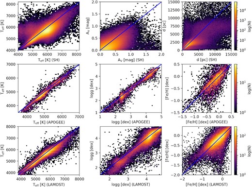
Top panels: Comparison with SH temperature (left-hand panel), AV (middle panel), and distance (right-hand panel). There are approximately 50 000 stars with negative SH AV which have been omitted in the middle panel. Middle panels: Comparison with APOGEE temperature (left-hand panel), surface gravity (middle panel), and surface metallicity (right-hand panel), 6400 stars. Bottom panels: Comparison with LAMOST temperature (left-hand panel), surface gravity (middle panel), and surface metallicity (right-hand panel), 76 000 stars.
The LAMOST2 overlap contains approximately 76 000 stars (bottom panel of Fig. 3). We note here that LAMOST and SkyMapper are located in different hemispheres, hence their overlap is quite small, despite both surveys having millions of entries. We have good temperature agreement between the two samples: |$\Delta T_{\rm eff}=105\pm 196\, \mathrm{K}$|. In terms of log g, there is some discrepancy, especially towards higher gravity, where an ‘s’-like shape can be observed. This is likely due to the LAMOST main sequence having an upward lump at near |$T_{\rm eff}=4500\, \mathrm{K}$|, as this area of the HRD is hard to define spectroscopically without the aid of Gaia parallaxes. The mean difference for gravity is |$\Delta \log g=0.115\pm 0.252 \, \mathrm{dex}$|. Similarly, for metallicity, there is a large portion of stars which we predict to be more metal-poor than LAMOST. These stars are mainly concentrated in the main sequence, where our gravity estimates are also on average higher than those of LAMOST. The resulting mean metallicity difference is |$\rm \Delta [Fe/H]_{surf}=0.022\pm 0.293\, \mathrm{dex}$|.
There are approximately 1.1 million stars in common with SH and having zero SH flags (SH_OUTFLAG=00000, the general purpose quality flag). The top panels of Fig. 3 show the comparison for temperature (left-hand panel), extinction (AV, middle panel), and distance (right-hand panel). Our extinction values are found by AV = 3.1 × E(B − V). We note, however, that the reddening law underlying SH is different from the one we adopt, and this has a systematic effect on the reddening values we derive compared to theirs. We use the inverse of our parallaxes to derive distances to compare against SH. In general, we find reasonable agreement between the two samples, mean differences and standard deviations (SH minus this work) being: |$\Delta T_{\rm eff}=215\pm 304 \, \mathrm{K}$|, |$\Delta A_{\rm V}=0.132\pm 0.178\, \mathrm{mag}$|, and |$\Delta d= -321\pm 1188\, \mathrm{pc}$| (up to 20 kpc). SH consistently has higher temperatures, larger extinctions, and smaller distances than this work. We note the presence of a cluster of stars (∼6000) for which we derive much higher temperatures than those of SH. In our sample, they are located in the turnoff region, whereas in SH, they are in the main sequence. We speculate this is largely due to the different logg estimates between the two samples: Gaia EDR3 parallax used in our analysis and DR2 parallax used in SH. For distances, the agreement is the best for nearby stars (|$\rm \lt 2\, kpc$|), where the agreement improves to |$\rm -23\pm 391\, pc$|.
Top panel of Fig. 4 shows in Galactic coordinates the stars in our 5 million random sample, colour coded by our estimated reddening values. As expected, reddening increases as we approach the Galactic plane, and we see the filamentary structure of the dust distribution projected across the Galaxy. The left-bottom panel shows the comparison between our reddening and that of Bayestar2019 (rescaled as described in Green et al. 2019) for approximately 3.3 million stars in common, the mean difference between the two sets is −0.004 |$\rm \pm$| 0.087 mag showing good consistency. Also in this case, we remark the different extinction laws used in our work and Bayestar2019.

Top panel: The Galaxy colour coded in the bi-dimensional reddening map derived from our approach. The white areas have no SkyMapper coverage, and the two white blobs at longitude around 280○ are the Small and Large Magellanic Clouds. Bottom-left panel: Comparison between E(B−V) derived using our approach and the values in Bayestar at the same distance. Bottom-middle panel: HRD of the random 5 million SkyMapper stars, colour coded in surface metallicity, showcasing our catalogue. Bottom-right panel: HRD colour coded in log density.
In addition to compare distances to SH as previously discussed, the left-hand panel of Fig. 5 shows the comparison against Bailer-Jones et al. (2021). Similar to SH, our distances compare well with Bailer-Jones et al. (2021) for both geometric and photogeometric estimates. For nearby stars (below 2 kpc), the mean differences are Δd = 112 ± 724 pc for geometric and Δd = 109 ± 776 pc for photogeometric. The differences diverge at afar, with Δd = −460 ± 1844 pc for geometric and Δd = −527 ± 1910 pc for photogeometric, up to 20 kpc.
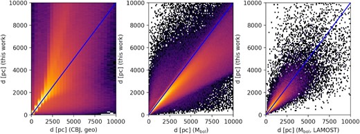
Left-hand panel: Distance comparison between our results and geometric estimates from Bailer-Jones et al. (2021; CBJ). Middle panel: Distance comparison between our parallax (y-axis) and distance inferred from |$\it{M}_{\mathrm{bol}}$| (x-axis), using our stellar parameters for the flux-weighted gravity. Right-hand panel: Same as middle panel, but with distance inferred from |$\mathit{M}_{\mathrm{bol}}$| (x-axis), using instead LAMOST parameters. All densities are in log scale.
We speculate the main reason for the differences between our distances and those in the aforementioned studies stem from the different approaches used. For this work, we derive distances by sampling from a distribution of parallaxes encompassing ±3σ of the Gaia value and its uncertainty. This means that at small parallaxes, we uniformly sample a large range of distances. In Bailer-Jones et al. (2021), a spatial density prior is used, with increasing effect at larger distances (whereas we assume no prior). These factors combine in increasing the divergence at larger distances. Although one would assume that photogeometric distances would yield a closer agreement with our analysis, but for our cross-matched sample, the difference between photogeometric and geometric distances is only |$\rm -71\pm 596$| pc, a difference too small to be distinguishable in our comparison.
As an additional check, we calculate distances from flux-weighted gravity. Kudritzki et al. (2020) show a tight correlation between the bolometric magnitude (|$\mathit{M}_{\mathrm{bol}}$|) and the stellar flux-weighted gravity (|$\rm \mathit{ g}_{F} \equiv \mathit{ g}/\mathit{T}_{\mathrm{eff}}^{4}$|), hence providing a direct way of inferring |$\mathit{M}_{\mathrm{bol}}$| from fundamental stellar physics.
Following the procedure outlined in Kudritzki et al. (2020, their equation 2), we calculate for each star the absolute bolometric magnitude |$\mathit{M}_{\mathrm{bol}}$| via flux-weighted gravity, using the effective temperature and surface gravity derived with our methodology. Assuming the |$\mathit{M}_{\mathrm{bol}}$| so derived as the ‘true’ value, when combined with an apparent magnitude and bolometric correction, we can then extract a parallax (hence a distance) to compare with ours (their equation 8). To this purpose, we employ the same procedure as in Kudritzki et al. (2020). We use WISE W1 apparent magnitudes together with their functional form for bolometric corrections, which is only a function of Teff. The advantage of using W1 is twofold. From one side, it is only a little affected by reddening which is not taken into account for this comparison. Also, the functional form for bolometric corrections in W1 can be fit well only as a function of Teff, without any dependence on other stellar parameters (equation 9 in Kudritzki et al. 2020).
The middle panel of Fig. 5 shows the comparison between distance inferred from |$\mathit{M}_{\mathrm{bol}}$| derived as described above, and our inverse sampled parallax distance. There is overall good agreement, indicating that our distances are consistent with our stellar parameters used to derive |$\mathit{M}_{\mathrm{bol}}$| via flux-weighted gravity. The mean difference is |$\rm 106\pm 225$| pc below 2 kpc and |$\rm 687\pm 1376$| pc up to 20 kpc. The right-hand panel of Fig. 5 shows a similar plot, but with distances derived using LAMOST Teff and log g to derive |$\mathit{M}_{\mathrm{bol}}$| via flux-weighted gravity. Also in this case, there is excellent agreement with the mean difference being |$\rm 73\pm 354$| pc below 2 kpc and |$\rm 60\pm 1016$| pc up to 20 kpc. Finally, we repeat this exercise with the larger GALAH sample and find similar results.
4 THE SKYMAPPER CATALOGUE
Our SkyMapper sample contains almost 18 million stars which satisfy our convergence criteria (defined as convergence during the optimization step and having a robust MCMC chain). An excerpt of the catalogue is shown in the Appendix (Table A1). In addition to the derived stellar parameters, we also provide the photometric quality flags for the selection of the best parameters (see Section 3.1 for a detailed discussion on selecting the best parameters).
4.1 The Gaia red and blue sequence in SkyMapper
As an application of our results, we study the metallicity distribution of the red and blue sequence on the HRD of high-tangential velocity stars discovered by Gaia (Gaia Collaboration et al. 2018b). The red and blue sequences are two population of stars on the HRD, separated about 0.1 mag in colour (Gaia Collaboration et al. 2018b). Although stars with tangential velocities (|$\rm \gt $|200 km s−1) have been typically regarded as members of the halo (e.g. Bensby, Feltzing & Oey 2014), the recent consensus is that the two sequences represent two different populations. The metal-poor blue sequence consists of halo stars from one or multiple accretion events (e.g. Belokurov et al. 2018; Haywood et al. 2018; Helmi et al. 2018; Kruijssen et al. 2019), whereas the metal-rich red sequence consists of the high tangential velocity, kinematically hot tail of the thick disc (e.g. Di Matteo et al. 2019; Sahlholdt et al. 2019).
For our sample, we calculate the tangential velocity as |$\rm \mathit{ v}_{T}=4.74/\varpi \sqrt{\mu ^2_{\alpha *}+\mu ^2_{\delta }}$|, where |$\mu ^2_{\alpha *}$| and |$\mu ^2_{\delta }$| are the Gaia proper motions in RA and Dec, |$\rm \varpi$| is the parallax derived from this work. The left-hand panel of Fig. 6 shows the HRD in log density, along with four boxes on the RGB and the main sequence which we use to select stars belonging to the red and blue sequence, in a fashion similar to Sahlholdt et al. (2019). The middle panel of Fig. 6 shows the metallicity distribution of the sequences, split into giants and dwarfs. We observe a clear bimodal distribution, with the overall blue sequence being more metal poor, peaking at roughly −1.1 dex and the overall red sequence peaking at roughly −0.4 dex. Overall, we qualitatively agree with previous results, but with a much larger sample of stars (e.g. Gaia Collaboration et al. 2018b; Sahlholdt et al. 2019). The separation in metallicity between the two sequences extends from the RGB, down to the main sequence (right-hand panel in Fig. 6). The giant/dwarf subpopulations within each sequence have consistent metallicities, with the blue sequence peaking at |$\rm -1.105 \pm 0.006 (\sigma =0.461$|) dex and |$\rm -1.087\pm 0.004 (\sigma =0.338$|) dex, whereas the red sequence peaks at |$\rm -0.491\pm 0.004 (\sigma =0.248$|) dex, |$\rm -0.378\pm 0.005 (\sigma =0.260$|) dex (with the uncertainties being the standard errors of the mean and the scatter the standard deviation). Metallicities of dwarfs are systematically slightly higher than in giants, in particular for the red sequence. At this stage we do not speculate whether this is due to systematics in our method, or from Galactic metallicity gradients (dwarf stars being intrinsically fainter and hence preferentially closer than giant stars). We confirm the metal-poor nature of the blue halo sequence with a metallicity scatter some 30 per cent to 80 per cent higher than in the red sequence. This might be indicative of the many metal-poor populations which have contributed to build the halo (e.g. Casagrande 2020; Naidu et al. 2020). We find that the red sequence has a peak metallicity closer to disc stars, similar e.g. to what has been obtained from other studies based on isochrone-based metallicities (Hallakoun & Maoz 2021). In a future paper, we plan delve deeper into the properties and kinematics of this sample.
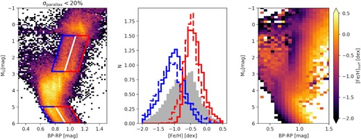
Left-hand panel: Log density plot of the HRD. Colours and absolute magnitudes are computed using both distances and reddening derived with our methodology. Approximately 100 000 stars with Gaia parallax uncertainty lesser than 20 per cent are included in this plot. Middle panel: Normalized metallicity distribution of the sequences, the grey distribution represents the overall metallicity of the sample, with the dashed distributions being the giants and the solid distributions being the dwarfs. Right-hand panel: The HRD coloured coded in derived metallicity.
5 CONCLUSION
In this paper, we construct a Bayesian isochrone fitting machinery to derive distances, extinctions, and stellar parameters (Teff, log g, and |$\rm [Fe/H]_{surf}$|) for nearly 18 million stars from SkyMapper DR3. A total of 14 photometric bands across four surveys (SkyMapper, Gaia, 2MASS, and AllWISE) are used in our analysis. In all, there are 17.3 million stars with all 14 bands of photometry. In addition, we incorporate Gaia EDR3 parallaxes and interstellar extinctions. The median internal uncertainties are 63 K for Teff, 0.054 dex for log g, and 0.082 dex for |$\rm [Fe/H]_{surf}$|, comparing our results with spectroscopic surveys yields global uncertainties on the order of 130 K for Teff, 0.2 dex for log g, and |$\rm [Fe/H]_{surf}$|.
MIST isochrones allow us to make a distinction between bulk and surface metallicities. In the sampling, |$\rm [Fe/H]_{bulk}$| is treated as a model input and we compare the resulting |$\rm [Fe/H]_{surf}$| to the corresponding surface abundances measured by spectroscopic surveys. We derive the uncertainties in our stellar parameters by MCMC sampling. We primarily compare our results with the GALAH DR3 survey, and find generally good agreements, with some exceptions for hot stars. Using the GALAH overlap, we investigate the parameter sensitivity of the various photometric bands used in the analysis. As expected, we find the SkyMapper uvgriz to be the most informative to metallicity. This is mainly due to the location and narrow bandwidth of the uv filters. AllWISE photometry also has metallicity sensitivity, whereas Gaia bands are very broad and mostly sensitive to Teff only.
Besides GALAH, we compare our stellar parameters with APOGEE, LAMOST, and SH, all with generally agreeable results. We also find good comparisons with Bayestar in terms of extinction. For distance, our sampled parallaxes compare well with those of Gaia EDR3, but small differences at low parallaxes imply large differences once inverted to distances. Similarly, we find compatible distances with Bailer-Jones et al. (2021), up to 2 kpc. This is the radius within which Gaia parallaxes have a typical precision on the order of ∼10 per cent, and distances can be obtained by parallax inversion without introducing significant biases. For lower precision the prior used in Bailer-Jones et al. (2021) becomes dominant. To gauge further into this, we also investigate a more direct way of inferring distances using flux-weighted gravity and find the agreement is improved compared to Bailer-Jones et al. (2021). This method also demonstrates our stellar parameters are consistent with the derived distances. Lastly, we show the metallicity distribution function of the Gaia red and blue sequence at high tangential velocity, as a quick illustration of the data. Further exploration of the kinematic aspects of this data set will be presented in a future paper.
ACKNOWLEDGEMENTS
We thank Chris Onken for helping with the SkyMapper data, and the referee for their valuable comments and suggestions which have helped to improve the paper. LC is the recipient of the Australian Research Council (ARC) Future Fellowship FT160100402. Parts of this research were conducted by the ARC Centre of Excellence ASTRO 3D, through project No. CE170100013. The national facility capability for SkyMapper has been funded through ARC LIEF grant LE130100104 from the ARC, awarded to the University of Sydney, the Australian National University, Swinburne University of Technology, the University of Queensland, the University of Western Australia, the University of Melbourne, Curtin University of Technology, Monash University, and the Australian Astronomical Observatory. SkyMapper is owned and operated by The Australian National University’s Research School of Astronomy and Astrophysics. The survey data were processed and provided by the SkyMapper Team at ANU. The SkyMapper node of the All-Sky Virtual Observatory (ASVO) is hosted at the National Computational Infrastructure. Development and support of the SkyMapper node of the ASVO has been funded in part by Astronomy Australia Limited and the Australian Government through the Commonwealth’s Education Investment Fund and National Collaborative Research Infrastructure Strategy, particularly the National eResearch Collaboration Tools and Resources and the Australian National Data Service Projects.
DATA AVAILABILITY
The data underlying this article can be found at https://www.mso.anu.edu.au/~jlin/archive/smdr3_res/.
Footnotes
isochrones.readthedocs.io
Data taken from http://dr6.lamost.org/.
REFERENCES
APPENDIX A: Catalogue example
An example table of our catalogue. Here, the uncertainties reflect internal precision only. Photometric |$\rm \chi ^2$| is defined using equation (2), which is essentially an unnormalized |$\rm \chi ^2$|. The last column indicates the number of bands present in the analysis, with 0 being present and 1 being missing. Stars with best parameters should be selected using a combination of photometric |$\rm \chi ^2$|, uncertainty, number of bands present, and external quality flags (photometric/parallax quality flags), see Section 3.1 for details. This additional information is included in the online version of this table.
| Gaia EDR3 source ID | Teff | |$\rm \sigma \mathit{T}_{\mathrm{eff}}$| | |$\rm \log \mathit{g}$| | |$\rm \sigma \log \mathit{g}$| | |$\rm [Fe/H]$| | |$\rm \sigma [Fe/H]$| | |$\rm \varpi$| | |$\rm \sigma \varpi$| | E(B−V) | |$\rm \sigma$|E(B−V) | Photometric |$\rm \chi ^2$| | Band flag |
|---|---|---|---|---|---|---|---|---|---|---|---|---|
| (K) | (K) | (dex) | (dex) | (dex) | (dex) | (mas) | (mas) | (mag) | (mag) | |||
| 4138089840248250752 | 6032 | 38 | 4.32 | 0.02 | −0.10 | 0.03 | 2.22 | 0.04 | 0.41 | 0.008 | 110.1 | 00000000000000 |
| 4345098777053035520 | 5477 | 50 | 4.26 | 0.03 | −0.03 | 0.02 | 2.07 | 0.01 | 0.25 | 0.001 | 42.4 | 00000000000000 |
| 4377847662165957888 | 5422 | 26 | 4.51 | 0.05 | 0.13 | 0.03 | 3.75 | 0.03 | 0.21 | 0.006 | 43.8 | 00000000000000 |
| 4378891648457313408 | 5419 | 20 | 3.87 | 0.02 | −0.12 | 0.02 | 1.72 | 0.05 | 0.18 | 0.005 | 12.8 | 00010000000000 |
| 4382480763646637440 | 5232 | 17 | 4.57 | 0.01 | 0.05 | 0.03 | 2.94 | 0.04 | 0.14 | 0.004 | 33.0 | 00011000000000 |
An example covariance matrix for the star 5220895866301073408. The diagonal values are the square of the standard deviations and the off-diagonal values indicate the correlation between the parameters.
| Teff | |$\rm \log \mathit{g}$| | |$\rm [Fe/H]$| | |$\rm \varpi$| | E(B−V) | |
|---|---|---|---|---|---|
| Teff | 3432 | 0.92 | 1.79 | −0.24 | 0.56 |
| |$\rm \log \mathit{g}$| | 0.00 045 | 0.00 098 | 2.65e−5 | 0.0002 | |
| |$\rm [Fe/H]$| | 0.0026 | −0.00 013 | 0.00 046 | ||
| |$\rm \varpi$| | 0.00 018 | −4.59e−05 | |||
| E(B−V) | 0.00 012 |
