


ABSTRACT
Simulations of angular momentum transfer from a surrounding star cluster to distant planetesimals orbiting around a cluster member have been used since more than two decades to study the formation of small body populations in the outskirts of the Solar system (Oort Cloud and sednoids). We present a new model for these interactions, for the first time combining two features of earlier works: (1) a self-consistent treatment of cluster evolution based on N-body simulations, and (2) a treatment of circumstellar dynamics as resulting from a combination of a smooth tidal field representing the whole cluster and close encounters by individual cluster members. The model is expected to be both flexible, accurate, and efficient in terms of CPU time and hence a suitable tool when simulating large or long-lived clusters or when many independent runs are needed for statistical significance. We describe the model in detail and give examples of its outputs. These are of relevance not only for the perihelion extraction of small bodies but also for the stability properties of young or nascent planetary systems or protoplanetary discs.
1 INTRODUCTION
There are two important populations of small bodies in the Solar system, which are situated far beyond the planetary orbits: the Oort Cloud and the sednoids (often called the Inner Oort Cloud). The Oort Cloud is by far the largest of the two both in spatial extent and in terms of numbers, and its existence was predicted already by Oort (1950). The concept of sednoids has been in use for less than 10 yr, and the namesake, minor planet (90377) Sedna, was discovered only in 2003 (Brown, Trujillo & Rabinowitz 2004). To understand the origin of these remote populations, angular momentum transfer to planetesimals inside or just outside the planetary system by gravitational effects of the Sun’s birth cluster has repeatedly been invoked.
Significant progress in simulating this process has been achieved since the first models were introduced about two decades ago. In the pioneering work by Fernández (1997) and Fernández & Brunini (2000), the cluster effects were represented by, on the one hand, a tidal force coming from the placental gas cloud out of which the stars were formed, and on the other hand, close encounters between the Sun and other stars belonging to the same cluster. A constant value was used for the gas density over a time span of |$10$| Myr, after which the gas was assumed to disappear instantly. For the stellar encounters, a constant relative velocity of |$1$| km s−1 was used, and the encounter frequency for a circular cross-section with a radius of |$3 \times 10^4$| au was calculated using several values for the stellar number density. In each case, this number density was assumed to fall linearly with time over an interval of |$100$| Myr. The stellar mass was always taken to be |$1$| M⊙.
Eggers (1999) performed similar simulations over a time span of |$20\,$|Myr involving close encounters with stars of the Sun’s birth cluster using a velocity dispersion of |$1\,$|km s−1 and two different constant values for the stellar number density. No tidal effect was applied.
While the works of Eggers (1999) and Fernández & Brunini (2000) explicitly dealt with the inner core of the Oort Cloud,1 more recent papers have placed a strong focus on Sedna. In the first of these, Morbidelli & Levison (2004) applied a model that was limited to single close encounters with cluster stars. Like in Fernández & Brunini (2000), the encounter velocity was chosen as |$1\,$|km s−1 and 1 M⊙ was used for the stellar mass. Obviously, in the papers so far cited, one cannot speak of a real cluster model, and the link to stellar clusters is only that relevant values are chosen for stellar encounter velocities and frequencies and the surrounding gas density.
The situation changed with the investigation by Brasser, Duncan & Levison (2006). These authors described the birth cluster as a Plummer sphere with a gas mass of three times the stellar mass. The mass distribution of stars was assumed to follow the initial mass function (IMF) of Kroupa, Tout & Gilmore (1993) with a lower cut-off at 0.01 M⊙. The cluster model was defined by two input parameters: the central density and the Plummer radius, and the total mass was determined by these. The time span of the simulations was |$3\,$|Myr, and the gas mass was constant over this interval. This was also the case for the structure of the cluster including a constant value for the Plummer radius. In this constant potential, the orbits of solar templates are planar, rosette orbits, and these were considered unperturbed by close encounters. The importance of the cluster tide in angular momentum transfer via Kozai-like oscillations in the inclinations and eccentricities of the planetesimals was emphasized and the possible synergy with stellar encounters in breaking these oscillations in a phase with large perihelion distance. In the simulations, the tidal force of the Plummer potential was used at all times together with a catalogue of stellar encounters, typically within |$0.5\!-\!1\,$|Plummer radii.
Somewhat later, Kaib & Quinn (2008) simulated an open cluster scenario for Oort Cloud formation. In their model, the Sun was placed in a field of cluster stars with a given number density, and like in previous papers the relative velocity between stars was chosen to be |$1\,$|km s−1. Random encounters with the correct frequency were then generated. The number density was taken to decrease linearly with time from the initial value to zero over an interval of |$100\,$|Myr. An estimate of the tidal force due to the whole ensemble of cluster stars was made by assuming a Plummer sphere with a scaling radius of |$1.17\,$|pc for the spatial distribution and choosing a constant, randomly chosen rosette orbit for the Sun. The cluster mass was tuned so as to yield the wanted initial mass density as an average inside the half-mass radius. Again, this mass was made to decrease to zero over |$100\,$|Myr. In addition, the perturbing effects of Galactic field stars and the tidal force of the entire Galaxy were included.
A new approach was introduced by Levison et al. (2010). They considered stellar clusters with less than 100 members and only 100 planetesimals populating each scattered disc surrounding the stars. They were hence able to perform a full numerical integration of all motions (stars and planetesimals) together. Their aim was to evaluate the possibility of Oort Cloud formation by ejection from the discs followed by captures into the forming Oort Clouds of other stars. The number density of the initial cluster was assumed to vary as the inverse of the distance from the centre out to a pre-specified outer radius. Placental gas was added and abruptly taken away after |$3\,$|Myr, causing the rapid dispersal of the stellar cluster.
Concerning the modelling of circumstellar dynamics in a star cluster, the paper by Brasser et al. (2012) represents the current state of the art. Like in Levison et al. (2010), the cluster is modelled as an N-body system together with a circumsolar planetesimal population, which now contains 4000 massless objects. The placental gas is included as a constant feature until it disappears at a certain time. The initial density distribution is of either Plummer or Hernquist type – the latter being cuspy at the centre like the one used by Levison et al. (2010). Encounters experienced by the solar template stars are those predicted by the integration of the actual, three-dimensional orbits, and the tidal force from the cluster at large is likewise the one yielded by the integration. Another new feature is accounting for observational indications that the kinetic energy of internal motions in very young stellar associations is subvirial. Thus, the velocities of a Plummer or Hernquist sphere in virial equilibrium are artificially decreased at the start of the simulation. All in all, the above-described features make this model significantly more realistic than the earlier ones.
We shall now describe a new model, which we have developed for use in Monte Carlo simulations of the formation of sednoid or Oort Cloud comet populations during the Sun’s residence in an embedded or else very young stellar cluster. This model combines information on the structure and evolution of embedded clusters from N-body simulations with the use of a smooth, evolving density function representing those data to derive the local tidal field as a function of time for any solar template star chosen among the cluster members. In addition to the effects of this tide, a selection of close encounters by other cluster stars contributes to the external forces affecting the angular momentum of orbiting planetesimals.
A forthcoming paper (Wajer et al., in preparation) will present the results of those simulations, and in another paper (Wiśniowski, Rickman & Wajer 2021) we describe the results obtained for the evolutions of the clusters. In Section 2, we give a full description of the cluster model. In Section 3, we present some results concerning the evolving structure of the clusters, and Section 4 is devoted to discussions and conclusions.
2 THE CLUSTER MODEL
2.1 Global features
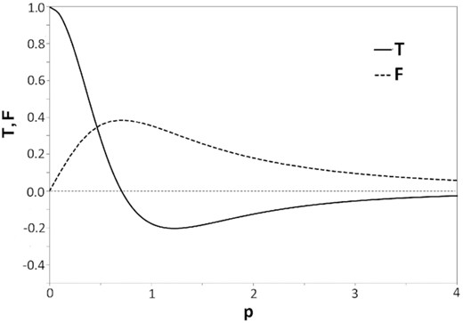
Dimensionless plot of the force function F (dashed curve) and tidal strength function T (solid curve) in a Plummer model for a stellar cluster. The distance variable p is expressed in units of the Plummer radius r0. The units for F and T are |$GM/r_0^2$| and |$GM/r_0^3$|, respectively.
Similar to earlier investigations, we model the solar birth cluster from the very outset, assuming all stars to form momentarily at the same epoch, at which we initialize the cluster and start the dynamical simulation. Our cluster model is initialized using the McLuster software (Küpper et al. 2011) for integration with nbody6++gpu (Wang et al. 2015). This N-body code includes the mass-loss effects of stellar and binary evolution according to the Cambridge stellar evolution package (Hurley, Pols & Tout 2000), which means that both impulsive mass loss by supernova (SN) explosions and continuous mass loss through the winds characterizing the late stages of massive stars are accounted for.

The cumulative distribution function of initial stellar masses (m, in units of M⊙) according to Kroupa (2001).
The McLuster software allows us to specify the binary fraction fbin, i.e. the fraction of all individual cluster stars that are initialized as binary components, as a model parameter. The semimajor axes of binaries are chosen on the basis of Kroupa’s period distribution (Kroupa 1995, 2008). The orbital eccentricities are found by the McLuster default procedure, using a thermal distribution with frequency function f(e) = 2e. Stars with masses |$M \gt 5 \, \mathrm{M}_\odot$| are paired separately from the lower mass stars such that the binary components are either two high-mass or two low-mass stars. The pairing is random within each of the two mass ranges. Our simulations keep track of the dissolution and formation of binaries during the evolution of the clusters. We included the binaries because the option was available and makes the model more realistic, but we note that Adams et al. (2006) and Brasser et al. (2006) found the inclusion or exclusion of binary encounters to play very little role in the dynamics of the young Solar system, and hence they were not included in B12.
Our scheme for primordial mass segregation differs from the method used in B12. We apply the scheme installed in the McLuster code, which uses the method introduced by Baumgardt, De Marchi & Kroupa (2008). This leaves the wanted Plummer structure unchanged. Basically, it introduces a correlation between stellar mass and specific orbital energy, which can be tuned between the extreme cases of 0 per cent and 100 per cent by means of a model parameter s chosen on the interval [0,1].
The initialization of the cluster also involves the gas component. This is assumed to have the density function of a Plummer sphere with the predefined Plummer radius r0, so that the above equations for U, F, and T are accurately satisfied. For the stellar component, in principle, the Plummer density function is mimicked by assigning random, initial radius values to all the stars of different masses using probabilities derived from this common function. However, in reality this is modified by the mentioned mass segregation scheme.
The initial mass Mg of the gas sphere is calculated from the total mass of the stars, M*. If we call ϵ the predefined star formation efficiency, we get Mg = M*(1 − ϵ)/ϵ. The structure of the gas sphere is kept constant, but Mg is treated as a function of time. We use the same formalism as Brinkmann et al. (2017), involving a delay time τd during which Mg remains constant and, directly after this time, an exponential decay with an e-folding time τg. We also follow Brinkmann et al. (2017) in expressing τg as the ratio between the initial half-mass radius of the cluster and a gas expansion velocity of 10 km s−1.
Like in B12, we initialize the stellar velocities so that the virial ratio of the stellar component, i.e. the ratio (Q) between the total kinetic and potential energies, is lower than the equilibrium value of Q = 0.5. This assumption, which is commonly used in recent cluster modelling, is based on observational evidence from very young stellar aggregates. Consequently, the first part of dynamical evolution is a contraction due to the self-gravity of the cluster.
Our treatment of the external, tidal truncation of the cluster differs from that of B12. In our picture, the cluster arises inside a molecular cloud from a high-density core, which with its placental gas forms a self-gravitating, bound entity. This experiences tidal forces from the close environment, which are stronger than those of the Galactic force field. Thus, while B12 considered the far-field picture of the Galactic tides, we treat the near-field tide of a point mass connected to the parental giant molecular cloud (GMC). This may be considered to represent a clump in the turbulent medium, possibly hosting another nascent stellar cluster. We treat it as stationary with a mass of 8000 M⊙ and a distance of |$10\,$|pc. For clusters with 1000 stars and an average stellar mass of 0.573 M⊙ – as relevant for our assumed IMF – the tidal radius expressed as the Hill sphere radius in a circular restricted three-body problem is then somewhat more than 4 pc.
We emphasize that the tidal radius cannot be imposed on our definition of cluster membership. On the other hand, such a definition is needed since the evolution of the cluster involves the escape of many stars to larger and larger distances, while others stay rather close to the initial centre of mass. This phenomenon is a salient feature of cluster evolution in our model due to the efficient route to escape offered by the external, tidal field (Wiśniowski et al. 2021). We have selected a constant limiting distance rlim from the current centre of mass throughout the simulation to define the cluster membership. This centre of mass refers to all the current cluster members, and it is redefined each time a member escapes or returns. We use the current centre-of-mass frame at all times to define the positions and velocities of the members in our analysis of the cluster. This is in fact necessary, since each mass loss from the cluster – be it due to escape beyond rlim or due to stellar evolution – also means a loss of momentum so that the current centre-of-mass frame is in motion with respect to the initial centre-of-mass frame.
This updating, due to the cluster mass loss, might in principle be supplemented by the effects of changes in the GMC structure. However, we consider it beyond our scope to treat those changes realistically and thus we neglect them. In particular, this means that we consider the lifetime of the GMC to exceed the time span of our integrations, which we have specified to 10 Myr. This is supported by observations, which indicate that GMCs typically exist for somewhat longer times (e.g. Gustafsson et al. 2016).
Single stars with masses in the |$[0.95, 1.05]\, \mathrm{M}_\odot$| interval are considered as potential solar templates, meaning that they may represent the Sun in the simulations of planetesimal dynamics. Apart from the stellar mass, no other property is used as a criterion. Hence, contrary to B12, we do not distinguish between initially inward and outward moving stars. Our only orbital bias is the one caused by initial mass segregation, whereby solar mass stars are relatively concentrated toward the cluster centre, belonging to the upper 10 per cent of the IMF. We apply the same limiting distance rlim to the solar templates as for updating the cluster membership. In other words, the effects of the cluster on objects orbiting around the solar templates are taken into account only as long as the stars are cluster members.
2.2 Local features
In our model, we treat the dynamics of the stellar cluster and that of the planetesimal population of a member star separately. Thus, we use the output from the cluster simulation to obtain external perturbations to the planetesimal motions. This is done by applying a standard treatment of many body system dynamics (e.g. Binney & Tremaine 1987), whereby the gravitational potential is separated into two parts: one smooth, global function of position, and one part representing the local potential wells of individual stars. We thus consider the tidal force due to the entire cluster and the close encounters with cluster stars as separate contributors to the external perturbations.
2.2.1 Tidal force
The initialization of our clusters is done so that the stellar mass distribution over radial distance simulates that of a Plummer sphere. We can thus expect that it generates a potential function similar to that of equation (1). However, as time proceeds, the stellar component of the cluster evolves dynamically. As mentioned above, the first principal feature of this evolution is a trend toward virialization. This starts by contraction, caused by the subvirial kinetic energies, which would in principle be followed by a damped sequence of expansions and contractions tending toward virial equilibrium. However, a second feature sets in during the early stages of virialization, and this is an expansion caused by the loss of the gas potential. This halts the virialization process and eventually results in the escape of the majority of the cluster stars. There might also be signs of collisional relaxation in the central parts even during the short time-scale under consideration due to very high stellar densities.
The procedure used is as follows. Consider a certain output from the cluster simulation. We register the distances and masses of all the members of the cluster (i.e. stars with r < rlim). A spatial smoothing is applied such that each star is subject to a radial offset. This is a random length added to the real distance, obeying a Gaussian distribution with zero mean and a predefined standard deviation chosen to represent the statistical uncertainty of the position of any single star as a realization of the underlying density function.2 We also use a temporal smoothing such that we build a pool of entries from 200 consecutive outputs consisting of the individual stellar masses divided by 200 and their offset distances. This pool represents a smoothed, averaged mass distribution during the specific interval of 200 outputs under consideration. The pool is divided into 20 parts with equal numbers of entries such that each part covers its own range of distances. These ranges define a set of consecutive, spherical shells around the cluster centre. The borders defining the shell volumes are placed at the distances of the outermost entries of the inner shells.
The mean density of the shell, i.e. its mass divided by its volume, is associated with the mass-weighted distance of all the contributing entries. From the entire pool we thus obtain 20 couples of density and distance values, which in principle serve as the basis for the fit of polynomial coefficients. The exception is the innermost shell, for which we need better spatial resolution and therefore split it into eight parts in the same way as done for the 20 shells. Thus, overall, we get 27 couples for the least-squares fit.
Fig. 3 illustrates the fit of the density function for two cases, calculated from cluster outputs centred at |$t = 1\,$|Myr. As seen, the data to be fitted are sometimes rather noisy in spite of our smoothing procedures. Fundamentally, this reflects the presence of strong, local mass concentrations in the form of massive stars or binaries.

Illustration of the polynomial fits for the density function in two cluster models at a cluster age of |$1\,$|Myr. The red dots show the values of mean density in 27 concentric shells, and the solid curves show the sixth-degree polynomial fits. Note that the scatter of the data points is much larger for cluster A1 than for cluster B1.
We emphasize that the analytic function ρ*(r) is supposed to represent a parent mass distribution, which is sampled by the simulated stellar distances through the above-described pool. This calls for a discussion of the sampling uncertainties and their possible influence on the fitted function. In particular, the numerical data originate from a certain range of distances, where the pool can be considered reliable, and we wish to avoid extrapolation outside this range. This means extrapolation to distances, where there are no stars. We hence cut the density function outside the distance of the outermost cluster member during the interval of temporal smoothing. On the other hand, special attention has to be paid to the innermost part of the cluster.
Here, the density and tidal force are often very large. However, this does not guarantee the presence of simulated stars extremely close to the centre. The innermost star is often situated at |$r\sim 0.1\!-\!0.2$| pc. The local value of the fitted density function at this point may be much lower than the projected value at the very centre (as given by the a0 coefficient). The full amount of this increase has a statistical uncertainty at least as large as that of a0. However, we have checked the performance of the polynomial fits by comparing the masses within the different shells as found by integration of ρ*(r) to the actual pool masses contained within the shells as a safeguard against unreasonable behaviour of the fitted density function. This comparison did not reveal any problems in the innermost part of the clusters. On the average, the density functions predict a somewhat too small total cluster mass, which we ascribe to the fact that these functions have a positive curvature. Thus, the integrated mass tends to be smaller than the one found by assuming a constant density equal to the one calculated as the average for the shell.
We emphasize that our assumption of a smooth parent distribution is meaningful only as long as N is large. It may be used as a crude approximation even when, strictly speaking, N is somewhat on the small side – however, it should not be used for dissolving clusters near the end of their lives. In this case – specifically, when N < 100 – we do not consider any tidal action of the cluster and only include the effects of intruding stars as described below.
2.2.2 Close encounters
To deal with the close encounters, we use the following method. First, we identify the cluster stars whose planetesimal populations shall be simulated. As noted above, when simulating Oort Cloud or sednoid formation in the Solar system, single stars are considered and solar templates are chosen among such stars with masses close to the solar mass. For each of those stars, we use the cluster simulation outputs to prepare a catalogue of close encounters. To this end, we first define a limiting distance for the selected encounters. The choice made may depend on whether the focus is on sednoids or Oort Cloud comets, but in any case the encounters need to stand out from the normal passages of neighbouring stars in terms of their effects on the planetesimal population. We also need to make sure that the output interval of the cluster simulation is short enough to run a minimal risk of missing an encounter.
The positions of the selected stars are passed to the planetesimal simulation at all output times, when the distance to the template star is less than the limiting encounter distance. The treatment of encounters with binaries is not of prime importance. When dealing with close binaries, the output interval may not resolve the internal motion in the binary. On the other hand, the simple solution of linear interpolation between subsequent output positions for each binary component yields a fair approximation to the true motions.
For binaries, the strength parameter normally refers to the encounter parameters of their internal centre of mass. If this is large enough, both components are selected. However, especially for wide binaries, it may happen that only one component penetrates inside the limiting distance or that both components perform encounters separated in time. If so, we consider the individual S value of each penetrating component to decide about its selection.
3 RESULTS
We shall now present some results of our investigation of four basic cluster models. The dynamical evolution of these models is studied in Wiśniowski et al. (2021). In Table 1, we list the values chosen for the above-mentioned model parameters. Some of these are target values, which means that the initialization aims to reproduce them but that the exact values may differ, depending on the initial random number seed. Hence, while the initial number of stars is always N = 1000, in individual realizations of the cluster model the initial, total stellar mass varies. In addition, the IMF range from about 50 to 100 M⊙ is seriously undersampled. The highest stellar masses in individual realizations may therefore differ a great deal, and consequently also the total stellar masses. This is also reflected in the gas masses, which are strictly linked to the stellar masses by the constant value of ϵ.
Physical parameters characterizing our initial cluster models. The values of r0 and τg are strictly related, while those of τd are independent.
| Parameter | Notation | Values |
|---|---|---|
| Number of stars | N | 1000 |
| Star formation efficiency | ϵ | 0.33 |
| Plummer radius (pc) | r0 | 0.585, 1.17 |
| Gas expulsion delay (Myr) | τd | 0.6, 2.4 |
| Gas expulsion e-folding time (Myr) | τg | 0.077, 0.153 |
| Virial ratio (target) | Q | 0.15 |
| Binary fraction | fbin | 0.3 |
| Mass segregation strength | s | 0.5 |
The four cluster models form a grid defined by two different values of the Plummer radius and two different values of the delay time for gas dispersal. In each of these cases we have performed three simulations with different random number seeds, thus obtaining three realizations of each model. We denote the cluster models by capital letters A, B, C, and D, where A and B have the larger Plummer radius, and A and C have the shorter delay time. Whenever necessary, individual realizations are identified by digits 1, 2, and 3.
3.1 Density and force fields
In the four panels of Fig. 4, we present stellar density functions for four cluster models calculated at a given set of times in the cluster evolutions, each one situated in the middle of its respective sampling interval. For comparison, a dashed curve is added to show the initial Plummer function in each plot.
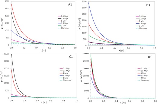
Density functions fitted at different evolutionary times (see legends) for four cluster model realizations. The panels refer to models A (upper left), B (upper right), C (lower left), and D (lower right). The density variation of the initial Plummer model is shown by a dashed curve.
We emphasize that the plotted density functions represent the results of dynamical evolution, and it is well known that the dynamics of ∼1000-body systems like our clusters is extremely chaotic. Thus, we cannot expect the results for three random realizations of a given cluster model to be very similar to each other. Indeed, we sometimes see similarities and sometimes striking differences. The reader should be cautioned against interpreting the density curves of Fig. 4 as representing some general truth about the models in question – in fact, they only represent the respective realizations.
Nevertheless, it is our impression that, even though vague and tentative, some conclusions are warranted as to the role that the cluster model plays in affecting the outcome. The realizations shown by the plots in Fig. 4 have been selected to illustrate these conclusions. The first observation is that the more strongly concentrated models C and D reach much higher central densities than models A and B.
For models A and B, the central stellar density of the initial Plummer model is about |$100\, \mathrm{M}_\odot $| pc−3. The maximum values observed are mostly about 30 times higher, and this compression is due to the fact that the clusters contract to establish virial equilibrium. We note a trend for a time shift such that these values occur after |$1\,$|Myr for model A and |$1.5\,$|Myr for model B. This indicates that the peak values in model A are somewhat damped by the early loss of the gas at |$0.6\,$|Myr, which tends to halt the contraction.
For models C and D, the central stellar density of the initial Plummer model is about |$800\, \mathrm{M}_\odot $| pc−3. This is now amplified by factors of about 30–70 due to the initial contraction. For model C, the plot in Fig. 4 indicates a highest central density of about |$3 \times 10^4\, \mathrm{M}_\odot $| pc−3 occurring after only |$0.5\,$|Myr of evolution. The actual maximum of the central density is likely even higher and occurs somewhat earlier or later. In the present case we checked this and found the maximal value of |$3.8 \times 10^4\, \mathrm{M}_\odot $| pc−3 to occur after |$0.44\,$|Myr. Like in the case of models A and B, we notice a time shift of the maximal densities such that these occur after 1.5 or |$2\,$|Myr in model D. Again, this suggests that the maximal densities of model C may be damped by the early gas loss.

Tidal strength versus distance at different evolutionary times (see legends) for the same four cluster model realizations as in Fig. 4.
3.2 Encounter statistics
As limiting value for the minimum distance of close encounters we have chosen |$40\,$|kau. Among all the potential solar template stars of each cluster simulation we have randomly selected six for use in the simulations of planetesimal dynamics. We have recorded the total number of stellar intruders in each case and the number of selected intruders according to the above-mentioned criteria. For the energy criterion we require the kinetic energy of the intruder at the moment of closest approach to be no larger than four times the binding energy of the system formed with the solar template. For the strength criterion we measure S in units of |$\, \mathrm{M}_\odot$| for the masses, km s−1 for the velocities, and kau for the encounter distances, and we require the dimensionless value of S to exceed 0.04 for selection. Here we will present some relevant statistics of the resulting numbers of selected close encounters.
In Table 2, we show the relevant total numbers of intruders and the numbers of selected ones for all the 12 simulated clusters. A striking feature is that the total numbers of encounters per template star separate into four groups corresponding to the four basic models. Primarily, models C and D have by far the largest numbers when compared to models A and B, respectively, showing a strong influence by the degree of initial concentration. Moreover, comparing models with equal concentration, models B and D dominate over models A and C, respectively, showing an influence by the delay time of gas expulsion.
Total number of encounters within |$40\,$|kau (Ntot) for the six chosen solar templates, number of encounters selected according to the energy criterion (NE), number of additional encounters selected according to the strength criterion (NS), and fraction of selected encounters (fsel) among the total for each cluster simulation.
| Simul. | Ntot | NE | NS | fsel |
|---|---|---|---|---|
| A1 | 228 | 20 | 20 | 0.175 |
| A2 | 242 | 5 | 19 | 0.099 |
| A3 | 205 | 9 | 19 | 0.137 |
| B1 | 381 | 16 | 27 | 0.113 |
| B2 | 426 | 18 | 24 | 0.099 |
| B3 | 773 | 25 | 31 | 0.072 |
| C1 | 915 | 21 | 71 | 0.101 |
| C2 | 1045 | 19 | 54 | 0.070 |
| C3 | 1148 | 12 | 65 | 0.067 |
| D1 | 2074 | 21 | 74 | 0.046 |
| D2 | 2045 | 33 | 113 | 0.071 |
| D3 | 2067 | 25 | 99 | 0.060 |
We also note that most of the selected encounters have S > 0.04 and are thus selected on this criterion. However, an important fraction is instead selected on the energy criterion independent of the S values. In this respect, in the A and B models a larger fraction is energy selected than in models C and D. This also holds for the selected fraction at large.
The statistics of total numbers of encounters can be understood on the basis of the plots in Fig. 4, if we interpret the plotted stellar mass densities as indications of the stellar number densities. Mass densities in excess of |$1000\, \mathrm{M}_\odot \,$|pc−3 correspond to number densities of |${\sim} 2000\,$|pc−3 or more, yielding a very high encounter rate (see Proszkow & Adams 2009). Such conditions occur in all the models though covering larger distance intervals and lasting for longer times and reaching higher levels in clusters with stronger concentration or more delayed gas loss.
Fig. 6 shows a histogram of the total number of intruders per solar template star for all the 72 solar templates associated with the 12 simulations. The template stars have been coloured differently for the low- and high-concentration models, and the difference between these two groups stands out clearly. More than 150 intruders per template is rare for the low-concentration models but is rather the rule for the high-concentration models. Moreover, it can be seen that the scatter of the number of encounters is significantly larger for the individual templates than for the different simulations. Thus, the number of encounters experienced by any particular star depends more on the orbital evolution of that star than on the corresponding cluster evolution.

Distribution of the number of stellar intruders encountering each solar template star to within |$40\,$|kau for all the 12 cluster simulations. The less concentrated A and B clusters are plotted in red, and the C and D clusters are plotted in blue. On top of the histogram, the numbers averaged over the six chosen templates of each individual simulation are indicated.
In Fig. 7, we show the distribution of distance from the cluster centre versus time for all the selected encounters, separately for the two cluster types with different degrees of concentration. The stronger concentration to small distances in panel (b) follows from the smaller distances at large in models C and D, and this is especially accentuated at early times because of the fact that, as a consequence, the time-scale for initial contraction is shorter. A large majority of encounters occur within ∼1.5 pc in models A and B, and within ∼0.75 pc in models C and D. A conspicuous dearth of encounters after about 3–4 Myr is obvious in both panels due to the waning of the central density peak. This dearth only concerns distances less than about 1–1.5 pc.

Distance from the cluster centre versus time for the selected encounters. Panel (a) shows results for the A and B models, and panel (b) represents the C and D models.
4 DISCUSSION AND CONCLUSIONS
In this work, we have introduced a new model to describe the dynamical effects due to the presence of a stellar birth aggregate on a population of planetesimals undergoing gravitational scattering by giant planets around one member of the aggregate. Our current aim is to study the formation of very distant small body populations around solar-type stars as exemplified in the Solar system by the Oort Cloud and the sednoids. However, the model may just as well be used in studies of planetary system evolution or planet formation in extended protoplanetary discs. It combines the development of numerical models of embedded clusters by N-body simulations with the use of these models to provide the action of the clusters in the vicinity of solar-type member stars through a smooth tidal force and close stellar encounters.
We stress two features that distinguish our model from those that have been used previously by other authors. The external perturbations to the planetesimal orbits are modelled using a combination of a smooth, tidal gravity field representing the whole aggregate, evolving with time as the aggregate evolves dynamically, and a selection of close encounters by single or binary stars expected to impart the strongest impulses to the solar template star and its orbiting planetesimals. The other feature is that the dynamical evolution of the aggregate is modelled by including the tidal interaction with a relatively nearby, massive clump in the surrounding GMC, which allows for an efficient escape route of stars from the considered aggregate.
The first item to discuss is the classical separation of the ambient potential into the smooth and slowly evolving background field of the aggregate as a whole and a fluctuating component due to passages through the potential wells of single stars or binaries. In principle, one problem is that the encountering stars are treated twice during the encounters, since they also form part of the entire aggregate whose gravity is simulated by the tidal field. The alternative of defining a time interval, when the encounter occurs, during which the tidal field is recomputed for the decimated aggregate without the encountering stars suffers from the artificial jumps of the tidal field at the beginning and end of the interval. Compared to this, we find it better to neglect the slight perturbation of the tidal field caused by the presence of the unwanted stars.
Of more concern is the choice of the limiting distance for the close encounters. It is obvious that the selected encounters have to stand out by a wide margin from the ever present, distant encounters that mostly have negligible effects. The simple way to guarantee this is to choose a small value for the maximum distance of the considered encounters. However, this has to be weighed against the size of the extracted population. For sednoids with semimajor axes less than |$1000\,$|au, it is reasonable to limit the encounter distances to less than |$10\,$|kau, but when the inner core of the Oort Cloud is considered with semimajor axes of several kau, more distant encounters are likely of importance as well.
In the latter case, the distinction of the selected encounters from the rest becomes less clear, and we have no guarantee that the selection actually made will be optimal. We have to admit that this problem may have some influence on the simulation results for Oort Cloud formation. However, it is difficult to imagine that these results could be seriously inaccurate. Moreover, we have taken all reasonable measures to reduce the problem. An overarching principle is to rather include some encounters with negligible effects than exclude some that are relatively important.
For instance, the rare events where the solar template is temporarily captured into a binary with the intruding star may obviously lead to important effects. However, these are essentially unpredictable, and our decision is to include all of them. The same goes for very slow encounters without gravitational binding, where the excess energy of motion is not much larger than the binding energy. In the remaining cases we judge the strength parameter S to be a rather reliable indicator of the expected importance of a given encounter.
Concerning the cluster evolution, we have modelled a small selection of cases with 1000 stars initially in a Plummer density distribution with about 0.5 or |$1\,$|pc radius. No substructures have been considered. Because of the subvirial velocities of the stellar initial conditions, the aggregates at first evolve by a contraction, which is quite prominent even for a gas escape time as short as |$0.6\,$|Myr. This sets up a cuspy density profile, where the central value tends to be at least ∼30 times higher than for the initial Plummer distribution. In connection with this, the strength of the tidal gravity field reaches significant values for distances less than |${\sim} 0.2\!-\!0.3\,$|pc from the centre. In the more concentrated models, this feature may persist for several Myr.
Hence, only template stars penetrating inside this region will experience strong enough cluster tides to likely contribute to the angular momentum transfer under consideration. A similar situation holds for the close encounters, because the stellar number density is very small at larger distances. We defer further discussion of this to our future papers, where the perihelion extraction process will be simulated.
As discussed in Wiśniowski et al. (2021), the presence of the nearby clump and its tidal field is a main reason for the rapid dispersal of our stellar aggregates. This feature is in broad agreement with observations and is sometimes referred to as ‘infant mortality’. However, some star clusters obviously manage to survive for times of |${\sim} 100\,$|Myr or more, as shown by the Galactic open clusters. It is of obvious interest to study the formation of sednoid or Oort Cloud formation in such scenarios as well, but our present sample of aggregates is too small to present any such survivors.
In conclusion, our modelling of embedded cluster evolution and circumstellar dynamics around solar template stars inside such clusters represents a new level of ambition, as compared with all previous investigations. This allows us to gain new insights into the roles of cluster tide and close encounters in the perihelion extraction process affecting distant planetesimals. These, in turn, will be very helpful when interpreting the results of forthcoming simulations of such extraction and understanding the formation of the sednoid and Oort Cloud populations. As our discussion has shown, there is a price to pay for such an advance, consisting of some principal problems with the separation of global and local cluster effects. To some extent, this compromises the performance of the current version of our model.
ACKNOWLEDGEMENTS
We gratefully acknowledge clarifying discussions with Mirek Giersz during the planning of this work, and helpful advice on running the nbody code by Wang Long. We are also grateful for the advice of anonymous referee, which led to a major improvement of the paper.
DATA AVAILABILITY
Data available on request.
Footnotes
This term usually stands for semimajor axes |${\lt} 10\, 000\,$|au and is different from the Inner Oort Cloud.
We use a Gaussian, cut at ±3σ, with a maximum value of |$0.25\,$|pc for σ.
