


ABSTRACT
The electromagnetic counterparts to gravitational wave (GW) merger events are highly sought after, but difficult to find owing to large localization regions. In this study, we present a strategy to search for compact object merger radio counterparts in wide-field data collected by the Low-Frequency Array (LOFAR). In particular, we use multi-epoch LOFAR observations centred at 144 MHz spanning roughly 300 deg2 at optimum sensitivity of a since retracted neutron star–black hole merger candidate detected during O2, the second Advanced Ligo–Virgo GW observing run. The minimum sensitivity of the entire (overlapping) 1809 deg2 field searched is 50 mJy and the false negative rate is 0.1 per cent above 200 mJy. We do not find any transients and thus place an upper limit at 95 per cent confidence of 0.02 transients per square degree above 20 mJy on one, two, and three month time-scales, which are the most sensitive limits available to date. Finally, we discuss the prospects of observing GW events with LOFAR in the upcoming GW observing run and show that a single multibeam LOFAR observation can probe the full projected median localization area of binary neutron star mergers down to a median sensitivity of at least 8 mJy.
1 INTRODUCTION
The landmark detection of gravitational waves (GWs) from binary neutron star (BNS) merger GW170817 (Abbott et al. 2017a) and of its electromagnetic (EM) counterpart spanning the full spectrum has taken us fully into the era of multimessenger astronomy (Abbott et al. 2017c). The rich observational data set of this single event proved to be a trove of scientific breakthroughs affecting many aspects of astronomy (e.g. Abbott et al. 2017b; Cowperthwaite et al. 2017; Margalit & Metzger 2017). Given the unparalleled impact from the extensive multiwavelength follow-up campaign of GW170817, there is wide interest in pursuing the EM counterparts of other GW merger events involving at least one neutron star, and particularly of a black hole and neutron star (BH–NS) for the first time (e.g. Coughlin et al. 2019; Dobie et al. 2019; Andreoni et al. 2020; Antier et al. 2020; Page et al. 2020; Alexander et al. 2021; Boersma et al. 2021). However, this endeavour comes with substantial challenges, due in large part to the significant uncertainties on the location of GW events: the median 90 per cent credible region of the sky localization area in the previous Advanced Ligo–Virgo GW observing run (O3) was approximately 200 deg2 (Abbott et al. 2020). While event localization improves with each subsequent GW observing run, large survey speeds and telescopes with large fields of view in particular will remain instrumental in efforts to identify GW EM counterparts in the upcoming observing run (O4), which is likely to commence in the latter half of 2022.
Radio interferometers are particularly promising tools for identifying the exact location of a GW event, owing to their combined large fields of view and sensitivity, as well as low-latency observing capability. The interaction of the relativistic jet that is launched in the moments following a BNS (and possibly BH–NS) merger with the circum-merger medium produces a radio afterglow that is detectable days to weeks post-merger at GHz frequencies and lasting months to years (Paczynski & Rhoads 1993; Mészáros & Rees 1997). This emission was studied at unprecedented detail with radio observations of GW170817 (Abbott et al. 2017c; Hallinan et al. 2017). This synchrotron emission contains key information about the enigmatic jet that produced it and can be traced across the radio band as it evolves dynamically (Alexander et al. 2017, 2018; Corsi et al. 2018; Dobie et al. 2018; Margutti et al. 2018; Mooley et al. 2018a, b, c; Resmi et al. 2018; Troja et al. 2018; Ghirlanda et al. 2019; Hajela et al. 2019). In addition to afterglow emission from a relativistic jet, a second synchrotron afterglow component caused by the dynamical/kilonova merger ejecta is predicted to dominate the radio light curve and to peak at low radio frequencies years following the merger (Nakar & Piran 2011; Hotokezaka et al. 2016). This never-before-seen radio afterglow would contain important information regarding the merger ejecta, which, for instance, can be used to make inferences about the elusive equation of state of nuclear matter. Apart from incoherent later-time radio emission, coherent emission produced around the merger time has long been predicted by various mechanisms (e.g. Usov & Katz 2000; Hansen & Lyutikov 2001; Pshirkov & Postnov 2010; Piro 2012). In particular, it has been suggested that a fraction of fast radio bursts (FRBs) could be accounted for by prompt emission arising from the coalescence of compact objects (e.g. Totani 2013; Falcke & Rezzolla 2014; D’Orazio et al. 2016). Low-latency triggered radio observations covering the localization region of GW merger events would enable us to directly test these theories (Chu et al. 2016; Rowlinson & Anderson 2019; Gourdji et al. 2020).
The Low-Frequency Array (LOFAR; van Haarlem et al. 2013) has been used with its large field of view to follow-up on GW events at 145 MHz since the first LIGO/Virgo observing run (Broderick et al. 2015a, b; Abbott et al. 2016; Broderick et al. 2017; Rowlinson et al. 2017a, b). In particular, the location of GW170817 was observed on several epochs, the results of which are reported in Abbott et al. (2017c) and Broderick et al. (2020). The event’s low elevation relative to LOFAR greatly affected the sensitivity achievable and thus the ability to place constraints on the radio light curve at low radio frequencies. LOFAR late-time follow-up results from the third GW observing run will be reported by Gourdji et al. (in preparation).
In this paper, we present our strategy to search for GW merger radio afterglows in wide-field LOFAR data. We use wide-field multi-epoch LOFAR observations of G299232, a since ruled-out BH–NS GW trigger from the second GW observing run (O2), to establish and demonstrate our observing, calibration and transient search strategy, to guide future LOFAR follow-up of GW triggers and to examine the background of unrelated transient events. In Section 2, we describe our observations, data calibration, and imaging. In Section 3, we outline the three transient search methods undertaken. Our results are presented and discussed in Section 4. We discuss the prospects for LOFAR observations during the upcoming GW observing run in Section 5 and conclude in Section 6.
2 OBSERVATIONS AND DATA REDUCTION
2.1 Observations
The data presented in this paper come from LOFAR follow-up observations of G299232 (also known as GW170825), a GW BH–NS merger candidate detected on 2017 August 25 at 13:13:37 ut during O2 and originally classified as EM-bright (LIGO Scientific Collaboration/Virgo Collaboration 2017). The candidate was not detected in offline analysis by the LIGO/Virgo collaboration published 2 yr later (Abbott et al. 2019). The 50 and 90 per cent confidence intervals of the sky localization area were 451 and 2040 deg2, respectively. The GW location probability skymap and LOFAR coverage are depicted in Fig. 1. To probe the large localization region of the candidate event, we tiled 47 unique LOFAR beams each with a full width at half-maximum (FWHM) of 3.8° and using a beam spacing of around 2.8° (approximately equivalent to the beam FWHM divided by |$\sqrt{2}$|) to enclose 289.4 deg2 of the localization region within beam radii of 1.4° (blue circles in Fig. 1), but with further coverage at the outer edges of the beam pattern (we search out to beam radii of 3.5°, represented by the dashed blue line in Fig. 1). We henceforth refer to the area of sky covered by a single LOFAR beam as a ‘sub-field’. Each sub-field was observed for 225 min at 3 epochs corresponding to roughly 1 week, 1 month, and 3 months following the GW trigger, as described in Table B1. A total of 48 LOFAR beams were used, but two were centred on the position of a neutrino candidate (Bartos et al. 2017a, b) to provide an opportunity to stack the data and potentially improve sensitivity, leaving 47 unique sub-fields. The data were collected using LOFAR’s HBA Dutch stations (24 core stations and 14 remote stations) in the HBA_DUAL_INNER configuration. Per epoch, we performed four 8-h observing runs using two pointings. To optimize the u-v coverage, we alternated between two pointings every 25 min during each 8-h observing run. Each pointing direction was comprised of six beams centred at 144 MHz. Each beam, in turn, consisted of 81 frequency sub-bands with a bandwidth of 195.312 kHz, yielding a total beam bandwidth of 15.82 MHz. Each observation was book-ended by a 10 min calibrator scan of 3C 48 and 3C 196, in that order. The data were recorded using 2-s integration time-steps and 64 channels per sub-band.
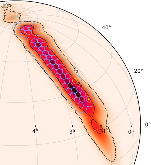
Part of the three-detector GW location probability density map of G299232 (LIGO Scientific Collaboration/Virgo Collaboration 2017). Contours enclose 50 and 90 per cent of the probability density (though additional regions in the Southern hemisphere are not included here). The full extent of the area searched in this analysis is enclosed by the blue dashed line, and corresponds to 47 overlapping LOFAR beams each searched out to a radius of 3.5°. The blue circles denote beam coverage of radius 1.4°, and the resulting unique sky area covered by these radii is 289.4 deg2. The optical transient detected contemporaneously with the GW trigger is shown by a yellow dot. The LOFAR beam placed at the centre of the neutrino candidate uncertainty region is shown in yellow. All beams are spaced by 2.8°, except for the two beams that were centred on the respective locations of the optical transient and the neutrino candidate. This figure was created using the ligo.skymap python module.1
2.2 Calibration and imaging
Immediately following the observations, both the calibrator and target data were averaged in time and frequency to 10 s and 48.82 kHz (4 channels per sub-band) during pre-processing to reduce data volume and Cas A was subtracted from the visibilities using the so-called demixing procedure due to its close proximity. Standard LOFAR RFI flagging was also carried out during pre-processing, as described in Offringa, van de Gronde & Roerdink (2012).
The interferometric data were calibrated using prefactor,2 a pipeline developed to correct for instrumental and ionospheric effects present in LOFAR data sets (de Gasperin et al. 2019). The prefactor calibration process begins by comparing observations of a calibrator source to the LOFAR skymodel of the calibrator source. This step provides direction-independent gain corrections that can be applied to the target observations. Once the target data are calibrated, they are imaged using the full bandwidth via WSclean3 (Offringa et al. 2014), which is the final data product used for our scientific analysis.
We used 3C 196 to calibrate our data using the Pandey flux density model (which is consistent with the Scaife & Heald model; Pandey & Lofar Eor Group 2014), except for observations taken on 2017 August 31, where station data were missing and so the back-up calibrator scans of 3C 48 (Scaife & Heald 2012 flux density model) were used instead. The sub-bands comprising each beam were concatenated into three groups of 27 sub-bands, each with a total bandwidth of 5.273 MHz. The gain solutions from the calibrator were then applied to the target data. Sky models from the 147.5-MHz TIFR Giant Metrewave Radio Telescope Sky Survey First Alternative Data Release (TGSS; Intema et al. 2017) were used for direction-independent phase corrections for our target observations.
The resulting calibrated data were used as input for WSclean to create image products. These include a primary-beam corrected image covering the full 15.82 MHz observing bandwidth to be used for analysis, as well as individual images of the three groups of sub-bands (centred at 139 MHZ, 144 MHz, and 150 MHz each with bandwidths of 5.273 MHz) for reference purposes should a transient candidate appear in the full-bandwidth image. The WSClean options were optimally chosen for point sources and we used Briggs weighting with robustness parameter 0.5. We used baselines out to a maximum length of approximately 16 km. The resulting images have a pixel resolution of 5 arcsec to sample the restoring beam of our images (2D Gaussian fit of the image point spread function), which on average has a major axis of 26.5 arcsec and minor axis of 18.2 arcsec.
We checked the flux density scale of our data by comparing to the TGSS catalogue (Fig. 2), as described in Section 3.1.2. We fit the data using orthogonal distance regression, which takes into account the uncertainties in both catalogues’ source fluxes. We considered bright and compact matched sources with integrated flux density measurements in excess of 1 Jy beam−1 in the TGSS catalogue. For this, we used only those sources that were fit by a single Gaussian in the TGSS catalogue and that have an integrated flux to peak flux ratio less than 1.3 (the origin of this value is discussed in Section 3.1.2). Sources that are compact in the TGSS catalogue should generally be compact in our TraP catalogue as the major axis of the PSFs are comparable. We find TGSS source flux measurements to have an average offset of 0.8 per cent. We attribute this negligible offset to the different flux models used (TGSS uses Scaife & Heald 2012) and possibly direction-dependent flux scale variations. For reference, we include a flux scale comparison using all compact TGSS sources above the 200 mJy completeness threshold, in the top panel of Fig. 2.
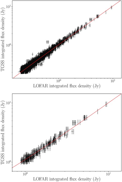
Comparison of source flux densities measured by TGSS and by TraP for the LOFAR data. Only compact sources with integrated flux densities exceeding 200 mJy (top panel) and 1 Jy (bottom panel) are considered. The fits were obtained via orthogonal distance regression and find a TGSS to TraP flux density ratio of 1.04 (top) and 0.99 (bottom). The TraP error bars correspond to the 1σ uncertainties on integrated source flux density values, and the TGSS error bars correspond to the same 1σ uncertainty plus an additional fractional error of 10 per cent, as reported in the TGSS catalogue.
3 TRANSIENT SEARCH
For each individual sub-field, we process the set of three full-bandwidth images (one image per epoch) through the LOFAR transients pipeline (TraP, Swinbank et al. 2015), which identifies and extracts sources detected above 7σ in each image in a 3.5° radius from the beam centre. TraP identifies common sources between images and, if a source that is extracted in the second or third image is not matched to a source from an earlier image, it is flagged as a new source.
We conduct three types of GW transient searches. In the first (Section 3.1), we compare the catalogue of TraP sources found in our images to the TGSS catalogue that spatially overlaps. We compare to TGSS rather than to the LOFAR Two-metre Sky Survey (LoTSS; Shimwell et al. 2019) as only a fraction of our field has been covered by LoTSS to date. This comparison serves additional functions apart from a general GW counterpart search: it allows us to verify the quality and flux scale of our catalogue, derive a transient false-alarm rate, and establish transient search criteria while retaining completeness. The second GW transient search (Section 3.2) goes deeper in sensitivity and consists of comparing the TraP sources found between epochs and investigating potential new sources. The third search (Section 3.3) consists of targeted searches at the location of potential GW-related transient candidates detected at other wavelengths.
3.1 Comparison to TGSS
3.1.1 Catalogue properties
The TGSS survey and our data have comparable resolutions. The TGSS survey uses a 25 arcsec circular restoring beam for the declinations observed in this study. We note that the emission we are targeting would appear as an unresolved point source in our data. First and foremost, we account for TGSS’s lower sensitivity. TGSS is 100 per cent complete above a flux of 200 mJy. The detection threshold used for TGSS is 7σ, where σ is the local noise, the median of which is 3.5 mJy beam−1 (Intema et al. 2017). Therefore, the median sensitivity of the survey is 24.5 mJy. For comparison, the median local rms and sensitivity (7σ) of our LOFAR data is 1.7 and 12.0 mJy, respectively, with 80 per cent of our data having a sensitivity below 16 mJy (see Fig. 3). To account for differences in sensitivity between images as well as the decrease in sensitivity from the beam centre of a given image, we calculate the average rms σμ in four annuli of equal area for each image. We divide the entire range of fluxes Fν of all the sources blindly detected by TraP into N bins and weight the number of sources found in each bin by the total fractional area where the condition Fν > 7σμ is met. This allows us to construct a true log(N)-log(Fν) source count distribution and compare the probability of source detection in our data (Fig. 3). The results are tabulated in Table B2. The worst 7σ sensitivity of the complete data set is 50 mJy.
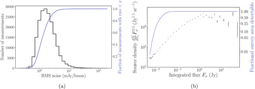
Left: distribution of nearly 200 000 rms noise measurements taken across 141 LOFAR images. The blue curve represents the cumulative distribution of rms noise measurements. Right: Euclidean-normalized differential source density, with counts weighted by the fractional survey area detectable to correct for varying sensitivity between images as well as within a single image (as a function of distance from beam centre). All counts are normalized by the total survey area to obtain source density values. Error bars correspond to the propagated Poissonian error on each count. The data are tabulated in Table B2. The blue curve represents the inverse of the weights given in Table B2 and corresponds to the fractional survey area in which a source with flux Fν is detectable.
3.1.2 Catalogue comparison and transient search
After setting a lower flux cut of 200 mJy, we remove spurious TraP source detections caused by correlated noise or artefacts from sidelobes around bright sources (see Fig. A1). These can be identified rather easily as they are not expected to be consistently extracted in all epochs and typically have large positional uncertainties. We filter out spurious sources by excluding non-persistent sources (i.e. those not detected in all three LOFAR images) with positional error radii greater than 1 arcsec. The value was determined heuristically during the catalogue comparison described below.
There are two aspects that challenge a direct catalogue comparison. The first has to do with the different ways in which complex sources are extracted and modelled. TGSS models complex sources using multiple Gaussian fits, whereas TraP models all sources using a single Gaussian, and does not distinguish overlapping sources. Thus, comparing the catalogues directly will lead to false TGSS transients as, for a given complex source or cluster of sources, there will be multiple unique TGSS sources catalogued but only one TraP source. Given that the transients we are targeting will be unresolved point sources, we include only those TGSS sources that were fit with a single Gaussian (labelled ‘S’ in the TGSS catalogue).
The second challenge is distinguishing between resolved and unresolved sources consistently between catalogues. While an unresolved point source should theoretically have a ratio between integrated flux and peak flux (|$\frac{F_{\rm {tot}}}{ F_{\rm {peak}}}$|) equal to one and source size fit equal to the restoring beam, this is often not the case due to imperfect calibration and finite visibility sampling. These effects naturally differ between catalogues resulting in different degrees of smearing, which causes this ratio (|$\frac{F_{\rm {tot}}}{ F_{\rm {peak}}}$|, henceforth referred to as the ‘compactness’) to be greater than one for a given source. Furthermore, the amount of smearing is strongly dependent on the signal-to-noise ratio (S/N). Thus, a universal cut on compactness is not possible a priori. Fortunately, Intema et al. (2017) provide an empirical distinction between resolved and unresolved sources as a function of S/N in the TGSS catalogue. We use fig. 11 from Intema et al. (2017) to conservatively choose a large value that encompasses all unresolved sources above 200 mJy (|$\frac{F_{\rm {tot}}}{F_{\rm {peak}}}\lt 1.3$|). This leaves 3936 (not all unique) TGSS sources to match to our TraP catalogue. As we do not yet know what the corresponding compactness threshold is in our data, we first look for matches to this subset of TGSS sources in our TraP catalogue (the mean source property values are used for unique sources that are detected across multiple LOFAR epochs), which we limit to sources with |$\frac{F_{\rm {tot}}}{ F_{\rm {peak}}}\lt 5$| and |$F_{\rm {tot}}\gt 200$| mJy as a first pass. This results in 8572 (not all unique) TraP sources to match from. A small fraction of TGSS sources with |$F_{\rm {tot}}$| slightly greater than 200 mJy will be unmatched if their TraP counterpart has |$F_{\rm {tot}}$| slightly less than this cut. There are 197 such cases and matches are recovered by searching below the lower flux cut. Five TGSS sources remain unassociated.
We then proceed to look for unresolved TraP sources without a counterpart in the TGSS catalogue, as these would be transient candidates. To determine a boundary between unresolved and resolved sources in our data above 200 mJy, we take the maximum value in the distribution of compactness values of the TraP matches. This process is done for each sub-field, as the compactness boundary between resolved and unresolved sources varies between sub-fields (the mean compactness boundary is 1.7, with the largest value at 2.3). These cuts are very conservative given that the set of TGSS sources matched from is certain to contain some resolved sources, and so likewise our derived set of TraP unresolved sources is certain to include some resolved sources. We are left with 2324 unmatched TraP sources after applying this compactness filter.
A TGSS counterpart is not immediately found for a significant fraction of these TraP sources because, for reasons not entirely clear, some compact sources are classified as complex sources (i.e. not type ‘S’) in the TGSS catalogue. This likely has to do with subtleties in the source extraction step and we note that TraP uses a different source extraction tool (PySE; Carbone et al. 2018) than is used for TGSS (PyBDSF; Mohan & Rafferty 2015). Therefore, for the remaining unmatched sources, we search for counterparts in the full catalogue of TGSS sources (that is, allowing all fit-types, not only single-Gaussian sources and no compactness or lower flux cuts) and successfully find counterparts. TGSS matches are found for all 2324 remaining TraP sources.
3.2 Deep blind transient search
The sensitivity of the previous transient search is limited by the completeness of the TGSS catalogue. In order to go deeper, we look for transient sources between our images. Low-frequency radio waves from a GW afterglow caused by a jet are expected to be visible on month time-scales. The set of observations from our first epoch (taken one week after the GW trigger) should not contain a counterpart and therefore provide reference images that allow us to establish whether a new source has appeared in a later epoch. Depending on the viewing angle of the jet, emission may first appear in the second or third epoch. Thus, we search for new sources that TraP detects for the first time in the second or third LOFAR image. Searching down to lower fluxes, however, naturally increases the number of spurious sources, and criteria to separate false positives from true detections become muddled. We find that these new sources can generally be classified into five categories (examples are provided in Fig. A1):
extended sources with fit parameters that differ significantly between images, which prevent them from being associated with one another by TraP;
imaging artefacts from sidelobes around bright sources;
noise;
faint sources detected around the detection threshold in the second and/or third image, but that were undetected in at least the first image due to higher local rms;
potential astrophysical transient.
As in the previous section, we are faced with the difficulty of distinguishing between resolved and unresolved sources; the cuts found in the previous section pertain to sources above 200 mJy and are not applicable for fainter detections. Furthermore, we find that sources close to the detection threshold can have fits that include surrounding correlated noise, which can increase the fit size and hence the compactness value. Therefore, we conservatively filter out sources with compactness values exceeding 5. This criterion also manages to filter out some unwanted type (ii) candidates as well as the small fraction of type (iii) candidates caused by correlated noise, as these often have large fit sizes.
Due to the larger fit sizes of faint sources, the positional errors of these sources will be larger and the previously used criterion of excluding sources with error radii larger than 1 arcsec is too stringent. Therefore, a different method is required to exclude the large number of spurious type (ii) candidates. We start by creating a catalogue of TraP sources that were blindly detected in all epochs above 60σ. The remaining compact transient candidates are compared to this catalogue of persistent and bright sources, and are excluded if they fall within a distance of 100 arcsec (roughly four times the size of the main lobe of the restoring beam and includes the brightest sidelobes) of one of the sources in the catalogue. In order to avoid filtering out bright compact transient candidates, we include all sources above 15σ, regardless of their proximity to a bright persistent source. These threshold values were determined heuristically and in a way that strikes a balance between percentage of the sub-field excised and number of category (ii) candidates that still remain. The chosen thresholds correspond to excising about 1 per cent of the total amount of (overlapping) sky probed and we find them to work reasonably well across all sub-fields.
Most of the remaining candidates are category (iv) sources and a fraction of (ii) artefacts that passed through the filter likely because they originate from persistent sources below our 60σ threshold. The positions of the remaining transient candidates are fed through TraP again, to force a flux measurement at these positions in the full-bandwidth image of each epoch using the respective restoring beams. This effectively assumes that all new source candidates are unresolved point sources.
Finally, we identify candidates that are not present in the first epoch by checking whether the forced fits are consistent with forced fits of noise. To characterize a forced fit of genuine noise, we used TraP to perform forced extractions at random coordinates in an image, excluding those that happened to fall within 70 arcsec of a known source. The results from this analysis were used to establish a criterion to reject candidates. In particular, we compare the integrated flux (Fν) measurement to its 1σ error (|$F_{\rm {err}}$|) and keep candidates where |$F_{\rm {err}}/F_\nu \gt 0.5$| or where Fν < 0 in the first epoch (consistent with noise and no source being present). In contrast, we find that the fractional error is always less than 30 per cent for all persistent sources blindly extracted by TraP in all three epochs. These filters yielded 339 transient candidates to inspect manually.
3.3 Targeted multiwavelength and multimessenger counterpart search
In addition to a blind search, we can perform targeted searches at the locations of transient candidates detected at other wavelengths that could be related to the GW merger candidate. Within this large field, there were two transient candidates reported following the GW trigger. One was an IceCube Neutrino Observatory candidate detected 233 s prior to the GW event, with energy 0.39 TeV (Bartos et al. 2017a). For this reason, we centred two of our 48 LOFAR beams on the coordinates of the neutrino candidate and our search radius covers 85 per cent of the neutrino candidate’s uncertainty region. Ultimately, for each epoch the higher quality image was used for analysis. The second field of interest was a rapidly fading Swift-UVOT optical transient detected 2 d after the GW trigger (Emery et al. 2017; Jonker et al. 2017), on which we centred an LOFAR beam. The precisely known location of the optical transient enabled us to perform a targeted search for related radio emission. We used TraP to perform a forced fit matching the restoring beam at that location to measure the peak flux density and place upper limits on the radio emission (see Section 4.3).
4 RESULTS AND DISCUSSION
4.1 Transient false negative rate
The locations of the five TGSS sources that did not have an LOFAR counterpart from TraP were visually inspected in the corresponding LOFAR images. In all cases, the TGSS source is visually present and was rejected by our source association algorithm because the compactness value was larger than the cut imposed. These are rare instances where the TGSS source has one or more nearby sources that TraP does not distinguish. Here, TraP extracts the multiple sources as a single extended source with compactness greater than 5.
We can use the TGSS sources missed by TraP in our catalogue comparison to determine the likelihood that a transient is missed by TraP, above 200 mJy. For 1809 deg2 of sky surveyed (there are 47 sub-fields, each with an area corresponding to 3.52 π deg2, where 3.5 is the search radius of each sub-field in degrees), 5 out of 3936 TGSS sources were missed by TraP, yielding a false negative rate of 0.1 per cent. We note that this corresponds to the total overlapping sky area sampled and so not to unique sources.
4.2 Blind GW transient search
The 339 transient candidates that remained after the candidate filter step were manually inspected. The three sub-band images were also considered during inspection as an astrophysical transient is expected to be visible across the full frequency band whereas spurious sources are typically narrow-band. We find that 301 transient candidates (91 per cent) were false positives caused by sidelobes and correlated noise. 31 candidates were visible in all three sub-band images and warranted further consideration.
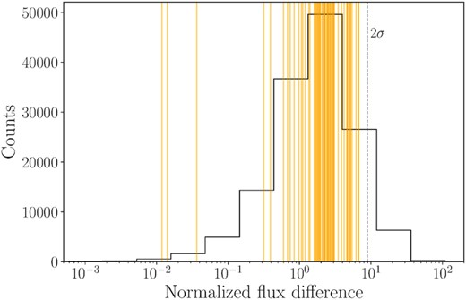
Distribution of source flux difference between images for all persistent sources and normalized by the uncertainties on each flux measurement summed in quadrature. The vertical yellow lines represent the normalized flux difference for 31 transient candidates that passed inspection, and are consistent with the overall source distribution. For reference, a vertical dashed line denoting the 2σ value of the distribution of persistent sources is included.
Our relatively high-sensitivity data of a large field taken at 144 MHz at these three particular epochs presents an opportunity to probe a hitherto unexplored area of transient surface density phase space (Fig. 5). To obtain transient surface density limits, we consider the amount of unique sky sampled (corresponding to the inner 1.4° radius of the LOFAR beams). We calculate the mean rms within this radius for each image. We exclude 2 sub-fields (with right ascensions corresponding to 25.04° and 35.45°, see Table B1) that contained outliers in the image rms comparison. Conservatively taking the maximum mean rms value and multiplying by our detection threshold, we obtain a 7σ survey sensitivity of 20 mJy for 277 deg2 of sky coverage. We follow Rowlinson et al. (2016) to calculate an upper limit on the transient surface density at the 95 per cent confidence level and find 0.01 deg−2 for time-scales corresponding to about one, two, and three months. As can be seen in Fig. 5, this analysis is the most sensitive transient search at low radio frequencies on those time-scales: there are only three other surveys at comparable frequency and time-scales and our data are at least three times more sensitive.
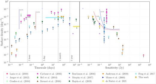
Overview of transient surface densities between about 60 and 340 MHz at time-scales greater than 1 min. The left-hand panel shows the transient surface density as a function of survey time-scale probed, while the right-hand panel shows the surface density as a function of sensitivity probed. The down-facing arrows represent upper limits, whereas data points with no down-facing arrows represent actual transient detections. The limits set by this study are represented by gold stars. A hollow star depicts the median sensitivity (8 mJy) across the 277 deg2 of field used for this analysis (see Section 4.2). This is included in order to compare to Hajela et al. (2019), the next most sensitive survey on month time-scales, which only quotes the median sensitivity. The blue and red lines correspond to limits set by the VLITE survey from Polisensky et al. (2016). A running catalogue of slow radio transient surveys can be found in Mooley et al. (2016). Galactic Centre radio transients have been excluded from this figure.
4.3 Targeted search limits
No transient candidates were found in the neutrino candidate’s error region. The results of forced flux measurements at the location of the UVOT optical transient are summarized in Table 1. Significant radio emission is not detected in any of the three images. That the beam was centred on the position of the optical transient enables us achieve 3σ upper limits down to 1.5 mJy beam−1 without any direction-dependent calibration (DDC). Note that this sub-field unfortunately happens to contain the poorest-quality images of all sub-fields.
Forced measurements at the location of the UVOT optical transient. The location corresponds to the centre of an LOFAR beam. The 3σ limits correspond to three times the local rms value as measured by TraP.
| 3σ limit | Peak flux density | |
|---|---|---|
| Epoch | (mJy beam−1) | (mJy beam−1) |
| 1 | 1.5 | 1.0 ± 0.9 |
| 2 | 1.8 | 2 ± 1 |
| 3 | 4.9 | 4 ± 2 |
| 3σ limit | Peak flux density | |
|---|---|---|
| Epoch | (mJy beam−1) | (mJy beam−1) |
| 1 | 1.5 | 1.0 ± 0.9 |
| 2 | 1.8 | 2 ± 1 |
| 3 | 4.9 | 4 ± 2 |
5 PROSPECTS FOR FUTURE LOFAR GW COUNTERPART SEARCHES
The results presented in this paper demonstrate LOFAR’s ability to provide deep limits over large fields, making it a unique and powerful tool to cover vast swaths of poorly localized GW merger events. In the next GW observing run, the location probability fields are projected to be significantly smaller: the four-detector GW network forecasts median 90 per cent credible regions for the localization area of BNS and BH–NS mergers of 33 ± 5 deg2 and 50 ± 8 deg2, respectively (Abbott et al. 2020). A single LOFAR pointing consisting of seven beams in a hexagonal pattern will cover roughly 40 deg2 at optimum sensitivity (1.4° radius around beam centres) with further coverage away from the centre of the beam pattern. The median sensitivity achieved in this analysis using a 1.4° search radius is 8 mJy. These much smaller field sizes will enable us to reduce the data more carefully and increase data quality. In particular, DDC, which is computationally expensive and unfeasible for fields as large as the one analysed in this work, can be performed. We have purposefully calibrated our data in a way that is compatible with further reduction via KillMS (Tasse 2014a, b; Smirnov & Tasse 2015) and DDFacet (Tasse et al. 2018) or Factor4 for DDC. In particular, KillMS and DDFacet5 are used by the LoTSS surveys team who regularly achieve 70 |$\mu$|Jy beam−1 median rms noise levels for their 8-h integration images (Shimwell et al. 2019). DDC would improve sensitivity and resolution, and should significantly reduce TraP transient false positives by minimizing sidelobe artefacts, which will allow us to relax our search filters and throw a smaller fraction of the sky away in order to decrease the number of candidates. Furthermore, a mosaic of the field can be constructed before searching for transients, to obtain deeper and more uniform sensitivity across the search area. Finally, in cases where an EM counterpart has already been identified, all LOFAR sub-bands can be used to place a single LOFAR beam at its location, thus increasing sensitivity to LoTSS levels (i.e. 3σ sensitivity of 210 |$\mu$|Jy with DDC). An analysis of LOFAR data corresponding to GW triggers detected in O3 is in preparation and will showcase some of the aforementioned improvements and scenarios (Gourdji et al., in preparation).
For GW candidate fields that LoTSS has previously surveyed, we can use LoTSS data as our reference image and compare our later-time LOFAR observations to that catalogue of sources directly to search for GW transients and to perform data quality control (as opposed to performing our own reference observation within a week of the merger and then comparing to TGSS). In that case, the sensitivity of the search described in Section 3.1.2 would be limited by the LOFAR data, rather than by the TGSS catalogue’s much higher 200 mJy completeness threshold. In addition, many of the catalogue comparison challenges discussed in Section 3.1.2 would be diminished or gone altogether.
Broderick et al. (2020) explored the feasibility of using LOFAR to detect the afterglow of GW170817, had the event occurred further north on the sky. They showed that the light-curve, extrapolated to 144 MHz, peaks at about 500 |$\mu$|Jy, thus necessitating DDC. They also considered the scenario where an event similar to GW170817 takes place at a distance of 100 Mpc and in a denser (factor 10) interstellar medium and show that, for various afterglow models, the LOFAR sensitivity would have to be at least 1 mJy, which again requires DDC. The brightness distribution of GW merger afterglows is, however, highly uncertain given the very small sample size and considerable model uncertainties.
Finally, LOFAR can be used to rapidly observe GW triggers within 5 min, to search for related prompt emission. This strategy has been successfully tested with triggered LOFAR observations of gamma-ray bursts (Rowlinson et al. 2019, 2020). LOFAR will be one of few radio facilities capable of probing coherent radio emission at such short time-scales post-merger, and particularly at such sensitivities. For instance, the Murchison Widefield Array (MWA) can be on source within approximately 20 s but is less sensitive than LOFAR by at least an order of magnitude (Anderson et al. 2021). It is as yet unclear whether prompt coherent emission is produced and whether it would be able to escape the merger environment. None the less, a detection would immediately identify the precise location of the merger and would undeniably link compact mergers as a progenitor of FRBs. The recent detection of FRBs with LOFAR shows that they can at least be detected at low frequencies (Pastor-Marazuela et al. 2021; Pleunis et al. 2021).
6 CONCLUSIONS
We have demonstrated a strategy to search for slow transients related to GW merger events in wide-field LOFAR data. In particular, we have presented three different transient search methods involving the comparison to an existing catalogue of radio sources, a blind search between multi-epoch LOFAR images and a targeted search at the location of transients detected at other wavelengths. These methods are telescope agnostic and can be applied to other interferometric radio observations of GW events. We have not found any transients and place the most sensitive transient surface density limits at low radio frequencies to date on time-scales of the order of one month.
We have discussed LOFAR’s prospects for the upcoming GW observing run, and show that LOFAR will be able to probe the full projected median localization area for GW merger events with a single 4-h multibeam observation down to a median sensitivity of 8 mJy, before DDC. Thus, LOFAR will provide the deepest wide-field data sets probing the afterglow of GW merger events at low radio frequencies.
ACKNOWLEDGEMENTS
We thank Mark Kuiack and Iris de Ruiter for helpful discussions. We thank the ASTRON Radio Observatory for setting up the observations used in this paper, and for preprocessing the data.
This paper is based on data obtained with the International LOFAR Telescope (ILT) under project code LC8_005. LOFAR (van Haarlem et al. 2013) is the Low Frequency Array designed and constructed by ASTRON. It has observing, data processing, and data storage facilities in several countries, that are owned by various parties (each with their own funding sources), and that are collectively operated by the ILT foundation under a joint scientific policy. The ILT resources have benefited from the following recent major funding sources: CNRS-INSU, Observatoire de Paris and Université d’Orléans, France; BMBF, MIWF-NRW, MPG, Germany; Science Foundation Ireland (SFI), Department of Business, Enterprise and Innovation (DBEI), Ireland; NWO, The Netherlands; The Science and Technology Facilities Council, UK; Ministry of Science and Higher Education, Poland.
DATA AVAILABILITY
The LOFAR visibility data are publicly available at the LOFAR Long Term Archive (https://lta.lofar.eu/) under project code LC8_005. The derived images used for this article’s analysis will be shared on reasonable request to the corresponding author. A basic reproduction package (10.5281/zenodo.5599729) outlines the data reduction software and settings used in this analysis. It also provides the scripts and data required to reproduce the figures and tables of this paper.
Footnotes
REFERENCES
APPENDIX A: TRANSIENT CANDIDATE EXAMPLE CLASSIFICATIONS
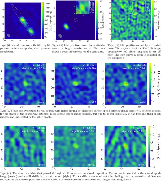
Examples for each of the five new-source candidate types listed and described in Section 3.2. The labels on the x and y axes are in pixel units. All plots are centred on the new-source candidate. The red circle denotes the source position error radius and the yellow ellipse corresponds to the 2D Gaussian source fit as determined by TraP. The restoring beam of each image is shown in the bottom left corner and the pixel size is 5 arcsec.
APPENDIX B: OBSERVATION AND SOURCE COUNT TABLES
Table of observations. The observation start times are shown and the mean image RMS is included.
| RA (deg) | DEC (deg) | Epoch 1 | 〈RMS1〉 | Epoch 2 | 〈RMS2〉 | Epoch 3 | 〈RMS3〉 |
|---|---|---|---|---|---|---|---|
| (UTC) | mJy beam−1 | (UTC) | mJy beam−1 | (UTC) | mJy beam−1 | ||
| 25.035625 | 34.56766667 | a2017-08-31 23:00:05 | 6.2 | 2017-09-24 21:00:05 | 5.4 | 2017-11-20 18:11:05 | 5.1 |
| 27.1051976779 | 37.9065470782 | a2017-08-31 23:00:05 | 2.6 | 2017-09-24 21:00:05 | 3.4 | 2017-11-20 18:11:05 | 2.7 |
| 28.1993407705 | 40.5175129993 | a2017-08-31 23:26:05 | 2.5 | 2017-09-24 21:26:05 | 3.0 | 2017-11-20 18:37:05 | 2.3 |
| 28.2 | 44.8 | 2017-08-30 23:00:05 | 2.8 | 2017-09-23 21:00:05 | 2.0 | 2017-11-18 18:11:05 | 2.7 |
| 29.3066435278 | 35.7780681577 | a2017-08-31 23:00:05 | 3.0 | 2017-09-24 21:00:05 | 2.8 | 2017-11-20 18:11:05 | 2.5 |
| 30.4780083982 | 38.3890340788 | a2017-08-31 23:00:05 | 2.3 | 2017-09-24 21:00:05 | 2.7 | 2017-11-20 18:11:05 | 2.2 |
| 31.320689341 | 78.2892389693 | 2017-09-03 01:26:05 | 2.1 | 2017-09-26 21:37:05 | 1.8 | 2017-11-24 18:37:05 | 3.5 |
| 31.3221270833 | 48.3484145366 | 2017-08-30 23:00:05 | 1.5 | 2017-09-23 21:00:05 | 1.7 | 2017-11-18 18:11:05 | 2.2 |
| 31.5020712805 | 50.8896844781 | 2017-08-30 23:26:05 | 1.6 | 2017-09-23 21:26:05 | 1.6 | 2017-11-18 18:37:05 | 2.0 |
| 31.5080893777 | 33.6495892372 | a2017-08-31 23:00:05 | 3.0 | 2017-09-24 21:00:05 | 3.6 | 2017-11-20 18:11:05 | 3.1 |
| 31.825 | 41.0 | a2017-08-31 23:26:05 | 2.4 | 2017-09-24 21:26:05 | 3.5 | 2017-11-20 18:37:05 | 2.2 |
| 31.990305671 | 81.0651263206 | 2017-09-03 01:26:05 | 2.3 | 2017-09-26 21:37:05 | 1.7 | 2017-11-24 18:37:05 | 3.0 |
| 32.4729327845 | 53.6023540758 | 2017-08-30 23:26:05 | 1.5 | 2017-09-23 21:26:05 | 1.9 | b2017-11-18 18:37:05 | 2.3 |
| 32.5183026084 | 56.2475307662 | 2017-09-04 00:00:05 | 2.6 | 2017-09-27 22:00:05 | 2.6 | 2017-11-25 18:11:05 | 2.8 |
| 32.6794542481 | 36.2605551584 | a2017-08-31 23:00:05 | 2.9 | 2017-09-24 21:00:05 | 3.5 | 2017-11-20 18:11:05 | 2.9 |
| 33.0841782361 | 43.6109659212 | a2017-08-31 23:26:05 | 2.9 | 2017-09-24 21:26:05 | 3.8 | 2017-11-20 18:37:05 | 2.6 |
| 33.4089275424 | 58.9838505214 | 2017-09-04 00:00:05 | 2.7 | 2017-09-27 22:00:05 | 2.7 | 2017-11-25 18:11:05 | 2.9 |
| 33.4320963565 | 61.7201702765 | 2017-09-04 00:26:05 | 2.7 | 2017-09-27 22:26:05 | 2.9 | 2017-11-25 18:37:05 | 3.4 |
| 34.0391514504 | 46.2998659386 | 2017-08-30 23:00:05 | 1.4 | 2017-09-23 21:00:05 | 1.6 | b2017-11-18 18:11:05 | 2.3 |
| 34.1914809934 | 38.8715210795 | a2017-08-31 23:26:05 | 3.0 | 2017-09-24 21:26:05 | 4.3 | 2017-11-20 18:37:05 | 3.1 |
| 34.4830207023 | 64.4564900316 | 2017-09-04 00:26:05 | 2.3 | 2017-09-27 22:26:05 | 2.8 | 2017-11-25 18:37:05 | 3.2 |
| 34.6356226701 | 67.260302694 | 2017-09-03 01:00:05 | 1.8 | 2017-09-26 21:11:05 | 1.7 | 2017-11-24 18:11:05 | 2.4 |
| 35.2485014015 | 48.9497989079 | 2017-08-30 23:00:05 | 1.5 | 2017-09-23 21:00:05 | 1.7 | b2017-11-18 18:11:05 | 2.1 |
| 35.4506592295 | 41.4824870007 | a2017-08-31 23:26:05 | 3.9 | 2017-09-24 21:26:05 | 5.7 | 2017-11-20 18:37:05 | 3.4 |
| 35.7800639102 | 51.725205134 | 2017-08-30 23:26:05 | 1.5 | 2017-09-23 21:26:05 | 1.7 | 2017-11-18 18:37:05 | 2.1 |
| 36.247673704 | 69.9729722917 | 2017-09-03 01:00:05 | 1.6 | 2017-09-26 21:11:05 | 1.5 | 2017-11-24 18:11:05 | 2.3 |
| 36.7509254142 | 54.4378747316 | 2017-08-30 23:26:05 | 1.9 | 2017-09-23 21:26:05 | 2.0 | 2017-11-18 18:37:05 | 2.2 |
| 36.7561758175 | 44.2513173406 | 2017-08-30 23:00:05 | 1.8 | 2017-09-23 21:00:05 | 2.0 | 2017-11-18 18:11:05 | 2.7 |
| 37.3378963963 | 57.1978446442 | 2017-09-04 00:00:05 | 2.9 | 2017-09-27 22:00:05 | 3.1 | 2017-11-25 18:11:05 | 3.4 |
| 37.9655257686 | 46.9012503099 | 2017-08-30 23:00:05 | 1.6 | 2017-09-23 21:00:05 | 1.7 | 2017-11-18 18:11:05 | 2.2 |
| 38.2285213303 | 59.9341643994 | 2017-09-04 00:00:05 | 3.0 | b2017-09-27 22:00:05 | 3.4 | 2017-11-25 18:11:05 | 3.4 |
| 39.0871950358 | 49.8480561921 | 2017-08-30 23:26:05 | 1.7 | 2017-09-23 21:26:05 | 2.0 | 2017-11-18 18:37:05 | 2.4 |
| 39.1191462643 | 62.6704841545 | 2017-09-04 00:26:05 | 2.6 | 2017-09-27 22:26:05 | 2.7 | 2017-11-25 18:37:05 | 3.1 |
| 40.0580565398 | 52.5607257898 | 2017-08-30 23:26:05 | 1.6 | 2017-09-23 21:26:05 | 1.7 | 2017-11-18 18:37:05 | 2.2 |
| 40.1700706101 | 65.4068039096 | 2017-09-04 00:26:05 | 2.1 | 2017-09-27 22:26:05 | 2.6 | 2017-11-25 18:37:05 | 2.9 |
| 41.2668652502 | 55.4118387671 | 2017-09-04 00:00:05 | 2.3 | 2017-09-27 22:00:05 | 2.3 | 2017-11-25 18:11:05 | 2.7 |
| 41.738945248 | 68.0958233498 | 2017-09-03 01:00:05 | 1.7 | 2017-09-26 21:11:05 | 1.7 | 2017-11-24 18:11:05 | 2.4 |
| 42.1574901842 | 58.1481585222 | 2017-09-04 00:00:05 | 2.7 | 2017-09-27 22:00:05 | 3.5 | 2017-11-25 18:11:05 | 2.8 |
| 43.3509962819 | 70.8084929475 | 2017-09-03 01:00:05 | 1.9 | 2017-09-26 21:11:05 | 1.8 | 2017-11-24 18:11:05 | 2.8 |
| 43.7552718262 | 60.8844782774 | 2017-09-04 00:26:05 | 2.3 | 2017-09-27 22:26:05 | 2.5 | 2017-11-25 18:37:05 | 2.8 |
| 44.26788367 | 76.7963348687 | 2017-09-03 01:26:05 | 1.9 | 2017-09-26 21:37:05 | 1.6 | 2017-11-24 18:37:05 | 3.1 |
| 44.8061961721 | 63.6207980325 | 2017-09-04 00:26:05 | 2.0 | 2017-09-27 22:26:05 | 2.3 | 2017-11-25 18:37:05 | 2.5 |
| 44.9375 | 79.57222222 | 2017-09-03 01:26:05 | 2.2 | 2017-09-26 21:37:05 | 1.8 | 2017-11-24 18:37:05 | 3.8 |
| 47.2302167921 | 66.218674408 | 2017-09-03 01:00:05 | 2.1 | 2017-09-26 21:11:05 | 1.6 | 2017-11-24 18:11:05 | 2.5 |
| 48.8422678259 | 68.9313440057 | 2017-09-03 01:00:05 | 1.9 | 2017-09-26 21:11:05 | 1.6 | 2017-11-24 18:11:05 | 2.8 |
| 57.884694329 | 78.0793181194 | 2017-09-03 01:26:05 | 2.1 | 2017-09-26 21:37:05 | 1.8 | 2017-11-24 18:37:05 | 3.6 |
| 58.554310659 | 80.8552054707 | 2017-09-03 01:26:05 | 1.6 | 2017-09-26 21:37:05 | 1.3 | 2017-11-24 18:37:05 | 2.2 |
Data calibrated using 3C 48 instead of 3C 196.
Observations where one of the nine 25-min scans is missing.
Differential source counts corresponding to Fig. 3. From left to right: bin range of flux densities, bin centre flux density, number of sources in bin, correction factor to account for varying sensitivity across the field, and the final Euclidean normalized source density. The uncertainties were calculated following Poisson statistics.
| dFν (Jy) | Fν (Jy) | Raw counts | Completeness weight | Normalized counts (Jy1.5 sr−1) |
|---|---|---|---|---|
| 0.0051–0.0056 | 0.0054 | 84 ± 9 | 141.00 | 29 ± 3 |
| 0.0056–0.0062 | 0.0059 | 117 ± 10 | 80.57 | 27 ± 2 |
| 0.0062–0.0068 | 0.0065 | 241 ± 15 | 37.60 | 30 ± 1 |
| 0.0068–0.0075 | 0.0072 | 380 ± 19 | 23.50 | 34 ± 1 |
| 0.0075–0.0083 | 0.0079 | 582 ± 24 | 16.59 | 42 ± 1 |
| 0.0083–0.0091 | 0.0087 | 850 ± 29 | 10.25 | 44 ± 1 |
| 0.0091–0.010 | 0.0095 | 1177 ± 34 | 6.96 | 48 ± 1 |
| 0.010–0.013 | 0.012 | 5831 ± 76 | 4.15 | 64.5 ± 0.8 |
| 0.013–0.018 | 0.016 | 9784 ± 98 | 2.29 | 92.1 ± 0.9 |
| 0.018–0.024 | 0.021 | 12850 ± 113 | 1.63 | 132 ± 1 |
| 0.024–0.032 | 0.028 | 14745 ± 121 | 1.22 | 175 ± 1 |
| 0.032–0.042 | 0.039 | 16235 ± 127 | 1.05 | 256 ± 2 |
| 0.042–0.056 | 0.049 | 15433 ± 124 | 1.01 | 359 ± 2 |
| 0.056–0.075 | 0.066 | 14223 ± 119 | 1.00 | 505 ± 4 |
| 0.075–0.10 | 0.087 | 11295 ± 106 | 1.00 | 618 ± 5 |
| 0.10–0.13 | 0.12 | 9692 ± 98 | 1.00 | 817 ± 8 |
| 0.13–0.18 | 0.16 | 8629 ± 92 | 1.00 | 1120 ± 12 |
| 0.18–0.24 | 0.21 | 6627 ± 81 | 1.00 | 1325 ± 16 |
| 0.24–0.32 | 0.28 | 5938 ± 77 | 1.00 | 1828 ± 23 |
| 0.32–0.42 | 0.37 | 4352 ± 65 | 1.00 | 2064 ± 31 |
| 0.42–0.56 | 0.49 | 3339 ± 57 | 1.00 | 2438 ± 42 |
| 0.56–0.75 | 0.66 | 2391 ± 48 | 1.00 | 2689 ± 54 |
| 0.75–1.0 | 0.87 | 1914 ± 43 | 1.00 | 3315 ± 75 |
| 1.0–1.3 | 1.2 | 1521 ± 39 | 1.00 | 4056 ± 104 |
| 1.3–1.8 | 1.6 | 773 ± 27 | 1.00 | 3175 ± 114 |
| 1.8–2.4 | 2.1 | 619 ± 24 | 1.00 | 3915 ± 157 |
| 2.4–3.2 | 2.8 | 320 ± 17 | 1.00 | 3116 ± 174 |
| 3.2–4.2 | 3.7 | 200 ± 14 | 1.00 | 2999 ± 212 |
| 4.2–5.6 | 4.9 | 189 ± 13 | 1.00 | 4365 ± 317 |
| 5.6–7.5 | 6.6 | 55 ± 7 | 1.00 | 1956 ± 263 |
| 7.5–10.0 | 8.8 | 61 ± 7 | 1.00 | 3341 ± 427 |
| 10.0–16.2 | 13.1 | 37 ± 6 | 1.00 | 2243 ± 368 |
| 16.2–26.2 | 21.2 | 12 ± 3 | 1.00 | 1499 ± 432 |
| 26.2–42.5 | 34.3 | 18 ± 4 | 1.00 | 4633 ± 1092 |
| 42.5–68.7 | 55.6 | 2 ± 1 | 1.00 | 1060 ± 750 |
