


ABSTRACT
The DES-CMASS sample (DMASS) is designed to optimally combine the weak lensing measurements from the Dark Energy Survey (DES) and redshift-space distortions (RSD) probed by the CMASS galaxy sample from the Baryonic Oscillation Spectroscopic Survey. In this paper, we demonstrate the feasibility of adopting DMASS as the equivalent of CMASS for a joint analysis of DES and BOSS in the framework of modified gravity. We utilize the angular clustering of the DMASS galaxies, cosmic shear of the DES metacalibration sources, and cross-correlation of the two as data vectors. By jointly fitting the combination of the data with the RSD measurements from the CMASS sample and Planck data, we obtain the constraints on modified gravity parameters |$\mu _0=-0.37^{+0.47}_{-0.45}$| and |$\Sigma _0=0.078^{+0.078}_{-0.082}$|. Our constraints of modified gravity with DMASS are tighter than those with the DES Year 1 redMaGiC sample with the same external data sets by 29 per cent for μ0 and 21 per cent for Σ0, and comparable to the published results of the DES Year 1 modified gravity analysis despite this work using fewer external data sets. This improvement is mainly because the galaxy bias parameter is shared and more tightly constrained by both CMASS and DMASS, effectively breaking the degeneracy between the galaxy bias and other cosmological parameters. Such an approach to optimally combine photometric and spectroscopic surveys using a photometric sample equivalent to a spectroscopic sample can be applied to combining future surveys having a limited overlap such as DESI and LSST.
1 INTRODUCTION
Over the past three decades after the discovery of the accelerating Universe (Riess et al. 1998; Perlmutter et al. 1999), the Lambda cold dark matter (ΛCDM) model has been widely accepted as the simplest and the most successful concordance model in modern cosmology. This model is based upon a spatially-flat, expanding Universe governed by Einstein’s General Relativity (GR) and whose components are dominated by roughly 25 per cent of cold dark matter (CDM) and 70 per cent of dark energy, which is commonly associated with a cosmological constant. The cosmological constant, denoted as Λ, can be cast in the model as a perfect fluid with the equation-of-state parameter of minus one in order to trigger the late-time cosmic acceleration. The ΛCDM model has been thoroughly validated through a broad range of stringent tests using cosmological data sets such as the cosmic microwave background (CMB), Type Ia supernovae, baryon acoustic oscillation (BAO), the large-scale clustering of galaxies, and weak gravitational lensing. Despite the overall success of the ΛCDM model supported by many observations, however, several fundamental puzzles remain. One notable concern is that the cosmological constant has no explicit physical theory for its origin. In the context of quantum field theory, one may connect the cosmological constant with the vacuum energy associated with zero-level quantum fluctuations. However, this approach can be easily countered by ∼120 orders of magnitude difference in the value of the vacuum energy predicted by quantum field theory and inferred from the LCDM model (Weinberg 1989). Such discrepancy leads to the desire for alternative models beyond the ΛCDM cosmology.
Modified gravity (MG) has been suggested as one of the strong candidates to explain the cosmic acceleration without introducing a cosmological constant. In such a theory, modified GR at cosmological scales naturally produces an acceleration identical to the one assumed in the ΛCDM model, without raising the same issues as a cosmological constant. In a phenomenological approach, the modification to GR is often parametrized as two MG parameters added to the gravitational potentials in the Friedmann equations. These MG parameters modify the growth equations derived from the Friedmann equations, and thereby any departure from GR appears as a change in the growth of structure and the deflection of light while keeping the same expansion history of the Universe as ΛCDM (see Ishak 2019, for an overview of the theory and phenomenology of MG models). Hence, it is worth noting that probes sensitive to the growth of structure play a crucial role in testing deviations from GR.
Redshift space distortions (RSD) and weak gravitational lensing have been used together as a popular combination of growth data to test GR (Zhang et al. 2007; Reyes et al. 2010; Simpson et al. 2013; Blake et al. 2016; de la Torre et al. 2017; Abbott et al. 2019; Ferté et al. 2019; Singh et al. 2019; Planck Collaboration VI 2020a). A general approach to combine these two probes is adding an independent measurement of f(z)σ8(z) from redshift-space distortions by a spectroscopic survey to a weak lensing measurement by a photometric survey. However, several papers (Bernstein & Cai 2011; Cai & Bernstein 2012; Gaztañaga et al. 2012) have shown that a combined analysis of overlapping spectroscopic and weak lensing surveys can yield much stronger dark energy and growth constraints than a combination of independent RSD and weak lensing measurements. The motivation for combining those two overlapping probes comes from the fact that RSD provides the constraints of the growth parameters only in combination with other parameters, i.e. the measurements of f(z)σ8(z) and β = f(z)/b where f(z) is the redshift-dependent growth rate, σ8(z) is the amplitude of the matter clustering at redshift z, and b is galaxy bias. Galaxy bias has been a major source of uncertainty in cosmological analyses of large-scale structure. In the MG framework, its impact is even more significant because one of the MG parameters modifying the Newtonian potential enters into σ8(z) and f(z) through the growth factor term and is strongly degenerate with galaxy bias. Without any prior knowledge of galaxy bias, one cannot constrain f(z) or σ8(z) independently, resulting in the degradation of the measurement of MG parameters.1 Meanwhile, weak gravitational lensing directly measures the value of σ8 today. The cross-correlation of RSD and weak lensing enables us to tighten the constraint of galaxy bias by breaking the f–b degeneracy and allows a more precise inference of the underlying distribution of matter.
Several studies have taken the aforementioned approach to test GR by combining the RSD measurements from the Baryonic Oscillation Spectroscopic Survey (BOSS; Eisenstein et al. 2011) and weak lensing measurements from recent deep imaging surveys such as the Canada–France–Hawaii Telescope Lensing Survey (CFHTLenS; Heymans et al. 2012), Dark Energy Survey (DES; Abbott et al. 2016), Kilo-Degree Survey (KiDS; de Jong et al. 2013) and the Hyper Suprime-Cam Survey (HSC; Aihara et al. 2018). The BOSS target galaxy samples, LOWZ and CMASS (Reid et al. 2016), are the largest galaxy spectroscopic samples yielding the best BAO and RSD measurements in the redshift range of 0.15 < z < 0.75. The large sample size and the availability of spectroscopic redshifts have turned the galaxies in the samples into a popular candidate for gravitational lenses in the overlapping regions with the imaging surveys. By adopting BOSS galaxies as lenses, one can access better deep images while maintaining the strong constraining power of the galaxy clustering measurements from BOSS.
Alam et al. (2017a) tested gravity by combining galaxy–galaxy lensing from CFHTLenS (Miyatake et al. 2015) with redshift space galaxy clustering from the BOSS CMASS sample (Alam et al. 2015). The galaxy–galaxy lensing signal was obtained around the CMASS galaxies living in the small overlapping area of |$105 {\rm \, deg^2}$| between the BOSS and CFHTLenS footprints. Jullo et al. (2019) performed a similar analysis with the addition of a shape catalogue from CFHT-Stripe 82 (Moraes et al. 2014) to extend the available area for weak lensing to |$250 {\rm \, deg^2}$|. Unlike the previous cases, the KiDS survey was intentionally designed to mostly overlap with the BOSS and 2dFLenS surveys to maximize the number of reliable spectroscopic lenses in their full footprint (de Jong et al. 2013). Joudaki et al. (2017) and Amon et al. (2018) fully utilized the KiDS-450 footprint (|$450 \deg ^2$|) to test gravity in a phenomenological approach using the BOSS galaxies as lenses on the KiDS imaging data. Later, Tröster et al. (2020) constrained the f(R) gravity model with the BOSS galaxies over the KiDS-1000 footprint covering the increased area of |$\sim 1000 {\rm \, deg^2}$|. As shown in these previous studies, however, the MG analyses performed with the spectroscopic samples have to face a limitation due to a fairly small overlapping region with spectroscopic surveys (mostly within a few hundreds of |${\rm \, deg^2}$|), unless imaging surveys are planned in consideration of utilizing the existing spectroscopic information such as KiDS.
The DES-CMASS galaxy sample from the Dark Energy Survey (hereafter DMASS) has been developed to optimally combine the measurements of weak lensing from DES and RSD from BOSS by extending the available area for such analyses beyond the overlap between BOSS and DES (Lee et al. 2019). The selection algorithm for DMASS is trained in the overlapping region (|$123 \deg ^2$|) with galaxy colours and magnitudes, and then identifies CMASS-like galaxies in the rest of the DES footprint where the spectroscopic information is not available. The resulting DMASS sample replicates the statistical properties of the CMASS galaxy sample and populates the lower region of the DES Year 1 (Y1) wide-area survey footprint (|$1244 \deg ^2$|), excluding the overlap. Using the DMASS galaxies as lenses, one can obtain the measurements of galaxy clustering and galaxy–galaxy lensing equivalent to those that would have been measured if CMASS populated the full footprint of DES. These two clustering measurements, along with cosmic shear (the correlation of galaxy shapes) from the DES source galaxies, not only extract the full statistical power of DES, but they can also be efficiently combined with the measurement of redshift-space distortion from CMASS without introducing additional systematics parameters such as galaxy bias.
In this paper, we test the feasibility of this optimal combination method using the DMASS galaxy sample as lenses in the framework of phenomenological modified gravity. To isolate the results from any additional complexity arising from different probes, we adopt a minimal set of data as follows: the combination of angular galaxy clustering, cosmic shear, and the cross-correlations of the two (galaxy–galaxy lensing) measured with the DMASS lenses and DES Y1 sources (hereafter DMASS 3x2pt), the RSD and BAO measurements from the BOSS CMASS sample (Chuang et al. 2017), and Planck 2018 data (Planck Collaboration VI 2020a). The measurement of angular galaxy clustering used in this work is described in the original sample paper (Lee et al. 2019). The measurement of galaxy–galaxy lensing and its calibration procedures are detailed in Lee et al. (2021). DES Y1 cosmic shear is adopted from Troxel et al. (2018). Note that we define ‘DMASS 3x2pt + CMASS RSD/BAO’ as a baseline as DMASS is designed to harness its maximum power in combination with CMASS. In Fig. 1, we summarize the data sets used in the analysis. We follow the methodology used in the DES Y1 analysis for modified gravity (hereafter DESY1MG; Abbott et al. 2019) and compare their MG constraints with ours to estimate the efficiency of this method.
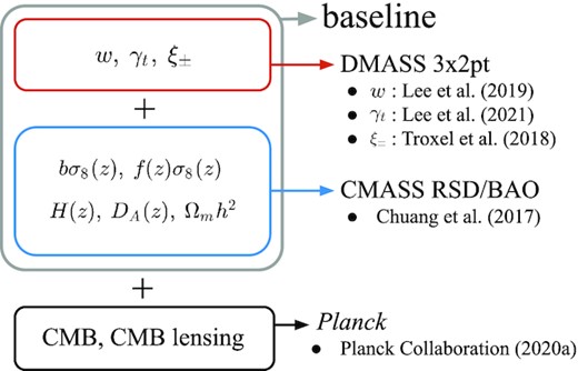
Summary of the different data sets in this analysis. The data in this paper consist of the DMASS 3x2pt measurements, the RSD and BAO measurements from the BOSS CMASS sample, and the CMB measurement from Planck. The DMASS 3x2pt measurement in the red box includes angular clustering (w), cosmic shear (ξ±), the cross-correlation of the two (galaxy–galaxy lensing, γt) measured with the DMASS lenses and the DES Y1 metacalibration sources. The measurement from CMASS provides five constraints on RSD and BAO in the blue box. See Section 3.2 for a detailed description for these parameters. The combination of the red and blue boxes is defined as ‘baseline’. The galaxy bias parameter (b) is shared in this combination. The black box represents the CMB and CMB lensing measurements from Planck (see Section 3.3).
This paper is organized as follows. In the following section, we introduce the phenomenological parametrization of MG adopted in this paper. The data sets and theoretical predictions used to describe the data are detailed in Section 3. In Section 4, we describe our analysis methodology. In Section 5, we present a series of validation tests for potential systematics that might bias the results. In Section 6, we briefly describe how we blind the data to avoid confirmation bias. In Section 7, we present our results and compare them with the results of DESY1MG. Our conclusions are presented in Section 8.
2 PARAMETRIZATION OF MODIFIED GRAVITY
We parametrize departures from GR in a phenomenological way. This approach has an advantage in the sense that it does not require exact knowledge of the specific alternative theory but is still able to capture a generic deviation of the perturbation evolution from ΛCDM, by injecting two parameters into the perturbed Einstein’s equations (see Ishak 2019, for a general overview of the phenomenological approach and its applications).
3 DATA AND MEASUREMENTS
In this section, we explain the data sets and measurements we use for the analysis. The primary data used in this work are the DMASS galaxy catalogue (Lee et al. 2019) and metacalibration shape catalog (Zuntz et al. 2018) from DES. Both catalogues are based on the images taken between 2013 August 31 and 2014 February 9 during the first year observations of DES (Abbott et al. 2005; Flaugher et al. 2015; Abbott et al. 2018). In Section 3.1, we briefly describe the two catalogs and the 3 × 2 pt measurements (galaxy clustering, tangential shear, and cosmic shear) obtained with these catalogs. We also utilize the RSD and BAO measurements extracted from the galaxy clustering of the BOSS CMASS galaxies (Chuang et al. 2017). Their measurements and corresponding covariance matrices are presented in Section 3.2. In Section 3.3, we briefly describe the Planck CMB data we include to constrain the early universe.
3.1 Dark Energy Survey
3.1.1 DMASS and metacalibration catalogues
We utilize the DMASS galaxy sample (Lee et al. 2019) as gravitational lenses. The DMASS sample is a photometric sample designed to replicate the statistical properties of the BOSS CMASS galaxy sample (Reid et al. 2016). The sample consists of 117 293 effective galaxies selected from the DES Y1 GOLD catalog (Drlica-Wagner et al. 2018), and covers the lower region of the DES Y1 wide-area survey footprint, excluding the overlapping area with BOSS near the celestial equator. The full coverage of DMASS is |$1,244 {\rm \, deg^2}$| after masking.
The feasibility of using the DMASS sample as an equivalent of the CMASS sample has been studied in Lee et al. (2019) and Lee et al. (2021). In Lee et al. (2019), the redshift distribution of DMASS was computed by cross-correlating the sample with the DES Y1 redMaGiC galaxy sample (Rozo et al. 2016; Elvin-Poole et al. 2018). Fig. 2 shows the redshift distributions of CMASS (red shaded region) and DMASS (maroon error bars). The two distributions show good agreement.2 Therefore, we use the redshift distribution of CMASS as the true redshift distribution for a theoretical prediction for DMASS. In addition, Lee et al. (2019) showed the consistency between DMASS and CMASS by comparing various statistical properties such as the number density, auto-angular clustering, and cross-angular clustering with the external surveys. The resulting values of the difference in the mean galaxy bias and mean redshift are |$\Delta b = 0.044^{+0.044}_{-0.043}$| and |$\Delta z = (3.51 ^{+4.93}_{-5.91}) \times 10^{-3}$|, which indicate that the galaxy bias and mean redshift of two samples are consistent within 1σ. For more description of the galaxy sample and sample selection algorithm, we refer readers to Lee et al. (2019).
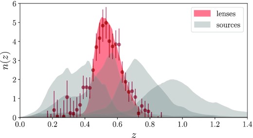
The spectroscopic redshift distribution of BOSS CMASS (red shaded) and the photometric redshift distributions of metacalibration (grey shaded). The maroon colour points with error bars show the redshift distribution of DMASS computed by cross-correlating the sample with the DES Y1 redMaGiC sample. As the redshift distributions of CMASS and DMASS show good consistency, we use the redshift distribuion of CMASS as the true redshift distribution for a theoretical prediction for DMASS. The source sample, metacalibration is divided into four tomographic bins (0.2 < zs < 0.43, 0.43 < zs < 0.63, 0.63 < zs < 0.90 and 0.90 < zs < 1.30) using the BPZ photometric redshift code.
Source galaxies are selected from the DES metacalibration catalogue (Huff & Mandelbaum 2017; Sheldon & Huff 2017; Zuntz et al. 2018). Photo-z of individual galaxies are evaluated by the Bayesian Photometric Redshift (BPZ) algorithm (Coe et al. 2006; Hoyle et al. 2018). As in Zuntz et al. (2018), Prat et al. (2018), and Troxel et al. (2018), sources are split into four redshift bins selected using BPZ: 0.2 < z < 0.43, 0.43 < z < 0.63, 0.63 < z < 0.90, and 0.90 < z < 1.30. The redshift distributions of the four source bins are plotted in Fig. 2 with the redshift distribution of lenses. The shear multiplicative biases, photo-z biases, and their uncertainties related to this catalogue are quantified in Zuntz et al. (2018), Hoyle et al. (2018) and employed as priors in our analysis. See Section 4 for a detailed description.
We do not split the lens sample in multiple redshift bins. Instead of using the five tomographic lens bins as done in DESY1MG, we consider only one lens bin along with the four source bins. This choice of one tomographic lens bin is motivated by the two reasons as follows. First, Chuang et al. (2017) split the LOWZ and CMASS sample into two bins (for a total of four bins) to increase the sensitivity of redshift evolution, but did not find improvement in terms of constraining different dark energy model parameters compared to the case of one bin. Secondly, splitting the DMASS sample into multiple redshift bins requires retraining the DMASS algorithm, and a series of validation tests performed in Lee et al. (2019) should be followed. The combination of the one lens and four source bins results in one galaxy clustering signal, four galaxy–galaxy lensing signals, and twenty shear signals. In the following sections, we will describe the modelling and measurement of these two-point functions.
3.1.2 Angular galaxy clustering
Lee et al. (2019) computed the angular clustering of DMASS to verify the consistency between DMASS and CMASS. By following the procedure described in that paper, we recompute the signal in the same manner, but with the number of angular bins increased from 10 to 20. The measurement of w(θ) is displayed in the first panel of Fig. 3 with the best-fitting MG prediction. As we obtained the same result except for the number of bins, we only briefly summarize the methodology below and refer readers to Lee et al. (2019) for details.
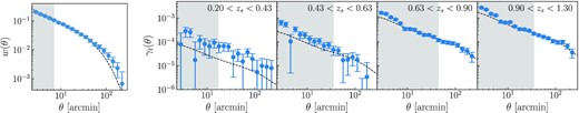
The angular galaxy clustering (left) and tangential shear data (right) from Lee et al. (2019) and Lee et al. (2021). The signals are measured with the DMASS (lenses) and DES Y1 metacalibration (sources) catalogs. The dashed lines are the best-fitting MG predictions from the combination of the baseline case (DMASS 3x2pt + CMASS RSD/BAO) and Planck data. The shaded regions are discarded in the analysis to exclude the small scales where the phenomenological parametrization is not valid. The remaining data points are 16 points for w(θ) and 38 points for γt(θ).
3.1.3 Galaxy–galaxy lensing
3.1.4 Cosmic shear
We utilize the shear measurement from Troxel et al. (2018) obtained with the DES metacalibration galaxies. Troxel et al. (2018) present the auto- and cross-correlation functions |$\xi _{\pm }^{ij}(\theta)$| of the source galaxies divided into four redshift bins over scales 2.5 arcmin < θ < 250 arcmin. Systematics related to the source catalog are parametrized in the same manner as described in Troxel et al. (2018). Fig. 4 shows the measurements of ξ±(θ). The bottom triangle contains ξ+(θ) and the top triangle contains ξ−(θ). The dashed lines are the best-fitting MG predictions from the combination of the DMASS 3 × 2 pt, CMASS RSD/BAO, and Planck data. The labels (i, j) in the upper-right corner of each panel indicate the combination of the ith and jth source tomographic bins used to obtain each signal. The lowest index indicates the lowest tomographic bin. See Troxel et al. (2018) for a detailed description.
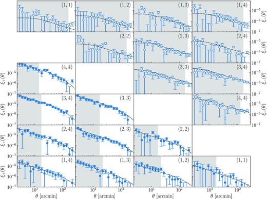
The cosmic shear data from Troxel et al. (2018) measured with the DES Y1 metacalibration catalog. The bottom triangle contains ξ+(θ) and the top triangle contains ξ−(θ). The dashed lines are the best-fitting MG predictions from the combination of the baseline case and Planck data. The labels (i, j) in the upper-right corner of each panel indicate the combination of the ith and jth source tomographic bins used to obtain each signal. The shaded regions are discarded for the cosmological analysis, leaving 119 points for ξ+(θ) and 38 points for ξ−(θ).
3.1.5 Angular scale cuts
The phenomenological approach such as the μ, Σ parametrization is based on the linearly perturbed Einstein equations, so the scales should be limited to the linear regime only. To deal with the nonlinear scales accurately, using either semi-analytical methods or N-body simulation based on a specific MG model is necessary.
Following the Planck 2018 analysis (Planck Collaboration VI 2020a), we restrict ourselves to observables sensitive to the linear scales only. We compute the difference between the nonlinear and linear-theory predictions in the standard LCDM model in our fiducial cosmology as Δχ2 = (dnl − dlin)TC−1(dnl − dlin). The nonlinear predictions are obtained using halofit (Takahashi et al. 2012) implemented in CosmoSIS. Then, we identify the single data point that contributes most to this quantity, and remove that data point, iterating until the quantity reaches Δχ2 < 1. The shaded regions in Figs 3 and 4 indicate the data points removed. Through this process, we obtain 119 data points for ξ+(θ), 18 points for ξ−(θ), 38 points for γt(θ), and 16 points for w(θ).
3.1.6 Covariance
Our measurements of w(θ), γt(θ), and ξ±(θ) are correlated across angular and source redshift bins. The joint covariance for these measurements is computed by cosmoLike (Krause & Eifler 2017) using the halo-based approach (Cooray & Sheth 2002), assuming a ΛCDM cosmology. The covariance is calculated as the sum of Gaussian covariance, non-Gaussian covariance, and the super-sample covariance as described in Krause et al. (2017).
We assume there is no cross-correlation between surveys as the DES and BOSS areas used do not overlap,3 and the CMB data are most sensitive to higher redshift than the galaxy surveys are. The galaxy surveys also form a small fraction of the full-sky CMB measurements.
3.2 RSD and BAO measurements from BOSS CMASS
Redshift space distortions (RSDs) are one of the most promising probes for testing gravity. On large scales, peculiar velocities of galaxies follow infall of matter towards high-density regions (Kaiser 1984), and through that, they are sensitive to the growth rate of structure.
The measurements of RSD that we use in this study are derived from the Baryon Oscillation Spectroscopic Survey (BOSS; Eisenstein et al. 2011; Bolton et al. 2012; Dawson et al. 2013). BOSS targeted two distinct samples known as LOWZ at 0.15 < z < 0.43 and CMASS at 0.43 < z < 0.75 (Reid et al. 2016). The higher redshift sample, CMASS, was designed to select a stellar mass-limited sample of objects of all intrinsic colours, with a colour cut that selects almost exclusively on redshift (Reid et al. 2016). The DMASS sample we use as lenses is designed to mimic this sample. Chuang et al. (2017) present cosmological constraints from galaxy clustering of the LOWZ and CMASS samples. They provide the growth rate and mean galaxy bias combined with the amplitude of mass fluctuation (f(z)σ8(z) and b(z)σ8(z)) at different redshift points.4 In this work, we utilize their results measured at the mean redshift of CMASS (z = 0.59). The galaxy bias parameter b here is shared with the galaxy bias incorporated in the angular galaxy clustering and tangential shear of DMASS.
We also utilize the BAO measurements from the same work to constrain the geometry of the background universe. The BAO measurements chosen are the constraints of the Hubble parameter (H(z)), the comoving angular diameter distance (dA(z)) at the mean redshift of CMASS (z = 0.59), and the matter density fraction (Ωmh2).
We use the full covariance matrix between those RSD and BAO parameters given in the same work.
3.3 CMB and CMB lensing
CMB is one of the most powerful cosmological probes. Through its primary anisotropies such as temperature and polarization power spectra, the CMB tightly constrains the background geometry and the initial conditions. The secondary anisotropies such as the Integrated Sachs–Wolfe–Effect (ISW) and the CMB lensing at late times are more relevant to scalar mode perturbations and the growth of large-scale structure.
The ISW effect is caused by time variations in the gravitational potentials (Sachs & Wolfe 1967). When CMB photons travel from the surface of the last scattering to us, they gain energy while falling down gravitational potential wells, but they lose it again while climbing out of the potential wells. However, dark energy components or modifications to gravity can cause stretching in the potential well, resulting in a net gain in energy for the photons during their journey through the potential wells.
CMB lensing refers to the deflections of CMB photons by the intervening matter while traveling from the surface of last scattering to us. Hence, CMB lensing is sensitive to the distribution and growth rate of large-scale structures and their associated gravitational potential. The deflections of CMB photons smear out the CMB temperature power spectra and also induce non-Gaussianities in the temperature and polarization maps (Bernardeau 1998; Zaldarriaga & Seljak 1998; Okamoto & Hu 2003).
In this work, we utilize the Planck 2018 likelihood described in Planck Collaboration VI (2020a). We use the Planck temperature and polarization auto- and cross-multipole power spectra denoted as |$C^{TT}_{\ell }, C^{TE}_{\ell }, C^{EE}_{\ell }$|, and |$C^{BB}_{\ell }$|. Specifically, we use the full range of |$C^{TT}_{\ell },C^{TE}_{\ell }, C^{EE}_{\ell }$| from 29 < ℓ < 2509 and the low-ℓ polarization data including |$C^{BB}_{\ell }$| from 2 < ℓ < 29. We also make use of the Planck CMB lensing likelihood from temperature only (Planck Collaboration VIII 2020b).
4 ANALYSIS
In this section, we describe our methodology of measuring the cosmological constraints in the framework of modified gravity.
To compute a theoretical prediction, we use CosmoSIS5 (Zuntz et al. 2015) with a version of MGCamb6 (Zhao et al. 2009; Hojjati, Pogosian & Zhao 2011; Zucca & Pogosian et al. 2019; Lewis, Challinor & Lasenby 2000) modified to include the Σ and μ parametrization. We utilize the halofit prescription (Takahashi et al. 2012) to compute the nonlinear power spectrum.
We perform Markov Chain Monte Carlo likelihood analyses using the multinest algorithm (Feroz & Hobson 2008; Feroz, Hobson & Bridges 2009; Feroz & Hobson et al. 2019) implemented in the CosmoSIS package. Our analysis spans the parameter set {Ωm, h0, Ωb, ns, As, (τ, Ων)} where the parentheses around the optical depth parameter and the neutrino density indicate that they are used only in the analysis combinations that use the CMB data. In addition to this set of ΛCDM parameters, we vary {μ0, Σ0} to test gravity. Along with the parameter set, we also vary nuisance parameters describing the photo-z and shear systematics for different tomographic bins, and model parameters for the intrinsic alignment. Since we use the identical source sample as DESY1MG, we adopt the same models for the shear and photo-z systematics (Krause et al. 2017). The complete set of varied parameters and priors is summarized in Table 1. The priors imposed in this analysis are identical to those of DESY1MG except for the lens galaxy bias (b) and lens redshift bias (Δzlens), summarized below.
Lens galaxy bias (b): The linear galaxy bias parameter for lenses. Since we select fairly large scales where the linear assumption is valid, we use a constant galaxy bias over the redshift range. The redshift evolution of CMASS and DMASS is negligible, which is illustrated in Salazar-Albornoz et al. (2017) and Lee et al. (2019). The scale-independence of the DMASS galaxy bias over the scales of interest is shown in Lee et al. (2021). The galaxy bias parameter is shared with the galaxy bias in bσ8 from the BOSS measurements described in Section 3.2.
Lens redshift bias (Δzlens): We model the redshift distribution of lenses as |$n_{\rm true}(z) = \hat{n}(z - \Delta z_{\rm lens})$|, where |$\hat{n}$| is the measured redshift distribution, and Δzlens is a redshift bias parameter. Lee et al. (2019) constrained Δzlens by jointly fitting the residuals of the angular correlation and clustering-z measurements, and obtained Δz = 3.5 × 10⁻⁴ with its uncertainty of σΔz = 0.5 × 10⁻³. We take those values as the mean and width of a Gaussian prior, respectively.
Parameters and priors used to describe the measured galaxy–galaxy lensing signal. ‘Flat’ is a flat prior in the range given while ‘Gauss’ is a Gaussian prior with mean μ and width σ. Priors for the tomographic shear and photo-z bias parameters mi and |$\Delta z_{\rm src}^i$| are identical to DESY1MG.
| Parameter | Notation | Fiducial | Prior |
|---|---|---|---|
| Normalized matter density | Ωm | 0.306 | Flat (0.1, 0.9) |
| Normalized baryon density | Ωb | 4.845 × 10⁻² | Flat (0.03, 0.07) |
| Amplitude of primordial power spectrum | As | 2.196 × 10⁻⁹ | Flat (5 × 10⁻¹⁰, 5 × 10⁻⁹) |
| Power spectrum tilt | ns | 0.968 | Flat (0.87, 1.07) |
| Hubble parameter (H0 = 100h) | h | 0.678 | Flat (0.55, 0.90) |
| Normalized neutrino density | Ων | 6.50 × 10⁻⁴ | Flat (5 × 10⁻⁴, 10−2) |
| Optical depth | τ | 0.081 | Flat (0.01, 0.20) |
| Modified gravity parameter | μ0 | 0.0 | Flat (-3.0, 3.0) |
| Modified gravity parameter | Σ0 | 0.0 | Flat (-3.0, 3.0) |
| Linear galaxy bias (lens) | b | 2.0 | Flat (0.8, 3.0) |
| Intrinsic alignment amplitude | AIA | 0.0 | Flat (−5.0, 5.0) |
| Intrinsic alignment scaling | ηIA | 0.0 | Flat (−5.0, 5.0) |
| Lens redshift bias | Δzlens | 0.0035 | Gauss (0.0035, 0.005) |
| Source photo-z bias (i = 1) | |$\Delta z^1_{\rm src}$| | −0.001 | Gauss (−0.001, 0.016) |
| Source photo-z bias (i = 2) | |$\Delta z^2_{\rm src}$| | −0.009 | Gauss (−0.009, 0.013) |
| Source photo-z bias (i = 3) | |$\Delta z^3_{\rm src}$| | 0.009 | Gauss (0.009, 0.011) |
| Source photo-z bias (i = 4) | |$\Delta z^4_{\rm src}$| | −0.018 | Gauss (−0.018, 0.022) |
| Shear calibration bias (i ∈ {1, 2, 3, 4}) | mi | 0.012 | Gauss (0.012, 0.023) |
5 ROBUSTNESS TESTS
In this section, we perform a series of tests to show the robustness of our results to modeling assumptions and approximations. We thoroughly follow the procedures illustrated in DESY1MG. First, we generate a set of simulated data vectors of w(θ), γt(θ), and ξ±(θ) shifted with the addition of a systematic effect that is not included in our analysis pipeline. Then, each of the simulated data vectors is individually analysed with our fiducial pipeline by using the methodology described in Section 4. Finally, we compare the inferred values of cosmological parameters from the simulated data vectors to the fiducial values. Following DESY1MG, we adopt 1σ as the threshold for a bias. If we observe a bias shifted more than 1σ from the fiducial quantity, the corresponding effect of systematics or modelling assumption needs to be corrected or adequately accounted for in our analysis pipeline.
The modelling assumptions that we consider are summarized below:
Limber approximation and RSD: The Limber approximation (Limber 1953, 1954) enables us to compute the angular two-point statistics efficiently by simplifying the Bessel function integrals. However, this approximation may not be sufficient if the constraining power from surveys can no longer tolerate the errors induced by the approximation. We simulate a data vector using the exact w(θ) calculation and include the contribution from redshift space distortions (Padmanabhan et al. 2007).
Magnification: The observed number density of foreground galaxies can be altered due to the matter between the foreground galaxies and the observer, leading to a systematic bias to the two-point statistics. For the foreground redshift z > 0.45, the effect can bias the inferred dark energy equation of state by more than 5 per cent (Ziour & Hui 2008). Accounting for this effect is critical for the higher redshift samples, such as DMASS. To estimate the impact of the magnification bias, we simulate a data vector by injecting the contribution of magnification to γt(θ) and w(θ). We assume that the change in the observed galaxy overdensity for lenses produced by magnification is proportional to the convergence field of lenses. This can be expressed as |$\delta _g^{\rm obs} = \delta _g^{\rm int} + 2(\alpha - 1) \kappa$|, where |$\delta _g^{\rm int}$| is the galaxy over-density that would have been observed in the absence of magnification, α is the logarithmic slope of the luminosity function of lenses at its faint end, and κ is the convergence of the lenses (Bartelmann & Schneider 2001). We adopt the value of α = 2.62 computed using the CMASS galaxy mocks in Joachimi et al. (2020).
Intrinsic alignments: Our fiducial pipeline accounts for the tidal alignment of massive elliptical galaxies on large scales. However, the contribution from ‘tidal torquing’ induced by spiral or less luminous elliptical galaxies is non-negligible on smaller scales. We simulate a data vector using the Tidal Alignment and Tidal Torquing model (TATT) described in Blazek et al. (2019). We set the TATT amplitudes to A1 = 0, A2 = 2 with no z dependence as done in Abbott et al. (2018) and DESY1MG. This choice of TATT parameters corresponds to testing the impact of a pure tidal torquing model when analyzed with a tidal alignment model.
Since we cut out the majority of the nonlinear scales as described in Section 3.1.5, we do not consider systematics that particularly affects small scales such as baryonic feedback effects. We do not test for the nonlinear galaxy bias either as the linearity of the galaxy bias of DMASS on galaxy clustering and galaxy–galaxy lensing has been verified in Lee et al. (2019, 2021) down to the scales of |$4\, h^{-1}\, {\rm Mpc}$|. These tests have been performed by jointly fitting the two-point statistics with other external probes. DESY1MG tested the aforementioned systematics using their 3 × 2 pt simulated data vector and external data sets. For the case of the 3 × 2 pt simulated data vector only, their posteriors of modified gravity were skewed from true values due to the interplay of weak constraining power with a relatively flat likelihood profile and prior volume effect. As we use only one lens bin compared to DES Y1 five bins, we should expect a worse bias in the posteriors with weaker constraining power. Therefore, we perform the systematics tests by jointly fitting the two-point statistics with the simulated BOSS CMASS likelihood. Since the simulated BOSS CMASS likelihood is not sensitive to any of the systematics correlated with the two-point functions, bias from the fiducial values is solely originating from the two-point functions of DMASS. We also perform the systematics tests including the actual Planck data set as shifts by systematics may appear with higher constraining power.
The results of the robustness tests are shown in Fig. 5, for the two modified gravity parameters (μ0, Σ0) and the parameters that are most sensitive to in this work: Ωm, S8, b. The top panel shows the constraints obtained from the baseline case, and the bottom panel shows the baseline + Planck case. The different rows correspond to the different systematics described above. The topmost error bars in each panel are our fiducial case. For all cases, our posteriors for these cosmological parameters remain well within 1σ of the fiducial constraints.
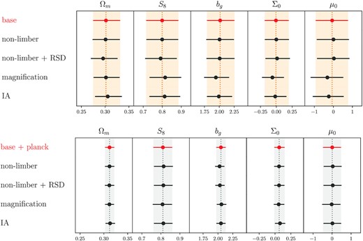
Marginalized 1D posterior constraints on Ωm, S8, b, Σ0, μ0 obtained from DMASS 3 × 2 pt + CMASS RSD/BAO (baseline; top) and DMASS 3x2pt + CMASS RSD/BAO + Planck (bottom). The different rows correspond to the different systematics injected in each of the simulated data vectors. The systematics tested here are detailed in Section 5. These data vectors are analysed by the fiducial pipeline to test the impact of systematics associated with each data vector on the parameter constraints. For all cases, the posteriors for these cosmological parameters remain well within 1σ of the fiducial constraints.
Throughout the robustness tests, we use an importance sampling pipeline (Weaverdyck et al. in preparation) to rapidly compute posterior means for each systematics. For a given sample from a proposal distribution, the importance sampling pipeline draws the expected values of parameters under a target distribution by weighting points with density ratios of the proposal distribution and target distribution, called importance weights. We adopt the effective number of samples as a diagnostic tool to evaluate the accuracy of importance sampling, which is given as |$N^{\rm IS}_{\rm eff} = 1 / \sum ^{N}_{i=1} w_i^2$|, where N is the total sample size and wi represents normalized importance weights. If the proposal distribution is equal to the target distribution, the quantity becomes |$N^{\rm IS}_{\rm eff} = N$|. We determine |$N^{\rm IS}_{\rm eff}/N \gt 0.7$| as the threshold of reliability and evaluate the quantity for each systematics chain obtained by the importance sampler. We find that all of the systematics chains pass the threshold except for the case of intrinsic alignments. Therefore, we use multinest for the intrinsic alignments and utilize the importance sampler for the rest of the systematics.
6 BLINDING
We blinded our results in the parameter-level to avoid confirmation bias. The measurements of γt from Lee et al. (2021) were blinded in the real data analysis. No comparison to theoretical predictions at the two-point level was made in the blinding stage. The cosmological parameter constraints were scaled and shifted by a random number when plotting. After ensuring that there were no major systematics that can bias the cosmological constraints through a series of robustness tests listed in Section 5, we unblinded both the data vector of γt and cosmological constraints. As described in the next section, after unblinding we performed an additional test to estimate the impact of the high signal of γt measured with the first source bin that was detected after unblinding. No change was made in either the analysis method or pipeline after unblinding.
7 RESULTS
7.1 Constraints on modified gravity
In this section, we show the resulting MG constraints obtained from the various combinations of the data sets listed in Section 3. For all cases reported, we include the CMASS likelihood to DES 3 × 2 pt as default and do not report the result from DMASS alone because (1) DMASS is designed to harness its maximum power when its measurements are combined with the measurements of CMASS, and (2) DMASS only, without the help of external data sets, suffers from a projection bias in the posteriors of modified gravity as stated in Section 5.
Fig. 6 shows the resulting constraints in the μ0–Σ0 plane (left) and Ωm–S8 plane (right). Table 2 presents a more detailed summary on our findings, including the constraint of galaxy bias. In Fig. 6, the blue contours show the constraints obtained from the baseline case (DMASS 3 × 2 pt + CMASS RSD/BAO). The resulting values show a mild deviation from GR with |$\mu _0 = -1.23^{+0.81}_{-0.83}$| and |$\Sigma _0 = -0.17^{+0.16}_{-0.15}$|. As Σ0 indicates modifications to GR by relativistic particles, the value of Σ0 here is driven by weak lensing in DES. The orange contours are obtained by adding the CMB data from Planck to the baseline case. As shown in the figure, adding Planck recovers GR, yielding the values of |$\mu _0 = -0.37^{+0.47}_{-0.45}$| and |$\Sigma _0 = 0.078^{+0.078}_{-0.082}$|. Along with these results, we also show the results from the external data only (CMASS RSD/BAO + Planck; black-dashed) and CMASS RSD/BAO only (grey-dashed) to infer contributions from the DMASS 3 × 2 pt data indirectly. We find that the DMASS 3 × 2 pt data improves the constraints from the external data sets by 28 per cent for μ0, 30 per cent for Σ0, and 24 per cent for S8. For the case of CMASS RSD/BAO alone, Σ0 is not constrained by RSD and μ0 is barely constrained within the imposed prior range. Therefore, we only look into the constraints of S8 and Ωm. Comparing with the baseline, we find that adding DMASS 3x2pt to CMASS RSD/BAO effectively reduces errors on constraints even without Planck, improving S8 by 45 per cent and Ωm by 32 per cent. These notable improvements by adding DMASS 3 × 2 pt are mainly driven by the galaxy bias parameter shared and constrained by DMASS and CMASS simultaneously. The galaxy bias from the baseline + Planck case is improved by ∼80 per cent compared to that of the external data alone, which leads to a significant improvement in other parameters that are degenerate with galaxy bias.
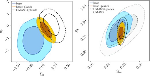
Constraints in the μ0−Σ0 plane (left), and Ωm−S8 plane (right) obtained from various combinations of the probes. The blue contours show the constraints obtained from the baseline case (DMASS 3 × 2 pt + CMASS RSD/BAO). The orange contours are obtained by adding the Planck data to the baseline case. The black-dashed contours are obtained from the external data only. The grey contour in the right panel shows the constraints of Ωm and S8 obtained from CMASS only. Adding the DMASS 3 × 2 pt data improves the constrains from the external data sets by 28 per cent for μ0, 30 per cent for Σ0, and 24 per cent for S8.
1D marginalized posteriors obtained from various combinations of data sets. ‘baseline’ denotes the combination of the DMASS 3 × 2 pt data and RSD and BAO measurements from BOSS CMASS.
| Data | μ0 | Σ0 | Ωm | σ8 | S8 | b |
|---|---|---|---|---|---|---|
| baseline | |$-1.23^{+0.81}_{-0.83}$| | |$-0.17^{+0.16}_{-0.15}$| | |$0.289^{+0.031}_{-0.028}$| | |$0.821^{+0.067}_{-0.068}$| | |$0.809^{+0.080}_{-0.079}$| | |$1.83^{+0.20}_{-0.17}$| |
| baseline + Planck | |$-0.37^{+0.47}_{-0.45}$| | |$0.078^{+0.078}_{-0.082}$| | |$\left(308.2^{+9.0}_{-8.0} \right) \times 10^{-3}$| | 0.762 ± 0.045 | |$0.772^{+0.050}_{-0.046}$| | |$2.134^{+0.079}_{-0.078}$| |
| DESY1 redMaGiC + CMASS + Planck | |$-0.29^{+0.63}_{-0.66}$| | |$0.098^{+0.102}_{-0.100}$| | (305.0 ± 8.6) × 10−3 | |$0.767^{+0.061}_{-0.065}$| | |$0.773^{+0.064}_{-0.067}$| | − |
| CMASS + Planck | |$0.15^{+0.61}_{-0.67}$| | |$0.20^{+0.12}_{-0.11}$| | |$0.314^{+0.012}_{-0.011}$| | |$0.794^{+0.057}_{-0.062}$| | |$0.814^{+0.059}_{-0.068}$| | |$2.00^{+0.28}_{-0.26}$| |
| CMASS | − | − | |$0.319^{+0.052}_{-0.055}$| | |$0.792^{+0.087}_{-0.084}$| | |$0.819^{+0.114}_{-0.119}$| | |$1.980^{+0.348}_{-0.313}$| |
Finally, we test the robustness of our results against unmodelled systematics. As shown in Fig. 3, the tangential shear signal measured with DMASS and the first source bin of DES Y1 is higher than predicted in theory. Lee et al. (2021) suggests the local peak in galaxy bias at the low-redshift end of the original BOSS CMASS sample as a potential reason for this. If the DMASS algorithm faithfully replicated the properties of CMASS, this peak would have been replicated in DMASS and even amplified at the low-redshifts edge where the algorithm poorly works. As the first source bin lies largely in front of the lens bin, it is possible that the tangential shear signal measured with the first source bin only captures correlations with the DMASS galaxies at low redshifts where galaxy bias peaks. Lee et al. (2021) tested the impact of the unmodelled local peak on the galaxy bias constraint inferred from the tangential shear measurement. In fixed ΛCDM cosmology, they found that the resulting constraint is not biased by the local peak above the scale of |$4 \, h^{-1}\, {\rm Mpc}$|. It is less likely that the local peak will affect our result as we utilize the scales larger than |$4 \, h^{-1}\, {\rm Mpc}$|, and include the angular galaxy clustering and shear measurements that are less sensitive to an irregularity in galaxy bias at the redshift tails. However, it is worth testing its impact in the frame of modified gravity as well to rule out the possibility of this unmodelled systematics biasing the result. For this, we repeat the analysis without the tangential shear signals from the first and second source bins. The signal from the second source bin is excluded to completely remove any potential effect related to galaxy bias from the low-redshift end of DMASS. The results are presented in Fig. 7. Each panel shows the contours of the MG parameters (left) and Ωm–S8 (right) with all tangential shear signals (solid lines) and without the signals from the first two source bins (dashed lines). Both panels are for the case of baseline + Planck. As shown in this figure, we do not find significant bias or degradation in the constraints.
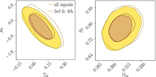
Constraints obtained with all four tomographic cross-correlations of γt (solid) and only with the third and fourth cross-correlations of γt (dashed) from the two highest source bins. All contours are the case of baseline + Planck. There is no significant bias or degradation found in the constraints.
7.2 Comparison with the DES Y1 MG analysis
Earlier, the DES Collaboration reported the constraints on μ0 and Σ0 obtained from the DES Y1 data in DESY1MG. As this work follows, their analysis methods with the same shear catalog, comparing the results of this work with DESY1MG enables us to validate the capability of using DMASS as gravitational lenses to combine the spectroscopic and imaging surveys efficiently. This section briefly describes the lens sample and external data sets used in DESY1MG and compares their MG constraints with ours. As we do not report the result for the DES data alone, we only compare the results measured with the external data sets.
DESY1MG utilized the 3 × 2 pt data vectors measured with the redMaGiC lenses (Rozo et al. 2016; Elvin-Poole et al. 2018) and the DES Y1 metacalibration sources (Sheldon & Huff 2017; Huff & Mandelbaum 2017; Zuntz et al. 2018). The redMaGiC sample consists of 660 000 galaxies over an area of |$1321\deg ^2$|. The sample was divided into five redshift bins, using three different cuts on intrinsic luminosity: 0.15 < z < 0.3, 0.3 < z < 0.45, 0.45 < z < 0.6, 0.6 < z < 0.75, and 0.75 < z < 0.9. The first three bins were selected using a luminosity cut of L > 0.5L* with a spatial density |$\bar{n} = 10^{-3} (\, h^{-1}\, {\rm Mpc})^{-3}$|, the other two bins were selected using L > L* with |$\bar{n}=4 \times 10^{-4} (\, h^{-1}\, {\rm Mpc})^{-3}$|, and L > 1.5L* with |$\bar{n}= 10^{-4} (\, h^{-1}\, {\rm Mpc})^{-3}$|, respectively. The redshift coverage of DMASS is comparable to the third and fourth bins of redMaGiC combined, but the number density of DMASS (|$\bar{n} = 3 \times 10^{-4}$|) is much lower than redMaGiC. The external data sets selected in DESY1MG were the CMB measurements from Planck 2015 (Planck Collaboration XII 2016), the RSD and BAO measurements from BOSS DR12 (Alam et al. 2017b), and the additional BAO measurements from Six-degree Field Galaxy Survey (6dF; Beutler et al. 2012), SDSS Main Galaxy Samples (SDSS MGS; Ross et al. 2015), and lastly, Type Ia supernova measurements from Pantheon (Scolnic et al. 2018). The resulting MG constraints from these data sets are |$\mu _0=-0.11^{+0.42}_{-0.46}$| and |$\Sigma _0=0.06^{+0.08}_{-0.07}$|.
For a more direct comparison with DESY1MG, we perform an additional analysis using DES Y1 3 × 2 pt (i.e. redMaGiC lenses) with CMASS RSD/BAO. By doing so, we can infer the pure improvement by DMASS while excluding contributions from other external data sets in DESY1MG. The resulting constraints of MG are |$\mu _0=-0.29^{+0.63}_{-0.66}$|, |$\Sigma _0=0.098^{+0.102}_{-0.100}$|.
Fig. 8 shows the constraints of this work (baseline + Planck) in orange, redMaGiC + CMASS RSD/BAO + Planck in purple, and DESY1MG in black-dashed lines. Compared to the case with redMaGiC (purple), it is noticeable that using DMASS (orange) improves the MG constraints by 29 per cent for μ0 and 21 per cent for Σ0 with the same external data sets despite redMaGiC consisting of five tomographic bins with a higher number density. Our result is also comparable to that of DESY1MG (black-dashed) despite the lack of the external data sets. This can be explained as follows: five tomographic bins of redMaGiC introduce additional nuisance parameters of galaxy bias for each bin. When combined with the CMASS likelihood, these five galaxy bias parameters from redMaGiC and an additional one from CMASS are varied independently, and hence uncertainties from the total six parameters add to the total statistical error budget. This especially affects the modified-gravity parameters due to the strong degeneracy among the galaxy bias and MG parameters. Compared with the other two cases, DESY1MG (black-dashed) slightly shifts towards a lower value of Ωm. The shift is possibly caused by the Pantheon supernova data that favors a relatively lower value of Ωm than the rest of the data sets (Scolnic et al. 2018). Overall, the constraints obtained with DMASS are consistent with those with redMaGiC. We do not find a significant shift in the central values of μ0 and Σ0 among the three cases.
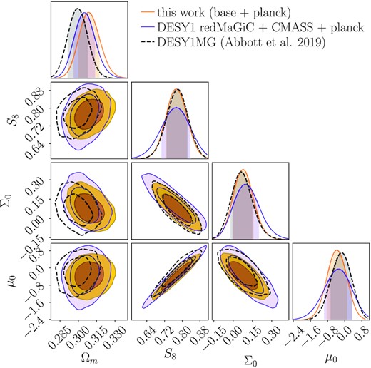
Constraints from this work (baseline + Planck; orange), DESY1 redMaGiC 3x2pt + CMASS RSD/BAO + Planck (purple), and the published constraints of the DES Y1 MG analysis (black-dashed) (Abbott et al. 2019). Compared to the case with redMaGiC (purple), using DMASS (orange) improves the MG constraints by 29 per cent for μ0 and 21 per cent for Σ0 with the same external data sets. The DMASS case is even comparable to that of DESY1MG (black-dashed) despite the lack of the external data sets. The shift of Ωm in DESY1MG is caused by the SNe Ia data favouring low Ωm. Overall, the constraints in the three cases are consistent.
8 CONCLUSION
In this paper, we measured the modified gravity parameters Σ0 and μ0 using the DMASS sample to demonstrate its feasibility as an equivalent to BOSS CMASS in the DES Y1 footprint for a joint analysis of BOSS and DES. We utilized the angular clustering of the DMASS galaxies, cosmic shear of the DES metacalibration sources, and cross-correlation of the two as data vectors. Then we derived the constraints on MG by jointly fitting the data vectors with the RSD and BAO measurements from the BOSS CMASS sample and CMB measurements from Planck. As detailed in Section 4, we thoroughly followed the analysis methods of DESY1MG. We employed the same modeling for the two-point statistics and potential systematics, such as the shear and photo-z biases. A series of tests were performed as done in DESY1MG to make sure our results are robust to the modeling assumptions that are not included in the pipeline.
The resulting constraints are consistent with GR. Adding DMASS 3 × 2 pt significantly improves the existing constraints from CMASS RSD/BAO + Planck by 28 per cent for μ0 and 30 per cent for Σ0. Not only that, we found that DMASS yields constraints improved by 29 per cent for μ0 and 21 per cent for Σ0, compared to the constraints obtained with redMaGiC when the same external data sets are utilized. The results are also comparable to the results of DESY1MG performed with additional BAO & RSD and supernova measurements. This is mainly because of a tightly constrained galaxy bias parameter shared in the CMASS and DMASS likelihoods, which breaks the degeneracy between galaxy bias and other parameters. Compared to that, the cases with redMaGiC treats the galaxy bias parameter from RSD as an additional one, which varies independently from those of redMaGiC. The uncertainty induced by the independent use of galaxy bias erases gains from additional BAO and RSD and supernova measurements.
This approach to optimally combine the DES and BOSS surveys with DMASS can be easily extended to other types of spectroscopic samples and image-based surveys. In just a few years, data from the Stage IV surveys will become available. The survey footprint of LSST7 (Ivezić et al. 2019) will occupy the entire southern sky with a small overlapping area with spectroscopic surveys such as DESI8 (DESI Collaboration 2016) in the northern sky. The DESI survey produces the Bright Galaxy sample (BGS) at z < 0.4 and the Emission Line Galaxy sample (ELG) at z > 0.6. The equivalent samples to those DESI targets in the LSST area will be ideal lenses to extract the lensing signals in LSST that can be efficiently combined with the galaxy clustering of the DESI galaxy samples as done with DMASS and CMASS. Combining the two surveys in this manner will embrace almost the entire sky and yield a wealth of information to test gravity.
SUPPORTING INFORMATION
Supplementary data are available at https://des.ncsa.illinois.edu/releases/other/y1-dmass.
Please note: Oxford University Press is not responsible for the content or functionality of any supporting materials supplied by the authors. Any queries (other than missing material) should be directed to the corresponding author for the article.
ACKNOWLEDGEMENTS
We thank D. H. Weinberg for useful conversations in the course of preparing this work.
AC acknowledges support from NASA grant no. 15-WFIRST15-0008. During the preparation of this paper, C.H. was supported by the Simons Foundation, NASA, and the U.S. Department of Energy.
The figures in this work are produced with plotting routines from matplotlib (Hunter 2007) and ChainConsumer (Hinton 2016). Some of the results in this paper have been derived using the healpy and healpix package (Górski et al. 2005; Zonca et al. 2019).
Funding for the DES Projects has been provided by the US Department of Energy, the US National Science Foundation, the Ministry of Science and Education of Spain, the Science and Technology Facilities Council of the United Kingdom, the Higher Education Funding Council for England, the National Center for Supercomputing Applications at the University of Illinois at Urbana-Champaign, the Kavli Institute of Cosmological Physics at the University of Chicago, the Center for Cosmology and Astro-Particle Physics at the Ohio State University, the Mitchell Institute for Fundamental Physics and Astronomy at Texas A&M University, Financiadora de Estudos e Projetos, Fundação Carlos Chagas Filho de Amparo à Pesquisa do Estado do Rio de Janeiro, Conselho Nacional de Desenvolvimento Científico e Tecnológico and the Ministério da Ciência, Tecnologia e Inovação, the Deutsche Forschungsgemeinschaft and the Collaborating Institutions in the Dark Energy Survey.
The Collaborating Institutions are Argonne National Laboratory, the University of California at Santa Cruz, the University of Cambridge, Centro de Investigaciones Energéticas, Medioambientales y Tecnológicas-Madrid, the University of Chicago, University College London, the DES-Brazil Consortium, the University of Edinburgh, the Eidgenössische Technische Hochschule (ETH) Zürich, Fermi National Accelerator Laboratory, the University of Illinois at Urbana-Champaign, the Institut de Ciències de l’Espai (IEEC/CSIC), the Institut de Física d’Altes Energies, Lawrence Berkeley National Laboratory, the Ludwig-Maximilians Universität München and the associated Excellence Cluster Universe, the University of Michigan, NFS’s NOIRLab, the University of Nottingham, The Ohio State University, the University of Pennsylvania, the University of Portsmouth, SLAC National Accelerator Laboratory, Stanford University, the University of Sussex, Texas A&M University, and the OzDES Membership Consortium.
Based in part on observations at Cerro Tololo Inter-American Observatory at NSF’s NOIRLab (NOIRLab Prop. ID 2012B-0001; PI: J. Frieman), which is managed by the Association of Universities for Research in Astronomy (AURA) under a cooperative agreement with the National Science Foundation.
The DES data management system is supported by the National Science Foundation under Grant Numbers AST-1138766 and AST-1536171. The DES participants from Spanish institutions are partially supported by MICINN under grants ESP2017-89838, PGC2018-094773, PGC2018-102021, SEV-2016-0588, SEV-2016-0597, and MDM-2015-0509, some of which include ERDF funds from the European Union. IFAE is partially funded by the CERCA program of the Generalitat de Catalunya. Research leading to these results has received funding from the European Research Council under the European Union’s Seventh Framework Program (FP7/2007-2013) including ERC grant agreements 240672, 291329, and 306478. We acknowledge support from the Brazilian Instituto Nacional de Ciência e Tecnologia (INCT) do e-Universo (CNPq grant no. 465376/2014-2).
This manuscript has been authored by Fermi Research Alliance, LLC under Contract No. DE-AC02-07CH11359 with the U.S. Department of Energy, Office of Science, Office of High Energy Physics.
Funding for SDSS-III has been provided by the Alfred P. Sloan Foundation, the Participating Institutions, the National Science Foundation, and the U.S. Department of Energy Office of Science. The SDSS-III web site is http://www.sdss3.org/.
SDSS-III is managed by the Astrophysical Research Consortium for the Participating Institutions of the SDSS-III Collaboration including the University of Arizona, the Brazilian Participation Group, Brookhaven National Laboratory, Carnegie Mellon University, University of Florida, the French Participation Group, the German Participation Group, Harvard University, the Instituto de Astrofisica de Canarias, the Michigan State/Notre Dame/JINA Participation Group, Johns Hopkins University, Lawrence Berkeley National Laboratory, Max Planck Institute for Astrophysics, Max Planck Institute for Extraterrestrial Physics, New Mexico State University, New York University, Ohio State University, Pennsylvania State University, University of Portsmouth, Princeton University, the Spanish Participation Group, University of Tokyo, University of Utah, Vanderbilt University, University of Virginia, University of Washington, and Yale University.
This work used resources at the Owens Cluster at the Ohio Supercomputer Center (OSC 1987) and the Duke Compute Cluster (DCC) at Duke University.
DATA AVAILABILITY
The DMASS galaxy catalogue used in this work and some of the ancillary data products shown in the Figures are available through the DES data release page (https://des.ncsa.illinois.edu/releases/other/y1-dmass). Readers interested in comparing to these results are encouraged to check out the release page or contact the corresponding author for additional information.
Footnotes
This statement about degeneracy assumes only linear scales, where MG can be modelled.
The DMASS sample does not cover the overlapping area between BOSS and DES since the sources from the area were used to train the DMASS algorithm. Thereby, the angular clustering and tangential shear signals used in this work are computed excluding the overlap. The shear measurement from Troxel et al. (2018) did not use the overlapping area as well.
As we do not have a pipeline to analyse the BOSS measurement of the two-point function directly, we had to rely on the cosmological inferences instead. Chuang et al. (2017) is the only published measurement of the BOSS CMASS galaxy clustering that provides the constraint on bσ8(z) and its covariance with other cosmological parameters. Future analyses using the same strategy will likely need to consider the full analysis of the two-point function to make use of the BAO reconstruction that is not included in Chuang et al. (2017).
Rubin Observatory’s Legacy Survey of Space and Time.
Dark Energy Spectroscopic Instrument.
