


ABSTRACT
We report here the discovery of a hot Jupiter at an orbital period of 3.208664 ± 0.000015 d around TOI-1789 (TYC 1962-00303-1, TESSmag = 9.1) based on the TESS photometry, ground-based photometry, and high-precision radial velocity (RV) observations. The high-precision RV observations were obtained from the high-resolution spectrographs, PARAS at Physical Research Laboratory (PRL), India, and TCES at Thüringer Landessternwarte Tautenburg (TLS), Germany, and the ground-based transit observations were obtained using the 0.43-m telescope at PRL with the Bessel-R filter. The host star is a slightly evolved (log g* = |$3.943^{+0.023}_{-0.043}$|), late F-type (Teff= 5991 ± 55 K), metal-rich star ([Fe/H] = |$0.373^{+0.071}_{-0.086}$| dex) with a radius of |$\, R_*$| = |$2.168^{+0.036}_{-0.034}$| R⊙ located at a distance of |$223.53^{+0.91}_{-0.90}$| pc. The simultaneous fitting of the multiple light curves and the RV data of TOI-1789 reveals that TOI-1789 b has a mass of |$\, M_{\rm P}$| = 0.70 ± 0.16 |$\, M_{\rm J}$|, a radius of |$\, R_{\rm P}$| = |$1.44^{+0.24}_{-0.14}$| |$\, R_{\rm J}$|, and a bulk density of ρP = |$0.28^{+0.14}_{-0.12}$| g cm−3 with an orbital separation of a = |$0.04882^{+0.00063}_{-0.0016}$| au. This puts TOI-1789 b in the category of inflated hot Jupiters. It is one of the few nearby evolved stars with a close-in planet. The detection of such systems will contribute to our understanding of mechanisms responsible for inflation in hot Jupiters and also provide an opportunity to understand the evolution of planets around stars leaving the main-sequence branch.
1 INTRODUCTION
Hot Jupiters have set several firsts, from being the first kind of exoplanets discovered with the radial velocity (RV) method (51 Peg; Mayor & Queloz 1995), to being also the first kind of transiting systems studied for precise radii and orbits (HD 209458 b; Charbonneau et al. 2000; Henry et al. 2000). These systems have intrigued the theorists triggering a critical revision of planet formation theories. Two theories have been used the most to explain close-in giant planets. These are the in situ formation by gravitational instability (Boss 1997; Durisen et al. 2007) or core accretion followed by inward migration (Perri & Cameron 1974; Chabrier et al. 2014). Gravitational instability envisions the formation of giant planets via the fragmentation of protoplanetary disc into bound clumps (Boss 1997). In the case of core accretion, the giant planet is formed at several astronomical units beyond the so-called ice-line where sufficient solid material is present to form the core, and then it migrates inward. The migration is caused by either torques from the protoplanetary disc or by gravitational scattering due to a third body. This can shrink the orbital separation of the planet from their formation location of several AUs to hundredths of AUs (Lin & Papaloizou 1986; Baruteau et al. 2014; Hamers & Tremaine 2017). One may refer Dawson & Johnson (2018) for a detailed review on the formation mechanism of hot Jupiters. Although a large number of close-in giant planets have been detected, this is largely a bias effect due to the ease in detecting them (high RV amplitude, short periods). The true frequency of close-in planets is only ∼ 1|${{\ \rm per\ cent}}$| (Johnson et al. 2010b; Mayor et al. 2011; Hsu et al. 2019, and references therein).
Space-based transit surveys like CoRoT (Baglin et al. 2006), Kepler (Borucki et al. 2010), and TESS (Ricker et al. 2015) have not only increased the number of discovered hot Jupiters, but their high photometric precision has allowed for the determination of the most precise planet radii and densities. These surveys have revealed that hot Jupiters tend to have inflated radii, typically |$10\!-\!50{{\ \rm per\ cent}}$| larger than that of Jupiter (Hartman et al. 2012; Espinoza et al. 2016; Raynard et al. 2018; Soto et al. 2018; Tilbrook et al. 2021). In some of the systems, heat is known to slow down the contraction of the planet (Showman & Guillot 2002; Komacek & Youdin 2017). Several mechanisms have been proposed to explain this inflation, one being star–planet tidal interactions (Bodenheimer, Laughlin & Lin 2003) and the other in which kinetic energy from the wind is converted into heat (Guillot & Showman 2002) and Ohmic dissipation (Batygin & Stevenson 2010). The most likely mechanism responsible for such inflation is the large incident stellar irradiation (Laughlin, Crismani & Adams 2011; Thorngren & Fortney 2018). However, this process alone is not enough to explain the inflation. It was suggested by Showman & Guillot (2002) that energy is dissipated by atmosphere circulation due to the transport of kinetic energy to the interior of planets which could additionally be contributing to the process of inflation (Baraffe et al. 2003). Evolved stars provide higher source of radiation due to their larger sizes compared to their solar analogues. There are only a handful of systems with giant stars harbouring planets interior to 0.5 au (eg. Lillo-Box et al. 2014; Jones et al. 2015; Ortiz et al. 2015). Thus, it is imperative to look at stars which might be leaving the main sequence phase and entering the sub-giant/giant branch. It is interesting to catch these stars in an evolutionary phase that has yet not caused the engulfment of its orbiting planet. There have been only a handful of such close-in planets discovered as of now orbiting around slightly evolved stars, e.g. KELT-12 b (Stevens et al. 2017) and TOI-640 b (Rodriguez et al. 2021) to name a few.
In this paper, we present the discovery of a hot Jupiter around a star TYC 1962-00303-1 or TESS Object of Interest TOI-1789, an important contribution to this field of relatively rare kinds of planets around slightly evolved stars. We use spectroscopic, photometric, and imaging data to confirm the nature of this transiting candidate and to characterize the planet in terms of its mass, radius and density. All the observations are described in Section 2 of the paper. In Section 3, we focus on the host star and characterization of the star–planet system in detail with the joint modeling of transit photometry and RVs. In Section 4, we discuss the implications of our results with summarizing the paper in Section 5.
2 OBSERVATIONS
2.1 TESS photometry
TYC 1962-00303-1 is a relatively bright star (V = 9.7 mag) in the northern celestial hemisphere, first listed as TOI-1789 on 2020 March 12. This source was observed by TESS between 2020 January 21 and February 18 (27.3-d time-span) with a gap of ∼2 d due to the data transferring from the spacecraft. TESS operates at a wavelength region of 600–1000 nm and covers 21arcsec of sky in each pixel (Ricker et al. 2015). It has four identical cameras with a 24 × 24 deg2 field of view for each camera. TOI-1789 was observed in the CCD-4 of camera 1 in sector 21 in a long cadence (30 min) mode.
The data were analyzed with the Quick Look Pipeline (QLP: Huang et al. 2020) developed by MIT and the Science Processing Operations Center (SPOC: Jenkins et al. 2016) pipeline, based on the Kepler mission pipeline at the NASA Ames research centre. Both pipelines detected eight transits with a depth of ∼2600 ppm for TOI-1789 spaced at a period of ∼ 3.21 d and a duration of ∼ 2.3 h. The transit data is also vetted by the TESS Science team before releasing it as a planetary candidate. The transits are reported to be V-shaped and a slight centroid offset in the target position. We adopt the Pre-search Data Conditioning Simple Aperture Photometry (PDCSAP) light curves (LC; Smith et al. 2012; Stumpe et al. 2014), provided by the SPOC pipeline, which is publically available at the Mikulski Archive for Space Telescopes (MAST).1 We applied the Box Least Square (BLS; Kovács, Zucker & Mazeh 2002) periodogram to detect the transits in the TESS LC using PDCSAP fluxes. We successfully retrieved the transit signal at a period of 3.207 6208 with a depth of 2610 ± 220 ppm. To search for additional transit signals, we removed this 3.207 6208-d signal from the data and re-ran the BLS periodogram. We did not find any other significant peaks. For further analysis, we use median-normalized PDCSAP fluxes that are additionally detrended by fitting a high-order polynomial over out-of-transit data using the lightkurve package (Lightkurve Collaboration et al. 2018). The basic properties of the star found in the literature are listed in Table 1.
Basic Stellar Parameters for TOI-1789.
| Parameter | Description (unit) | Value | Source |
|---|---|---|---|
| αJ2000 | Right Ascension | 09 30 58.42 | (1) |
| δJ2000 | Declination | 26 32 23.98 | (1) |
| μα | PM in RA (mas yr−1) | −7.977 ± 0.019 | (1) |
| μδ | PM in Dec. (mas yr−1) | −39.401 ± 0.015 | (1) |
| |$\pi$| | Parallax (mas) | 4.474 ± 0.0181 | (1) |
| G | Gaia G mag | 9.584 ± 0.0002 | (1) |
| T | TESS T mag | 9.182 ± 0.006 | (2) |
| BT | Tycho B mag | 10.422 ± 0.039 | (3) |
| VT | Tycho V mag | 9.788 ± 0.031 | (3) |
| B | APASS B-mag | 10.335 ± 0.020 | (6) |
| V | APASS V-mag | 9.686 ± 0.030 | (6) |
| g | SDSSg mag | 10.353 ± 0.100 | (6) |
| r | SDSSr mag | 9.590 ± 0.060 | (6) |
| i | SDSSi mag | 9.398 ± 0.020 | (6) |
| J | 2MASS J mag | 8.672 ± 0.024 | (4) |
| H | 2MASS H mag | 8.410 ± 0.021 | (4) |
| KS | 2MASS KS mag | 8.345 ± 0.018 | (4) |
| W1 | WISE1 mag | 8.297 ± 0.023 | (5) |
| W2 | WISE2 mag | 8.348 ± 0.02 | (5) |
| W3 | WISE3 mag | 8.311 ± 0.024 | (5) |
| W4 | WISE4 mag | 7.996 ± 0.226 | (5) |
| Other Identifiers: | |||
| HD 82139 (7) | |||
| TIC 172518755 (2) | |||
| TYC 1962-00303-1 (3) | |||
| 2MASS J09305841 + 2632246 (4) | |||
| GaiaEDR3 646125297938578944 (1) | |||
References – (1) Gaia Collaboration et al. (2021), (2) Stassun et al. (2018), (3) Høg et al. (2000), (4) Cutri et al. (2003), (5) Cutri et al. (2021), (6) Henden et al. (2016), and (7) Cannon & Pickering (1993).
Notes. The spectral type for TOI-1789 reported by SIMBAD is K0, however, with our spectral analysis we find it to be a late F-type star (see Section 3.1.1 and 4.1).
The system is reported to be a widely separated visual binary with the secondary star TYC 1962-475-1 of similar spectral type and brightness (see Fig. 1), and with an orbital separation of 17776 AU (1.3-arcmin separation on the sky) (Andrews, Chanamé & Agüeros 2017). The Renormalized Unit Weight Error (RUWE) number from the Gaia catalogue for the target star is 0.948, a value ∼ 1, indicative that a single-star model is used as the best fit for astrometric observations (Gaia Collaboration et al. 2021). RUWE > 1.4 could indicate a binary nature for the astrometric solution used in Gaia. The on-sky separation for these two sources is larger than the TESS pixel scale of 21 arcsec.
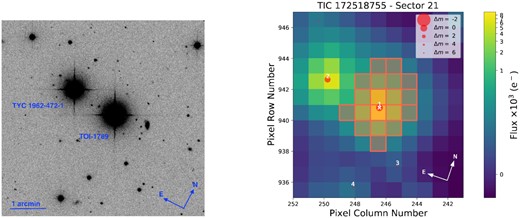
Left-hand panel: The SDSS (DR7) image of TOI-1789 and its visual binary companion (TYC 1962-472-1) in sloan-i band2. Right-hand panel: Target pixel file (TPF) of TOI-1789 in TESS sector 21 generated with tpfplotter (Aller et al. 2020). The sizes of individual red dots represent the magnitude contrast (Δm) with TOI-1789. The red-squared region represents the aperture used for photometry by SPOC and the position of TOI-1789 and TYC 1962-472-1 is labelled ‘1’ and ‘2’, respectively.
Based on the Kepler manual (Thompson et al. 2016), these PDCSAP fluxes are corrected for any contamination from neighbouring pixels. However, due to the V-shape, short transit duration (∼ 2 h), and the long cadence data (30 min), the transit shape, transit duration, and the planetary radius can not be determined precisely. There is also a small centroid offset in the target’s position given in the TESS data validation report. We, therefore, conducted short-cadence (∼ 20 s) ground-based transit observations to precisely obtain the transit parameters and to understand and verify the nature of the transits detected by TESS (see Section 2.2).
2.2 Ground-based photometry
We acquired ground-based transit follow-up observations for TOI-1789 with the 0.43-m telescope (CDK17 from PLANEWAVE)3 located at Gurushikhar Observatory, PRL, Mt. Abu, India. Five transits were observed between 2021 January 8 and March 10, as summarized in Table 2. The first three transits were observed using a low-cost TRIUS PRO-814 (TRI) CCD4, which provides a field of view (FOV) of 14.6 × 11.7arcmin2 with a pixel scale of 0.26 arcsec. For the last two transits an ANDOR iKon-L 936 (ADR) CCD5 was used, which has an FOV of 32 × 32 arcmin2 with a pixel scale of 0.95 arcsec. The telescope was slightly defocused while observing these events to have longer exposure times, which resulted in high-signal-to-noise ratio (S/N) and thus, helped in achieving higher photometric precision. All the transits were observed in the Bessel-R passband and the main specifications of both the CCDs are listed in Table 3. The use of ANDOR iKon-L 936 CCD in precision differential photometric observations is well established as the same kind of CCD detectors are used in various transit surveys like the SuperWASP (Pollacco et al. 2006) and the SPECULOOS (Sebastian et al. 2020). We used the AstroImageJ software (AIJ: Collins et al. 2017) for data reduction and LC extraction. AIJ is an efficient tool for time-series ultraprecise differential photometry (e.g. exoplanet transits), LC detrending, fitting, and plotting. First, the raw science frames were dark-corrected and flat fielded. Then, for the LC extraction, we did the multi-aperture differential photometry, as described in the Collins et al. (2017). An aperture of 1.5 times the FWHM of the star is used. The extracted LCs for all the five transit observations were detrended with respect to FWHM, airmass, and exposure time. These parameters are linearly detrended and their contribution is added to the overall χ2 contribution for the curve fitting within AIJ for each transit (see equation 5 in Collins et al. 2017). Finally, the normalized LCs were extracted from AIJ. The transit event was clearly visible in all the detrended LCs, as shown in Fig. 2. For better display purpose, we have binned the LC to 20 min. All the transits were jointly modelled with the observed RV data (Section 3.3.2). The residuals from the best-fitting transit model have a standard deviation of 1.16 ppt [parts per thousand, (∼ 1.3 mmag)] and 0.92 ppt (∼ 1 mmag) in 5 min bins for TRI and ADR data sets, respectively. The precision achieved with TRIUS CCD camera is within the 1.3σ of the precision achieved with ANDOR CCD camera showing that the low-cost CCD camera like TRIUS PRO-814 can also be used for precision differential photometric observations effectively.

Upper panel: The normalized TESS LC of TOI-1789 is plotted in red. Eight transits can be seen spaced at ∼3.21 d with a depth of ∼2.6 ppt. Middle panel: The ground-based follow-up photometry with PRL 0.43-m telescope is shown here (Section 2.2). The blue dots represent the three transits observed with a TRIUS CCD (TRI) with a precision of 1.16 ppt (∼ 1.3 mmag), while green dots represent the two transit events observed with an ANDOR CCD (ADR) with a precision of 0.92 ppt (∼ 1 mmag) in 5-min bins. Lower left-hand panel: All the transits identified by the CCD detector are phased to the orbital period of TOI-1789 b and then binned to 5- and 20-min cadence are plotted here, with blue and green colour depicting the TRI and ADR data sets, respectively. Lower right-hand panel: Red dots represent the phase folded TESS LC (30-min cadence). Note: In all the panels, the overplotted black line represents the best-fitting transit model from EXOFASTv2, obtained by simultaneous fitting of TESS and PRL photometry data (for details, refer Section 3.3.2).
A summary of the ground-based transit follow-up observations.
| Instrument | UT Date | Coverage | 5-min Precision (ppt) | Average PSF (arcsec) | Average EXP-TIME |
|---|---|---|---|---|---|
| TRIUS PRO-814 | 08 Jan 2021 | Full | 0.94 | 4.1 | 25s |
| TRIUS PRO-814 | 21 Jan 2021 | Full | 1.04 | 4.4 | 25s |
| TRIUS PRO-814 | 06 Feb 2021 | Full | 1.32 | 3.9 | 20s |
| ANDOR iKon-L 936 | 07 Mar 2021 | Full | 0.89 | 6.2 | 18s |
| ANDOR iKon-L 936 | 10 Mar 2021 | Full | 1.00 | 4.5 | 8s |
Specifications of both the CCDs.
| Specifications | TRIUS PRO-814 | ANDOR iKon-L 936 |
|---|---|---|
| Manufacturer | Starlight Xpress Ltd. | Oxford Instruments |
| Sensor type | Monochrome ICX814AL | e2V CCD42-40 |
| (Interline CCD) | (BEX2-DD) | |
| Image format (pix) | 3388 x 2712 | 2048 x 2048 |
| Pixel size (μm) | 3.69 | 13.5 |
| QE (at 580 nm) | ∼ 77% | |$\ge 90\%$| |
| Dark current (e−/s/pix) | ≤ 0.002 at −10°C | 0.006 at −80°C |
| System gain (e−/ADU) | 0.25 | 1 |
| Readnoise | 3e− at 3 MHz | 7e− at 1 MHz |
2.3 High-resolution speckle imaging
High-resolution imaging is a tremendously useful tool for finding contamination from nearby star. TOI-1789 was observed on 2021 February 3 ut using the ‘Alopeke speckle instrument on the Gemini North 8-m telescope6. ‘Alopeke provides simultaneous speckle imaging in two bands (562 and 832 nm) with output data products including a reconstructed image with robust contrast limits on companion detections (e.g. Howell et al. 2016). Five sets of 1000 × 0.06 s exposures were collected and subjected to Fourier analysis in the standard reduction pipeline (see Howell et al. 2011). If a nearby companion star is present, interferometric fringes are detected in the Fourier analysis and used to determine the companion separation, position angle, and magnitude contrast (Δm). Fig. 3 shows our final 5σ contrast curves and reconstructed speckle images. The mean value of each reconstructed image is determined and then radial annuli are made in which each pixel is determined to be above or below the mean. The accumulation of such radial values is used to fit a polynomial curve at a 5σ contrast level resulting in the two curves shown in Fig. 3. We do not find any companion brighter than Δm ∼ 5 within |$1.17$| arcsec of the target. At the distance of TOI-1789 (d = 223 pc), these angular limits correspond to spatial limits of upto 268 AU.
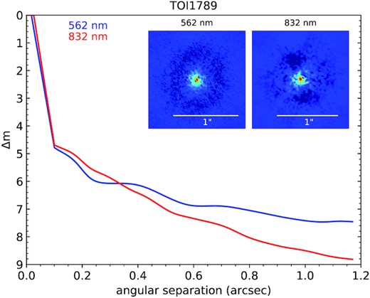
Gemini observations of TOI-1789 on ut 2021 February 3. The 5σ contrast curves are plotted with their reconstructed images.
2.4 Spectroscopy
The mass of the planet is determined by precise RV measurements made from the spectrographs PARAS and TCES configured at relatively small aperture-sized telescopes (1–2 m) located, respectively, at Mount Abu, Physical Research Laboratory (PRL), India, and Thüringer Landessternwarte Tautenburg (TLS), Germany. We describe these observations in the follwing sub-sections.
2.4.1 PARAS-PRL
We acquired a total of 16 spectra of TOI-1789 with the PARAS spectrograph (Chakraborty et al. 2014) attached to the PRL 1.2-m telescope at the Gurushikhar observatory, Mt. Abu, India. PARAS is a high-resolution (R ∼ 67000), fiber-fed, pressure and temperature stabilized echelle spectrograph, working in the wavelength range of 380 to 690 nm for precise RV measurements. These spectra were obtained between 2020 December 19 and 2021 March 19 using the simultaneous wavelength calibration mode either with Thorium-Argon (ThAr) or with Uranium-Argon (UAr) hollow cathode lamp (HCL) as described in Chakraborty et al. (2014) and Sharma & Chakraborty (2021), respectively. Only one among the 16 stellar spectra from PARAS was acquired with ThAr HCL, and that was observed on December 19, 2021. After that due to unavailability of pure-Th HCL, we switched to UAr HCL, and the remaining data were acquired with the UAr HCL.
The exposure time for each observation was kept at 1800 s, which resulted in an S/N per pixel of 12 to 20 at the blaze wavelength of 550 nm. The data reduction were carried out by an automated custom-designed pipeline written in IDL, that is based on the algorithms of Piskunov & Valenti (2002). The extracted spectra through this reduction procedure is further used for RV measurements. The RVs were determined by cross-correlating the stellar spectra with a numerical stellar template mask of the same spectral type (Baranne et al. 1996). For more details about PARAS data reduction, analysis pipeline, and RV precision stability of the instrument see Chakraborty et al. (2014, 2018). The offset between absolute RVs derived using ThAr and UAr spectra is found to be 10 m s−1, calculated using a standard RV star HD55575 (Sharma & Chakraborty 2021), and that has been corrected in TOI-1789 RVs for further analysis. All the RVs from PARAS are listed in Table 5 along with its respective errors. The errors reported here are based on the fitting errors of cross-correlation function (CCF) and the photon noise, calculated in the same way, as described in Chaturvedi et al. (2016, 2018).
2.4.2 TCES-TLS
A total of 21 useful spectra were obtained with the Tautenburg coude echelle spectrograph (TCES) installed at the 2-m Alfred Jensh telescope at the Thüringer Landessternwarte Tautenburg, Germany between 2021 February 22 and 2021 April 05. TCES is a slit spectrograph with a resolving power of R = 67 000 and a wavelength coverage of 470–740 nm. The spectrograph is installed in a Coude room with a temperature stabilized environment. For details of the observations, one can refer to Guenther et al. (2009). The iodine cell, inserted in the optical path of the spectrograph, acts as a wavelength reference for the spectra. The exposure time for all the obtained spectra were 1800 s each leading to an average S/N per pixel of ∼ 43 at 564 nm. The standard IRAF routines were used for data reduction that subtract the bias, flat-field the spectra, remove the scattered light, and extract the spectra. A first-order wavelength calibration is applied through Thorium–Argon calibration lamp, which is taken in the beginning and end of each night. Instantaneous wavelength solution is determined by the superimposed iodine lines. The iodine absorption cell technique requires a complex forward modelling procedure to estimate the Doppler shift in the stellar absorption lines. This technique is instrument specific and depends on the PSF of the spectrograph (Valenti, Butler & Marcy 1995). RVs are computed by a Python-based software Velocity and Instrument Profile EstimatoR (viper)7 (Zechmeister, Köhler & Chamarthi 2021), which is currently being developed as an open-source and a common approach for instrument profile and RV estimation using the Iodine technique. It is based on the standard procedure as described in Butler et al. (1996) and Endl, Kürster & Els (2000).
3 ANALYSIS AND RESULTS
To derive the stellar and planetary properties of TOI-1789 system, we analyzed our photometric and spectroscopic observations in the following subsections. Here, we give a brief summary of the procedure and present our results.
3.1 The host star
3.1.1 Spectroscopic parameters
We determine the spectroscopic parameters by using a relatively high S/N (∼ 65 per pixel) spectrum taken without the iodine cell at TCES-TLS. As a first step, we applied the empirical software SpecMatch-Emp code (Hirano et al. 2018) that compares well-characterized FGKM stars observed with Keck/HIRES to the data, in our case, the TCES-TLS spectra with R = 67 000. We obtain a stellar effective temperature, Teff = 5804 ± 110 K, a stellar radius, R* = 2.078 ± 0.180R⊙, and the abundance of the key species iron relative to hydrogen, [Fe/H] = 0.29 ± 0.09 (dex) as mentioned in Table 4. To perform a more detailed model, we used the spectral analysis package SME (Spectroscopy Made Easy; Valenti & Piskunov 1996; Piskunov & Valenti 2017) version 5.22. This code is based on grids of recalculated stellar atmospheric models that calculates a synthetic spectrum. The best-fitted stellar parameters are derived through a χ2 −minimization iteration that compares the synthetic and observed spectra for a given set of parameters. The spectra was synthesised based on the atomic and molecular line data from VALD (Ryabchikova et al. 2015) and the Atlas12 (Kurucz 2013) atmosphere grids. We refer to Fridlund et al. (2017) and Persson et al. (2018) for a more detailed description of the modelling. Briefly, we chose to model spectral features sensitive to different photospheric parameters: Teff from the Hα line wings, and the surface gravity, log g*, from the Ca i λλ6102, 6122, and 6162 triplet, and the λ6439 line. The abundances of iron and calcium, and the projected stellar rotational velocity, v sin i were fitted from narrow, unblended lines between 6100 and 6500 Å. We derive the vsin i as 7.0 ± 0.5 km s−1. We fixed the micro- and macro-turbulent velocities, Vmic and Vmac, to 1 and 3 km s−1 (Bruntt et al. 2010; Doyle et al. 2014), respectively. The results from SME are in good agreement within the uncertainties with SpecMatch-Emp (Table 4). The SME derived stellar parameters are supplied as priors in the global modelling. The finally adopted stellar parameters obtained through global modelling of the RV and transit data are indicated in the last row of Table 4 in bold font. For more details on the global modelling, see Section 3.3.2. One thing to note here is that we find the TOI-1789 is a late F-type star with our spectral analysis. Nevertheless, SIMBAD reported it as ‘K0’ spectral type.
Spectroscopic Properties derived for TOI-1789.
| Spectroscopic parameters | Teff | [Fe/H] | log g* |
|---|---|---|---|
| (K) | (dex) | (dex) | |
| SME | 5894 ± 142 | 0.38 ± 0.1 | 4.2 ± 0.2 |
| SpecMatch-Emp | 5804 ± 110 | 0.29 ± 0.09 | – |
| Global modelling | |$5984^{+55}_{-57}$| | |$0.370^{+0.073}_{-0.089}$| | |$3.939^{+0.024}_{-0.046}$| |
| Spectroscopic parameters | Teff | [Fe/H] | log g* |
|---|---|---|---|
| (K) | (dex) | (dex) | |
| SME | 5894 ± 142 | 0.38 ± 0.1 | 4.2 ± 0.2 |
| SpecMatch-Emp | 5804 ± 110 | 0.29 ± 0.09 | – |
| Global modelling | |$5984^{+55}_{-57}$| | |$0.370^{+0.073}_{-0.089}$| | |$3.939^{+0.024}_{-0.046}$| |
3.1.2 Rotational period determination
TOI-1789 is a moderately rotating star as determined through SME spectral modelling for vsin i of 7.0 ± 0.5 km s−1. We use the radius of |$2.168^{+0.036}_{-0.034}$| R⊙ (from global modelling Section. 3.3) to calculate the rotational period of about 15.7 d by assuming that the star is observed equator-on (i = 90°). Due to the presence of active regions or spots on the surface of the star, the rotation of the star often produces a non-sinusoidal signal. The lifetime of these signals is not well constrained and the differential rotation of the star makes this signal quasi-periodic (Dumusque et al. 2011; Haywood et al. 2014). These activity-induced signals are also introduced in the RV data, making it a nuisance for the planet detection. Such activity signals often cannot be modelled through a plain sinusoidal function. The non-parametric Gaussian processes can be used to model these signals (Angus et al. 2018).

Histogram for the posterior distribution function (PDF) for the estimated rotational period of the star (Period) while using the combined and nightly binned photometric data sets from ASAS, SuperWASP, KELT. We see the PDF peaking at 16 d with other less significant peaks at 8 and 32 d.
3.1.3 Bisector analysis
To investigate the cause of the RV variations in the PARAS data, we did the bisector analysis. The bisectors are calculated from the PARAS CCFs, where the CCF represents the average profile of the lines in the stellar mask used to calculate RVs. As described in Martínez Fiorenzano et al. (2005), we calculate the bisector of each horizontal segment of the CCF, which are at the same flux level from left to right. The line bisector is the combination of all these bisectors from the core to the wings of the CCF. Then the bisector velocity span (BIS) is calculated by taking the difference of average velocity values between the top and bottom zones of the CCF (BIS = Vtop – Vbottom). This difference (BIS) represents the symmetry of the CCF or the absorption lines in the spectra. A strong correlation, negative or positive, between RVs and BIS corresponds to the RV signal being attributed to stellar activity caused by spots or by other atmospheric phenomena like granulation, pulsation or turbulence, or due to likely contamination in the spectra from a nearby star (Queloz et al. 2001; Martínez Fiorenzano et al. 2005).
As described in Section 2, RV data are in phase with the transit ephemeris. From Section 3.1.2, the estimated rotation period is between 15-16 d a value much different than the planet period of 3.21 d. As it can be seen in Fig. 5, we do not find any significant correlation (Correlation coefficient ≈ 0.15, p-value = 0.58). Thus, activity related correlation seems unlikely. Moreover, we do not see any likely contamination of the target star from high-resolution imaging and neither any signature of blending in the bisector analysis. Thus, we conclude that the RV variations are due to the planetary signature seen in the data. The values for RVs, BVS and their respective error bars are listed in Table 5, and the BVS plotted against RVs are shown in Fig. 5.

Plot of bisector analysis from PARAS data. No significant correlation was observed between RV and BIS (correlation coefficient ≈ 0.15, p-value = 0.58).
RV measurements for TOI-1789. The BJDTDB is mentioned in the first column followed by their corresponding relative RVs and error in RVs in the second and third column, respectively. The fourth and fifth columns correspond to BIS and its respective errors. The sixth column represents the exposure time and the last column shows the instruments used for observations.
| BJDTDB | Relative-RV | σ-RV | BIS | σ-BIS | EXP-TIME | Instrument |
|---|---|---|---|---|---|---|
| (d) | (m s−1) | (m s−1) | (m s−1) | (m s−1) | (s) | |
| 2459203.519645 | −11.91 | 30.00 | 197.79 | 168.29 | 1800 | PARASa |
| 2459236.471110 | -91.76 | 28.13 | 267.54 | 64.79 | 1800 | PARASb |
| 2459236.495532 | −106.14 | 31.24 | 307.58 | 58.14 | 1800 | PARASb |
| 2459264.241224 | −34.16 | 26.40 | 972.78 | 93.32 | 1800 | PARASb |
| 2459264.426243 | −53.28 | 38.74 | -83.81 | 79.54 | 1800 | PARASb |
| 2459266.309799 | −98.94 | 46.13 | 1751.67 | 220.13 | 1800 | PARASb |
| 2459287.283471 | −44.48 | 20.80 | −551.95 | 30.95 | 1800 | PARASb |
| 2459289.186833 | −125.73 | 46.89 | −982.45 | 153.12 | 1800 | PARASb |
| 2459289.258414 | −100.47 | 23.03 | −100.73 | 87.37 | 1800 | PARASb |
| 2459289.284072 | −87.48 | 22.52 | 0.70 | 36.28 | 1800 | PARASb |
| 2459289.324973 | −134.37 | 23.88 | −415.21 | 28.96 | 1800 | PARASb |
| 2459290.195198 | −31.61 | 25.76 | 175.88 | 36.30 | 1800 | PARASb |
| 2459292.327774 | −26.77 | 31.32 | 86.37 | 59.11 | 1800 | PARASb |
| 2459293.265260 | −38.99 | 25.86 | −52.63 | 26.21 | 1800 | PARASb |
| 2459293.288928 | 16.25 | 28.94 | −80.99 | 101.90 | 1800 | PARASb |
| 2459293.336772 | −68.44 | 33.08 | −79.96 | 90.14 | 1800 | PARASb |
| 2459268.367086 | 55.72 | 30.32 | – | – | 1800 | TCES |
| 2459269.344931 | 4.01 | 28.88 | – | – | 1800 | TCES |
| 2459270.328739 | 211.94 | 31.26 | – | – | 1800 | TCES |
| 2459276.311054 | 142.06 | 37.66 | – | – | 1800 | TCES |
| 2459277.276355 | 133.96 | 37.06 | – | – | 1800 | TCES |
| 2459277.413716 | 115.03 | 32.70 | – | – | 1800 | TCES |
| 2459297.373577 | 42.26 | 14.10 | – | – | 1800 | TCES |
| 2459298.323521 | −25.34 | 14.19 | – | – | 1800 | TCES |
| 2459297.462606 | 136.68 | 39.96 | – | – | 1800 | TCES |
| 2459298.451947 | 61.38 | 20.11 | – | – | 1800 | TCES |
| 2459299.393539 | 292.36 | 31.03 | – | – | 1800 | TCES |
| 2459300.315441 | 151.34 | 29.86 | – | – | 1800 | TCES |
| 2459303.279352 | 179.31 | 34.34 | – | – | 1800 | TCES |
| 2459303.300500 | 187.65 | 33.82 | – | – | 1800 | TCES |
| 2459303.436010 | 142.56 | 26.32 | – | – | 1800 | TCES |
| 2459303.457166 | 205.70 | 23.46 | – | – | 1800 | TCES |
| 2459305.274017 | 128.12 | 24.60 | – | – | 1800 | TCES |
| 2459305.295176 | 101.73 | 29.09 | – | – | 1800 | TCES |
| 2459309.278728 | 281.19 | 30.41 | – | – | 1800 | TCES |
| 2459309.300456 | 226.44 | 27.72 | – | – | 1800 | TCES |
| 2459310.422304 | 113.38 | 38.13 | – | – | 1800 | TCES |
Spectra acquired simultaneously with ThAr HCL.
Spectra acquired simultaneously with UAr HCL.
3.2 Periodogram analysis
We show the computed Generalized Lomb–Scargle periodogram (GLS; Zechmeister & Kürster 2009) for RVs, residual RVs, window function, FWHM, and BIS in Panels 1–5 (top to bottom) in the Fig. 6, respectively. For finding the periodicities in our RV data, we combined RVs from both the spectrographs, PARAS and TCES. First, we corrected the instrumental offsets from RVs by subtracting corresponding average RV values and then computed the periodogram (Panel 1). Here, we use the equations given in Zechmeister & Kürster (2009) to normalize the periodogram and calculate false alarm probability (FAP). We consider the threshold FAP of 0.1 per cent for any significant signal and find the most significant signal at a period of ∼ 3.21 d (marked as vertical dashed line in Fig. 6), the same as the orbital period derived from the transit data (both ground and space-based) for this planetary candidate. We evaluated the FAP at this periodicity using a bootstrap method of 1000 000 randomization, over a very narrow range, centring at this period. It gives an FAP of 0.007 per cent, which strongly confirms a periodic signal in our RV data set. There are other two significant signals in the RV periodogram at a period of ∼ 0.76 and 1.45 d that vanish when we subtract this ∼ 3.21-d periodic signal using a best-fitting sinusoidal curve, as can be seen in the residual periodogram (Panel 2). These are the 1-d aliases of the orbital frequency (forb) or the 3.21-d signal. Specifically, 1/0.76 is the 1-d alias of forb, and 1/1.45 is the 1-d alias of –forb. The residual periodogram does not show any other significant periodicity with FAPs above our threshold of 0.1 per cent. The spectral window function is shown in the Panel 3. Furthermore, we also computed the GLS periodogram of the CCF FWHMs and BIS using PARAS data, which is shown in Panels 4 and 5, respectively (for more information of bisector analysis, please see Section 3.1.3). These diagnostics are generally used as stellar activity indicators since they quantify the line asymmetries which mimic the Doppler shifts. We do not find any statistical significant signals of the stellar activity in the periodograms. Here, we could not use the TCES data as it has superimposed iodine lines in the spectra.
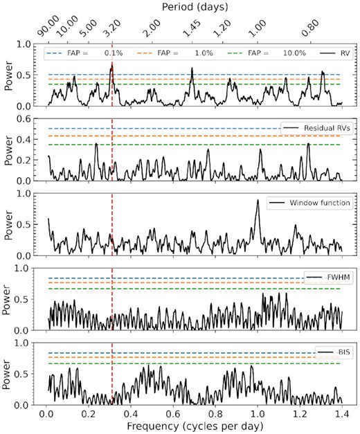
The GLS periodogram for the RVs, residual RVs, window function, FWHM, and bisector span of TOI-1789 is shown in Panels 1–5 (upper to lower) respectively. The primary peak is seen at a period ≈3.21 d (dashed red line), consistent with the orbital period of the planetary candidate obtained from photometry. The FAP levels (dashed lines) of 0.1, 1, and 10 |${{\ \rm per\ cent}}$| for the periodograms are shown in the legends in the panel 4. Note. For periodogram analysis of the RVs, the whole data set was used. In contrast, only PARAS data was used for the last two analyses as superimposed iodine lines are presented in TCES spectra.
3.3 Global modelling
We used EXOFASTv2 (Eastman et al. 2019) to constrain the host star parameters in the global model and find the orbital and planetary parameters of the system. The EXOFASTv2 uses the Differential Evolution Markov Chain Monte Carlo (MCMC) technique to fit the multiplanetary systems with multiple RV and photometry datasets and at the same time provides the opportunity for deriving stellar parameters using spectral energy distribution (SED) and isochrones. It also diagnoses the convergence of the chains using built-in Gelman–Rubin statistics (Gelman & Rubin 1992; Ford 2006).
3.3.1 Modelling the host star
We derive the host star parameters using the MIST isochrones (Choi et al. 2016; Dotter 2016) and the Spectral Energy Distribution (SED) fitting (Stassun & Torres 2016) using the Kurucz stellar atmosphere model (Kurucz 1979) within the EXOFASTv2 framework. The SED fitting combined with MIST isochrones and transit precisely determine the mass, radius, log g*, and age of the star (Torres, Winn & Holman 2008). Therefore, we use the TESS and ground-based transit data to constrain the stellar parameters. We place Gaussian priors on Teff and [Fe/H], derived from the spectral analysis, and parallax from GaiaEDR3 (Gaia Collaboration et al. 2021). A uniform prior with an upper limit on V-band extinction from the Schlafly & Finkbeiner (2011) and dust maps at the location of the host star are also applied. We plot the log g* versus Teff corresponding to Table 6 in Fig. 7 and show the most likely MIST evolutionary track for TOI-1789 (solid line). We also show the evolutionary tracks (dashed lines) of two different masses 1.36 and 1.64 M⊙ (± 0.14 of the mass of TOI-1789) in the figure. We used broadband photometry from Tycho BV (Høg et al. 2000), APASS DR9 BV, SDSSgri (Henden et al. 2016), 2MASS JHK (Cutri et al. 2003), ALL-WISE W1, W2, W3, and W4 (Cutri et al. 2021), which are listed in Table 1. The best-fitted SED model along with these broadband photometry fluxes are shown in Fig. 8.
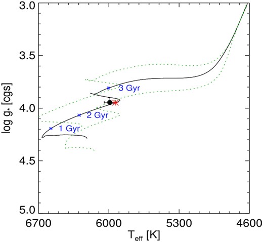
The solid black line depicts the most likely evolutionary track for TOI-1789 from MIST. The black circle is at the model value Teff and log g* with its errorbars. The red asterisk represents the model value for equal evolutionary point (EEP) or the age of TOI-1789 along the track. The other two dashed lines are the evolutionary tracks of masses 1.36 and 1.64 M⊙, whereas blue asterisks represent the age values 1–3 Gyr along the track of TOI-1789.
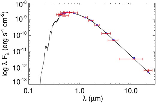
The spectral energy distribution of TOI-1789. The Red markers with the horizontal error bars denote the photometric measurements in each filter and their bandwidth, while the vertical error bars shows the measurement uncertainty. The Black curve is representing the best fit Kurucz stellar atmosphere model with highlighted blue circles as the model fluxes over each passband.
Priors along with Median values and 68 per cent confidence interval for TOI-1789 from EXOFASTv2. The |$\mathcal {N}$| and |$\mathcal {U}$| represents the Gaussian and the Uniform priors, respectively.
| Parameter | Units | Adopted Priors | Values | |
|---|---|---|---|---|
| Stellar Parameters: | ||||
| M*.... | Mass (M).... | – | |$1.507^{+0.059}_{-0.14}$| | |
| R*.... | Radius (R).... | – | |$2.168^{+0.036}_{-0.034}$| | |
| L*.... | Luminosity (L).... | – | |$5.45^{+0.15}_{-0.14}$| | |
| ρ*.... | Density (cgs).... | – | |$0.208^{+0.014}_{-0.020}$| | |
| log g.... | Surface gravity (cgs).... | – | |$3.943^{+0.023}_{-0.043}$| | |
| Teff.... | Effective temperature (K).... | |$\mathcal {N}$|(5894, 142) | 5991 ± 55 | |
| [Fe/H].... | Metallicity (dex).... | |$\mathcal {N}$|(0.38, 0.1) | |$0.373^{+0.071}_{-0.086}$| | |
| Age.... | Age (Gyr).... | – | |$2.73^{+1.3}_{-0.51}$| | |
| EEP.... | Equal evolutionary point .... | – | |$404^{+45}_{-14}$| | |
| AV.... | V-band extinction (mag).... | |$\mathcal {U}$|(0, 0.067) | |$0.030^{+0.025}_{-0.021}$| | |
| σSED.... | SED photometry error scaling .... | – | |$2.78^{+0.74}_{-0.52}$| | |
| vsin i.... | Projected rotational velocity (km s−1).... | – | 7.0 ± 0.5 | |
| ϖ.... | Parallax (mas).... | |$\mathcal {N}$|(4.4743, 0.0181) | 4.474 ± 0.018 | |
| d.... | Distance (pc).... | – | |$223.53^{+0.91}_{-0.90}$| | |
| Planetary Parameters: | b | |||
| P.... | Period (days).... | −- | 3.208664 ± 0.000015 | |
| RP.... | Radius (|$\, R_{\rm J}$|).... | – | |$1.44^{+0.24}_{-0.14}$| | |
| TC.... | Time of conjunction (|$\rm {BJD_{TDB}}$|).... | – | 2458873.65374 ± 0.00062 | |
| a.... | Semimajor axis (AU).... | – | |$0.04882^{+0.00063}_{-0.0016}$| | |
| i.... | Inclination (Degrees).... | – | |$78.41^{+0.36}_{-0.58}$| | |
| Teq.... | Equilibrium temperature (K).... | – | |$1927^{+27}_{-17}$| | |
| MP.... | Mass (|$\, M_{\rm J}$|).... | – | 0.70 ± 0.16 | |
| K.... | RV semi-amplitude (m/s).... | – | |$72^{+17}_{-16}$| | |
| logK.... | Log of RV semi-amplitude .... | – | |$1.861^{+0.090}_{-0.11}$| | |
| RP/R*.... | Radius of planet in stellar radii .... | – | |$0.0680^{+0.011}_{-0.0061}$| | |
| a/R*.... | Semi-major axis in stellar radii .... | – | |$4.83^{+0.11}_{-0.16}$| | |
| δ.... | Transit depth (fraction).... | – | |$0.00463^{+0.0016}_{-0.00080}$| | |
| Depth.... | Flux decrement at mid transit .... | – | |$0.00347^{+0.00020}_{-0.00018}$| | |
| T14.... | Total transit duration (days).... | – | 0.0959 ± 0.0018 | |
| b.... | Transit Impact parameter .... | – | |$0.972^{+0.017}_{-0.011}$| | |
| ρP.... | Density (cgs).... | – | |$0.28^{+0.14}_{-0.12}$| | |
| loggP.... | Surface gravity .... | – | |$2.91^{+0.14}_{-0.18}$| | |
| 〈F〉.... | Incident flux (109 erg s−1 cm−2).... | – | |$3.13^{+0.18}_{-0.11}$| | |
| MPsin i.... | Minimum mass (|$\, M_{\rm J}$|).... | – | |$0.68^{+0.16}_{-0.15}$| | |
| MP/M*.... | Mass ratio .... | – | 0.00045 ± 0.00010 | |
| Wavelength Parameters: | R | TESS | ||
| u1.... | Linear limb-darkening coeff .... | 0.356 ± 0.035 | |$0.263^{+0.046}_{-0.047}$| | |
| u2.... | Quadratic limb-darkening coeff .... | |$0.309^{+0.035}_{-0.034}$| | 0.284 ± 0.047 | |
| Telescope Parameters: | PARAS | TCES | ||
| γrel.... | Relative RV Offset (m/s).... | −93 ± 12 | |$122^{+14}_{-13}$| | |
| σJ.... | RV Jitter (m/s).... | |$26^{+14}_{-12}$| | |$51^{+14}_{-11}$| | |
| |$\sigma _J^2$|.... | RV Jitter Variance .... | |$730^{+960}_{-510}$| | |$2700^{+1700}_{-1000}$| | |
| Transit Parameters: | PRL ADR (R) | PRL TRI (R) | TESS (TESS) | |
| σ2.... | Added Variance .... | |$0.00000252^{+0.00000025}_{-0.00000023}$| | |$0.00000015^{+0.00000018}_{-0.00000016}$| | |$0.0000000064^{+0.0000000018}_{-0.0000000017}$| |
| F0.... | Baseline flux .... | 1.00006 ± 0.00010 | |$1.000509^{+0.000100}_{-0.000099}$| | 0.9999953 ± 0.0000061 |
The PDF of stellar mass and age (and their correlated parameters) show bimodality, which can be seen in Fig. A1. This type of bimodality has been observed in several recent studies (Grieves et al. 2021; Ikwut-Ukwa et al. 2020; Carmichael et al. 2020, 2021; Pepper et al. 2020) and it appears due to the degeneracy between the MIST isochrones in the region of Teff– log g* plane occupied by TOI-1789. The two peaks in the PDF are centred at a mass of 1.35 (age = 4.15 Gyr) and 1.51 M⊙ (age = 2.71 Gyr) with the probability of 30 and 70|${{\ \rm per\ cent}}$|, respectively. We finally adopted the solution provided by EXOFASTv2, which is centred at the most probable values for M*, age, and their correlated parameters and thus have larger uncertainties considering the bimodality. The adopted stellar parameters along with 1σ uncertainties are displayed in Table 4.
The final adopted values for the host star are log g* = |$3.943^{+0.023}_{-0.043}$|, |$\, M_*$| = |$1.507^{+0.059}_{-0.14}$| M⊙, |$\, R_*$| = |$2.168^{+0.036}_{-0.034}$| R⊙, at an age of |$2.73^{+1.3}_{-0.51}$| Gyr. The log g* determined here is slightly lower (∼ 1.3σ) than the one estimated with SME (Section 3.1.1). Stellar gravity is more accurately determined with SED, isochrones combined with the transit data which places a strong constraint on the stellar density of the star (Stevens et al. 2017). Therefore, we adopt the stellar parameters obtained from this global modelling to determine the orbital and planetary parameters.
3.3.2 Orbital parameters
The independent fit of one data set (either RV or transit) is useful in constraining mutually independent parameters obtained from either of these data sets. For e.g. b, i, Rp, and a are exclusively dependent on the transit data, while K and hence Mp depends on the RV data. However, the parameters like P, Tc, ω, and e depend on both the data sets and can be well constrained by fitting them simultaneously.
We use the photometry data from TESS and PRL (two data sets, Section 2.2), and RV data from PARAS and TCES for the simultaneous fitting. We provide the Gaussian priors on the stellar parameters derived in Section 3.3.1, along with the starting values for P and Tc given by the TESS QLP pipeline. We also include offsets and jitter terms for each data set of each instrument in RV and LC fitting. The transit model is generated using the Mandel & Agol (2002); re-sampling the transit model over 10 steps to account for the TESS long cadence (30 min) data (Kipping 2010). The photometric data were modeled with a quadratic limb-darkening (LD) law for TESS and Bessel-R (PRL transits) passbands. The u1 and u2 are derived by the interpolation of the Claret & Bloemen (2011), Claret (2017) LD models. We used 56 chains and 50 000 steps for MCMC global fitting, which allowed the fit to converge. First, we fit a circular orbit model keeping eccentricity to zero, and then an eccentric orbit model, by keeping the ecos ω* and esin ω* as free parameters to check for any significant eccentricity in the orbit. The eccentricity is found to be 0.1 ± 0.075. We calculated the Akaike Information Criterion (AIC, Akaike 1974) as well as Bayesian Information Criterion (BIC, Burnham & Anderson 2002) for both the models and find the ΔAIC between the models to be 6.0, moderately favouring the circular model over the eccentric model, while the ΔBIC to be 17.0, strongly supporting the circular orbit model. Thus, we adopted the circular orbit model and report the orbital and planetary parameters in Table 6. We find that TOI-1789 b has a mass of 0.70 ± 0.16 |$\, M_{\rm J}$| and a radius of |$1.44^{+0.24}_{-0.14}$| |$\, R_{\rm J}$|, which corresponds to the density of |$0.28^{+0.14}_{-0.12}$| g cm−3. The resulting best-fitting models from EXOFASTv2 for the transit LCs are plotted in Fig. 2, and for the RVs in Fig. 9. Fig. A1 shows the covariances for all the fitted parameters for the global joint fit. For TOI-1789, b + Rp/R* > 1 represents a grazing transit configuration. In such cases, the posterior probability densities contain a strong degeneracy between the transit impact parameter b (and its related parameters such as inclination, etc.) and the planetary radius Rp/R*. Due to this, the planetary radius can not be determined precisely. It can be seen for TOI-1789 in Fig. A1, there is degeneracy between Rp/R* and inclination cos i. Although we have used short cadence data along with TESS data and the transit is deeper (0.25|${{\ \rm per\ cent}}$|), the radius is not well constrained, having 9–16 |${{\ \rm per\ cent}}$| uncertainty.
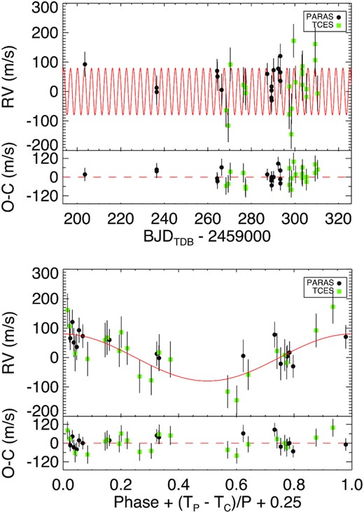
TOI-1789 RVs from PARAS (black dots), and TCES (green squares) are plotted here with respect to time in the upper panel, and with respect to orbital phase (∼ 3.21 d) in the lower panel, after subtracting the corresponding instrumental RV offsets γrel, listed in Table 6. The red line represents the best-fitting RV model for the planet from EXOFASTv2 (see Section 3.3.2). The bottom panel shows the residuals between the data and the best-fitting model.
4 DISCUSSION
TOI-1789, with its precise determination of host star and planet properties (with the precision of 22 and 9–16 |${{\ \rm per\ cent}}$| in planetary mass and radius, respectively), makes an important contribution to the study of gas giant planets around slightly evolved stars. In our discussion, we focus on the evolutionary status of the host star and the derived planet properties.
4.1 The evolved star
Semi-analytical disc models indicate that the frequency of giant planets must increase with the mass of the host star between 0.2–1.5 M⊙ (Ida & Lin 2005; Kennedy & Kenyon 2008). However, this trend is expected to decrease above 1.5 M⊙ due to a smaller growth rate, longer migration time-scale, and shorter lifetime of the protostellar disc (Reffert et al. 2015). Looking for planets around main sequence stars more massive than the sun can help shed some light on this aspect. These stars have few spectral lines for Doppler measurements and are often broadened by the rapid rotation of the star. This has been the reason for RV surveys to have traditionally targeted slow rotating FGK type stars. However, as rapidly rotating stars evolve off the main sequence they slow down considerably and become much cooler making it relatively easy to search for planets around them. This fact was exploited by dedicated planet searches around intermediate mass sub-giants leading to dozens of planet discoveries (Johnson et al. 2007, 2010a, 2011). An important result obtained from the survey of giant stars at the Lick observatory pointed out that the occurrence rate peaks at a stellar mass of |$1.9^{+0.1}_{-0.5}$| M⊙. However, many of the discovered planets around evolved stars were found at large orbital separations (Hatzes et al. 2003; Fischer et al. 2007; Robinson et al. 2007; Johnson et al. 2008). This is not a surprise as star–planet interaction is largely governed by tidal forces. When the stellar rotational period is longer than the planet orbital period, the star experiences spinning up, leading to orbital decay. Synchronization and circularization of orbit occurs in systems where the total angular momentum exceeds a critical value. When this total angular momentum is small enough, the orbit of the planet can continue to shrink and be engulfed by the host star. This phenomenon entirely depends on the dissipation time-scales for the star (Mazeh 2008, and references therein). The role of tidal forces becomes increasingly important in the context of host stars being in an evolved state. There is a higher chance of the planet being destroyed by the evolved star (Kunitomo et al. 2011; Schlaufman & Winn 2013). However, there is no obvious way to estimate these tidal dissipation forces. The circularization time-scale for such planets can be used to quantify tidal dissipation inside planets (Hansen 2010; Socrates et al. 2012). Most of the discovered hot Jupiters with periods less than 3 d are found to be on circular orbits. We calculate the circularization time-scales for the orbit of TOI-1789 b, which is τcir = 0.08 Gyr (for QP = 106, equation 3 of Adams & Laughlin 2006). This is less than the age of the star as calculated from our work (Section 3.3.1).
Fig. 10 shows all the transiting hot Jupiters taken from the Transiting ExoPlanet catalogue (TEPcat) database11 with uncertainties on the masses and radii < 25 per cent. We use a planet mass cut off between 0.25MJ < M < 13MJ and orbital period less than 10 d to stay consistent with the definition of hot Jupiter (Boss et al. 2005; Dawson & Johnson 2018). We plot log g* as an indicator of the evolutionary status of the star versus the separation of the host star (a) from its orbiting planet in AU. Stars are colour-coded according to their metallicity. Stars with high metallicity appear as yellow, whereas the ones with sub-solar metallicities are blue. The size of the individual points represent the planet’s mass. We mark the position of TOI-1789 with the arrow, and is labelled as red text in the figure. One notes that close-in transiting planets are more common around the main sequence stars (log g* ≥ 4.1). Another thing to notice is that most of the planet host stars have supersolar metallicity. This correlation of stellar metallicity with planet occurrence rate for main-sequence stars was reported early on by Gonzalez (1997), Santos, Israelian & Mayor (2004), Fischer & Valenti (2005). There were surveys like the Next 200 Stars (N2K) and ELODIE survey which were particularly designed to utilize this information discovering several Jovian exoplanets (Bouchy et al. 2005; Fischer et al. 2005; Moutou et al. 2006). The study of the planet–metallicity relation was extended to evolved stars thanks to the survey of giant stars carried out at the Lick Observatory (Frink et al. 2001). A strong planet–metallicity correlation with a power-law exponent of |$1.7^{+0.3}_{-0.4}$| was reported from this survey (Reffert et al. 2015). With a derived metallicity of |$0.373^{+0.071}_{-0.086}$| dex, TOI-1789 joins the many other metal-rich host stars.
The surface gravity (log g*) of host stars having the transiting hot Jupiters (0.25MJ < M < 13MJ and P<10 d) in their orbits are plotted as a function of orbital separation (a) in au. Data sets used in this diagram are taken from the TEPcat database12, and only planets with uncertainty on the masses and radii <25|${{\ \rm per\ cent}}$| are considered. Metallicity of the host star is colour-coded, with colours ranging from low metallicity (in blue) to high metallicity (in yellow). The size of individual dots represent the planet’s mass in Jupiter mass. The grey shaded region represents the boundary (a ≤ 0.05 au and log g* ≤ 4.1 dex) and the other seven exoplanets as described in Section 4.1 can be seen under this shaded region. The position of TOI-1789 marked with arrow and is labeled as red text in the figure.
Given any stellar type, there is a detection bias favouring close-in planets. We see from Fig. 10 that there are fewer planets situated to the proximity of their host stars for the case of evolved stars (log g < 4.1) as compared to the main-sequence stars. This dearth of close-in planets around sub-giants and giant stars was also noted by Bowler et al. (2010). The surface gravity of host star (log g*) shows a weak linear correlation with a as seen from this figure (Pearson correlation coefficient = –0.34, p = 8.2 × 10⁻¹²). This plot is representative of the fact that the proximity of the orbiting planets depends on the evolutionary status of the host star. TOI-1789 b is fairly close-in located at a distance of 0.048 au from its host star and seems to lie very close to this boundary. This boundary could be dictated by the fact that such close-in planets could be engulfed by its host star in the course of evolution on its sub-giant/giant phase. This fact is also supported by the masses of the planets seen close to this boundary limit. Most of these close-in planets have sub-Jovian to Jovian-like masses. Tidal forces are expected to be larger when the orbiting planet has a larger mass (Mazeh 2008). As of now, only eight planetary systems (including this work) around stars similar to or more evolved than TOI-1789 are known, which are orbiting closer to their host star (a ≤ 0.05 au). These are namely, [HATS-12: Rabus et al. (2016), HATS-26: Espinoza et al. (2016), HATS-40: Bento et al. (2018), WASP-71: Smith et al. (2013), WASP-78: Smalley et al. (2012), WASP-82: West et al. (2016) and WASP-165: Lendl et al. (2019)]. We mark this boundary (a ≤ 0.05 au and log g* ≤ 4.1 dex) with the shaded grey region in Fig. 10. At the age of ∼ 2.7 Gyr, TOI-1789 is a slightly evolved late F-type star with log g* of ∼ 3.9, a radius of ∼ 2.2R⊙ and a mass of ∼ 1.5 M⊙. The circular orbit for the planet seen here is evidence of the strong tidal interaction due to its host star. This makes TOI-1789 b a rare and important system in understanding the evolution of close-in planets around stars transiting off their main sequence.
4.2 The heated planet
Understanding the radius inflation of transiting hot giants is an important aspect of exoplanetary science. The determination of precise stellar ages is useful in this context. Finding inflated Jupiters during the end-of-main sequence phase is indicative of a deep heating mechanism. However, if hot Jupiters are found to be inflated during the post-main-sequence, then heating must be concentrated at deposition pressure ≥105 bars (Komacek et al. 2020). Considering the aspects of both stellar irradiation and the age of the system, Komacek et al. (2020) postulated that inflated Jupiters would be the most common around stars with masses 1.0 <M* <1.5 M⊙, which is also true for TOI-1789 which has a mass of |$1.507^{+0.059}_{-0.14}$| M⊙ and the radius of the planet of |$1.44^{+0.24}_{-0.14}$| RJ. Fig. 11 shows the data for the known transiting hot Jupiters from the TEPcat database,12 where we plot the planet radius against its equilibrium temperature. The size of the individual dots on this figure corresponds to the mass of the planet. We mark the position of TOI-1789 b as a red asterisk symbol. It has a fairly inflated radius relative to its mass. The equilibrium temperature for the planet (assuming no albedo and perfect redistribution) is estimated to be |$1927^{+27}_{-17}$| K. Several studies indicate that inflation in hot Jupiters would be due to the high incident fluxes received by them through their host stars (Guillot & Showman 2002; Tremblin et al. 2017; Sainsbury-Martinez et al. 2019). The total incident flux received by TOI-1789 b is |$3.13^{+0.18}_{-0.11} \times 10^9$| erg s−1 cm−2. This flux-limit is more than 15 times the threshold (2 × 10⁸ erg s−1 cm−2), as described in Demory & Seager (2011), below which there is no chance of finding inflated hot Jupiters.
The planetary radius-equilibrium temperature relation diagram for known transiting hot Jupiters (0.25MJ < M < 13MJ and p< 10 d. Data are taken from the TEPcat database12, only planets with uncertainty on the masses and radii <25|${{\ \rm per\ cent}}$| are considered. The size of individual dots correspond to the mass of the planet in terms of Jupiter. The position of TOI-1789 b is plotted as red asterisk symbol.
Inflated planets are considered good candidates to study their atmospheric properties via transits (Charbonneau et al. 2005; Winn 2008; Southworth 2009). TOI-1789 b has a very low bulk density of |$0.28^{+0.14}_{-0.12}$| g cm–3. Assuming a hydrogen-rich atmosphere and thereby a μ of 2.3, we calculate the scale height (H = KbTeq/μg) (Madhusudhan et al. 2014) of 852 km. The transmission spectroscopy metric (TSM) for this target as noted in TFOP observing notes is 210.8. Based on the formulation from Kempton et al. (2018) and our derived parameters from this work, we re-calculate the TSM as 139.4. This places TOI-1789 in the top two quartiles for the sub-Jovian planets suitable for high-priority atmospheric characterization as noted by Kempton et al. (2018). Despite this scale height and TSM, the expected amplitude of spectral features in transmission is only ∼ 0.016|${{\ \rm per\ cent}}$| (Kreidberg 2018) due to the large radius of the host star. Thus, TOI-1789 might not be the ideal target for ground-based transmission spectroscopy studies but can be a suitable candidate for future JWST12 or ARIEL studies (Tinetti et al. 2016).
Due to its unique position in the evolutionary state and a relatively bright magnitude, TOI-1789 is a good choice to study the Rossiter–McLaughlin (R-M) effect. Most hot Jupiters are aligned in their orbits with the spin angle of their host stars. However, some of these can also be misaligned (Albrecht et al. 2012). R-M effect (McLaughlin 1924; Rossiter 1924) can be used to study this projected stellar obliquity of planets. Based on the larger stellar radius and its relatively high v sin i, RM semiamplitude could be between 2.5 and 16 m s−1 for the projected spin-orbit angle (λ) between 0° and 90°, respectively (Ohta, Taruya & Suto 2005). Depending on the projected spin-orbit angle, this can be observed with any moderate-sized telescope (2.5–4-m aperture) with a precise RV instrument.
5 SUMMARY
We have presented the discovery and characterization of a transiting hot Jupiter, TOI-1789 b, from TESS photometry data, follow-up ground-based photometry data from PRL, along with precise RV data from PARAS and TCES spectrographs. Based on the global modelling of these photometry and RV data sets, the host star has a mass of |$1.507^{+0.059}_{-0.14}$| M⊙, radius of |$2.168^{+0.036}_{-0.034}$| R⊙, metallicity of |$0.373^{+0.071}_{-0.086}$| dex, effective temperature of 5991 ± 55 K, and surface gravity (log g*) of |$3.943^{+0.023}_{-0.043}$| that indicate it is a slightly evolved, metal-rich, and late F-type star. The planetary parameters for TOI-1789 b are as follows: |$\, M_{\rm P}$|: 0.70 ± 0.16 |$\, M_{\rm J}$|, |$\, R_{\rm P}$|: |$1.44^{+0.24}_{-0.14}$| |$\, R_{\rm J}$|, ρP: |$0.28^{+0.14}_{-0.12}$| g cm−3, and Teq: |$1927^{+27}_{-17}$| K. At a 4σ significance on the derived mass and radius for TOI-1789 b, we find the radius of TOI-1789 b to be inflated for its planetary mass. TOI-1789 b could have already been circularized as seen from our results. This is in agreement with the calculated circularization time-scale of 0.08 Gyr, which is less than the estimated age of the system. There are only 8 exoplanets (including TOI-1789 b) discovered as of now, which are hosted by either similar or more evolved stars than TOI-1789 and orbiting in very close-proximity to their host star (a ≤ 0.05 au). Despite the rarity of hot Jupiters across slightly evolved stars in close-in orbits, TOI-1789 b is completely ‘non-anomalous,’ satisfying most of the evolutionary models at place. The detection of similar types of exoplanets will help us to improve our understanding of the distribution, formation, and migration of hot Jupiters around evolving stars.
ACKNOWLEDGEMENTS
We acknowledge the PRL-DOS (Department of Space, Government of India) and the director of PRL for supporting the PARAS spectrograph funding for the exoplanet discovery project and the research grant for AK. PC acknowledges the generous support from Deutsche Forschungsgemeinschaft (DFG) of the grant HA3279/11-1. We are grateful for the generous support by Thüringer Ministerium für Wirtschaft, Wissenschaft und Digitale Gesellschaft. CMP and MF gratefully acknowledge the support of the Swedish National Space Agency (DNR 65/19-P). We acknowledge the help from Kapil Kumar, Vishal Shah, and all the Mount-Abu and TLS observatory staff for their assistance during the observations. We are grateful to the user support group of the Alfred Jensch telescope at Tautenburg, Germany. AC is grateful to Suvrath Mahadevan and Arpita Roy from Pennsylvania University, USA, for their tremendous efforts in developing the PARAS data pipeline in 2014. We thank Mathias Zechmeister and Jana Koehler for their help in the ongoing development of the viper pipeline. Some of the observations in the paper made use of the High-Resolution Imaging instrument ‘Alopeke obtained under Gemini LLP Proposal Number: GN/S-2021A-LP-105. ‘Alopeke was funded by the NASA Exoplanet Exploration Program and built at the NASA Ames Research Center by Steve B. Howell, Nic Scott, Elliott P. Horch, and Emmett Quigley. Alopeke was mounted on the Gemini North (and/or South) telescope of the international Gemini Observatory, a program of NSF’s OIR Lab, which is managed by the Association of Universities for Research in Astronomy (AURA) under a cooperative agreement with the National Science Foundation. On behalf of the Gemini partnership: the National Science Foundation (United States), National Research Council (Canada), Agencia Nacional de Investigación y Desarrollo (Chile), Ministerio de Ciencia, Tecnología e Innovación (Argentina), Ministério da Ciência, Tecnologia, Inovações e Comunicações (Brazil), and Korea Astronomy and Space Science Institute (Republic of Korea). This research has made use of the SIMBAD database (Wenger et al. 2000), operated at CDS, Strasbourg, France. This research has made use of the Exoplanet Follow-up Observation Program website, which is operated by the California Institute of Technology, under contract with the National Aeronautics and Space Administration under the Exoplanet Exploration Program. This paper includes data collected with the TESS mission, obtained from the MAST data archive at the Space Telescope Science Institute (STScI). Funding for the TESS mission is provided by the NASA Explorer Program. STScI is operated by the Association of Universities for Research in Astronomy, Inc., under NASA contract NAS 5-26555. This work has made use of the ASAS3, SuperWASP, Keck archives, and the Transiting ExoPlanet catalogue (TEPcat) database. The following software were used in research for this paper: AstroImageJ (Collins et al. 2017), PARAS|$\_$|PIPELINE (Chakraborty et al. 2014), EXOFASTv2 (Eastman et al. 2019), george kernel (Ambikasaran et al. 2015), juliet (Espinoza et al. 2019), Astropy (Astropy Collaboration et al. 2018), lightkurve (Lightkurve Collaboration et al. 2018), viper (Zechmeister et al. 2021), and PyAstronomy (Czesla et al. 2019).
DATA AVAILABILITY
The TESS photometry and the high-resolution speckle imaging data underlying this article are available at the Mikulski Archive for Space Telescopes (MAST) (https://mast.stsci.edu/) and the ExoFOP-TESS webpage (https://exofop.ipac.caltech.edu/tess/target.php?id = 172518755), respectively. The radial velocity measurements are provided in the Table 5. All other data underlying this article will be shared on reasonable request to the corresponding author.
Footnotes
https://www.astro.keele.ac.uk/jkt/tepcat/ Southworth (2011) as of June 9, 2021
REFERENCES
APPENDIX A: THE CORNER PLOT SHOWING THE COVARIANCES FOR ALL THE FITTED PARAMETERS FOR THE TOI-1789 GLOBAL-FIT
Corner plot of the fitted parameters involved in the global modelling of TOI-1789.
