


ABSTRACT
We present a comprehensive study of three large long-duration flares detected on an active M-dwarf binary EQ Peg using the Soft X-Ray Telescope of the AstroSat observatory. The peak X-ray luminosities of the flares in the 0.3–7-keV band are found to be within ∼5–10 × 1030|$\rm {erg}~\rm {s}^{-1}$|. The e-folding rise- and decay-times of the flares are derived to be in the range of 3.4–11 and 1.6–24 ks, respectively. Spectral analysis indicates the presence of three temperature corona with the first two plasma temperatures remain constant during all the flares and the post-flare observation at ∼3 and ∼9 MK. The flare temperature peaked at 26, 16, and 17 MK, which are 2, 1.3, and 1.4 times more than the minimum value, respectively. The peak emission measures are found to be 3.9–7.1 × 1053 cm−3, whereas the abundances peaked at 0.16–0.26 times the solar abundances. Using quasi-static loop modelling, we derive loop lengths for all the flares as 2.5 ± 0.5 × 10¹¹, 2.0 ± 0.5 × 10¹¹, and 2.5 ± 0.9 × 1011 cm, respectively. The density of the flaring plasma is estimated to be 4.2 ± 0.8 × 10¹⁰, 3.0 ± 0.7 × 10¹⁰, 2.2 ± 0.8 × 1010 cm−3 for flares F1, F2, and F3, respectively. Whereas the magnetic field for all three flares is estimated to be <100 G. The estimated energies of all three flares are ≳ 1034–1035erg, putting them in a category of superflare. All three superflares are also found to be the longest duration flares ever observed on EQ Peg.
1 INTRODUCTION
Flares on the Sun and stars are the most extreme evidence of magnetic activity in solar/stellar atmospheres. Our understanding of the flares is mostly developed on the basis of the Sun. Flares occur in close proximity to the active regions, which are the regions with localized magnetic fields. Magnetic loops from these active regions extend into the stellar corona. As the footpoints of these loops are jostled by the convective motions in the stars, they are twisted and distorted until magnetic reconnection occurs near the loop tops (Parker 1988; Benz & Güdel 2010). The reconnection process drives a rapid and transient release of magnetic energy in coronal layers, which is also associated with the electromagnetic radiation from radio waves to γ-rays. As a consequence, the charged particles are accelerated and gyrated downward along the magnetic field lines, producing synchrotron radio emission. These electron and proton beams then collide with the denser chromospheric materials, and hard X-rays (>20 keV) are emitted. Simultaneous heating of the plasma up to tens of MK evaporates the material from the chromospheric footpoints, which, in turn, increases the density of the newly formed coronal loops and emits at extreme UV and X-rays. Detailed and thorough investigations of these flaring events are useful to provide crucial information on the coronal structure.
On the Sun and magnetically active stars, flares are found to be associated with mass-loss due to coronal mass ejections (CMEs; Güdel 1997; Drake et al. 2000; Yashiro et al. 2006). In solar case, CMEs are observed to eject from 1013–1017 g of magnetized plasma into the interplanetary medium (e.g. Yashiro & Gopalswamy 2009; Vourlidas et al. 2010). Since most of the magnetically active cool stars can attain X-ray luminosities of about 1000 times more than that of the Sun, there is scope for vigorous CME activity, especially in the context of recent giant flare detections on solar-type stars (Maehara et al. 2012). Typically the solar flares emit the energy of 1029–1032 erg within the flare duration of several minutes to several hours. Stellar flares on solar-type stars with energies 1033–1038 erg are generally termed as ‘superflare’ (Schaefer, King & Deliyannis 2000; Shibayama et al. 2013). Although there are thousands of superflares, have been observed to date in optical and UV bands (Tu et al. 2020), but X-ray superflares are still very few (see Karmakar et al. 2017, and references therein). It is to be noted that most of the host stars of the X-ray superflares are either an M-dwarf or a binary or multiple systems with an M-dwarf component. Moreover, M-dwarfs show a higher level of magnetic activities than other solar-type stars (Suárez Mascareño, Rebolo & González Hernández 2016; Karmakar et al. 2019). This makes them very interesting objects to study.
M-dwarfs are the most populous low-mass stars with masses in the range of 0.6–0.075 |$\rm {M}_{\odot }$| (Baraffe & Chabrier 1996). All the M-dwarfs seem to show different levels of magnetic activities. Active M dwarfs of spectral types M0–M4 are known to be strong coronal X-ray sources with X-ray luminosities often close to the saturation limit of LX/Lbol ∼ 10−3.3 (Fleming et al. 1993; Pizzolato et al. 2003). These stars show frequent and strong flaring activities during which the X-ray luminosity increases by more than two orders of magnitude (e.g. Favata et al. 2000; Güdel et al. 2002; Schmitt et al. 2008). On the other hand, late M-dwarfs with spectral types M6–M9 are very faint X-ray sources during their quiescence, although they produce transient X-ray luminosity enhancements by orders of magnitude during flares (Rutledge et al. 2000; Schmitt & Liefke 2002; Stelzer et al. 2006). The magnetic field generation and subsequent activities in M-dwarfs are closely tied to stellar rotation and age (e.g. Mohanty & Basri 2003; Pizzolato et al. 2003; Kiraga & Stepien 2007). The faster a star rotates, the stronger its magnetic heating and surface activity. Since the angular momentum loss from magnetized winds slows rotation in M-dwarfs, magnetic activity also decreases with age.
The active M dwarf binary EQ Peg (BD + 19 5116, GJ 896) has a record of frequent and large flaring activities across the electromagnetic spectrum. With an age of 950 Myr (Parsamyan 1995), the visual binary system EQ Peg consists of an M3.5 primary (EQ Peg A) and an M4.5 secondary (EQ Peg B), separated by an angular separation of 5|${_{.}^{\prime\prime}}$|8 (Liefke et al. 2008). From Gaia DR2 observations, EQ Peg is found to be located at a distance of 6.260 ± 0.003 pc (Bailer-Jones et al. 2018). With V magnitudes of 10.35 and 12.4, both the primary and secondary components are well known optical flare stars (Lacy, Moffett & Evans 1976; Pettersen 1976). Microwave emission during quiescence was observed by Jackson, Kundu & White (1989), which they attributed to the brighter A component. Zboril & Byrne (1998) estimated a rotational velocity of 14 km s−1 for EQ Peg A, while Delfosse et al. (1998) analyzed the B component and derived the rotational velocity of 24.2 ± 1.4 km s−1; both v sin i values are rather high and thus consistent with a short rotation period system. Using SuperWASP transit survey data, Norton et al. (2007) derived a photometric period of 1.0664 d for the EQ Peg system. The EQ Peg system is a strong X-ray and extreme ultraviolet (EUV) source with a number of recorded flares. Pallavicini, Tagliaferri & Stella (1990) reported two flares observed with EXOSAT. The first one, with an atypically shaped light curve, was observed by Haisch et al. (1987) in the context of a simultaneous EXOSAT and International Ultraviolet Explorer (IUE) campaign. A second large-amplitude flare was observed by Pallavicini, Kundu & Jackson (1986). Another large flare was observed by Katsova, Livshits & Schmitt (2002) with ROSAT satellite with simultaneous optical photometry. A first approach to separate the A and B components in X-rays was undertaken with XMM–Newton (Robrade, Ness & Schmitt 2004). Although the two stars show considerable overlap owing to the instrumental point spread function, it was possible to attribute about three-quarters of the overall X-ray flux to the A component. A subsequent detailed spectral analysis without resolving the binary has been performed by (Robrade & Schmitt 2005). The first X-ray observation that allowed an unambiguous spectral separation of the two binary components was done with Chandra/HETG (Liefke et al. 2008). Morin et al. (2008) also found that the Zeeman Doppler Imaging map of EQ Peg A had a strong magnetic field spot of 0.8 kG, while EQ Peg B had a strong spot of 1.2 kG.
In this paper, we have investigated three superflares that occurred on the M-dwarf binary EQ Peg observed with the first Indian multi-wavelength space observatory AstroSat. All three flares are remarkable in their flare duration and the X-ray energies. We have organized the paper as follows. Observations and the data reduction procedure are discussed in Section 2. Analysis and results from X-ray timing and spectral analysis, along with the time-resolved spectroscopy, are presented in Section 3. Finally, in Section 4, we have discussed our results in light of the loop modelling, energetics, loop properties, CMEs, and magnetic field strengths and presented our conclusion.
2 OBSERVATIONS AND DATA REDUCTION
We have observed EQ Peg using Soft X-ray focusing Telescope (SXT; Singh et al. 2014, 2017), Large Area X-ray Proportional Counter (LAXPC; Antia et al. 2017), Cadmium Zinc Telluride Imager (CZTI; Bhalerao et al. 2017), and Ultra-Violet Imaging Telescope (UVIT; Tandon et al. 2017) onboard AstroSat observatory, during 2019 October 21–23 (PI. Karmakar; ID: A07_094T01_9000003248). We did not detect EQ Peg in hard X-ray during our observation, while the source was not observed with either near ultraviolet (NUV; 2000–3000 Å) or far ultra-violet (FUV; 1300-1800 Å) channels of UVIT. Since the visual (VIS; 3200–5500 Å) channel is only meant for aspect correction and not expected for science observation (Tandon et al. 2020), we have not used that in our analysis. In this paper, we have used the 0.3–7 keV AstroSat/SXT observations for further analysis. A detailed log of the observations of the source is given in Table 1. The level 1 data were processed using the AS1SXTLevel2-1.4b pipeline software to produce level 2 clean event files for each orbit of observation. We used the sxtevtmerger tool1 to merge the event files corresponding to each orbit to a single cleaned event file for further analysis. We extracted images, light curves, and spectra using the FTOOLS task xselect V2.4k, which has been provided as a part of the latest heasoft version 6.28. For our analysis, we used a circular region of a radius of 13 arcmin centred at the source position to extract source products, whereas multiple sources free circular regions of 2|$farcm$|6 radii have been chosen as background region. For spectral analysis, we used the spectral redistribution matrix file (sxt_pc_mat_g0to12.rmf), and ancillary response file (sxt_pc_excl00_v04_20190608.arf) provided by the SXT team.2 All the SXT spectra were binned to achieve a minimum of 10 count per bin. The spectral analysis was carried out in an energy range of 0.3–7 keV using the X-ray spectral fitting package (xspec; version 12.11.1 Arnaud 1996). The errors were estimated for a confidence interval of 68 per cent (Δχ2 = 1), equivalent to ± 1σ. In our analysis, the solar photospheric abundances (|$\rm {Z}_{\odot }$|) were adopted from Anders & Grevesse (1989), whereas we used the cross-sections obtained by Morrison & McCammon (1983) to model the equivalent hydrogen column density |$\rm {N_{H}}$|.
Observations log of EQ Peg with AstroSat: ObsID A07_094T01_9000003248.
| Orbit | Exp. Time | Start Time | End Time |
|---|---|---|---|
| No. | (ks) | (UTC) | (UTC) |
| 21972 | 1.086 | 2019-10-21 13:34:28 | 2019-10-21 14:47:58 |
| 21973 | 3.328 | 2019-10-21 14:07:57 | 2019-10-21 16:36:51 |
| 21974 | 3.582 | 2019-10-21 16:12:53 | 2019-10-21 18:18:31 |
| 21975 | 3.589 | 2019-10-21 17:47:35 | 2019-10-21 20:02:20 |
| 21976 | 3.114 | 2019-10-21 19:21:43 | 2019-10-21 21:45:29 |
| 21977 | 2.871 | 2019-10-21 21:09:35 | 2019-10-21 23:31:47 |
| 21978 | 2.707 | 2019-10-21 22:57:26 | 2019-10-22 01:18:18 |
| 21980 | 3.406 | 2019-10-22 00:51:47 | 2019-10-22 04:25:38 |
| 21981 | 1.595 | 2019-10-22 04:17:52 | 2019-10-22 06:11:53 |
| 21982 | 1.937 | 2019-10-22 05:48:01 | 2019-10-22 07:49:32 |
| 21984 | 2.184 | 2019-10-22 07:42:03 | 2019-10-22 09:58:17 |
| 21985 | 2.814 | 2019-10-22 09:08:04 | 2019-10-22 11:43:10 |
| 21986 | 2.524 | 2019-10-22 11:03:25 | 2019-10-22 13:27:29 |
| 21987 | 2.745 | 2019-10-22 13:14:53 | 2019-10-22 15:10:57 |
| 21988 | 3.404 | 2019-10-22 14:52:27 | 2019-10-22 16:59:24 |
| 21989 | 3.630 | 2019-10-22 16:28:49 | 2019-10-22 18:41:26 |
| 21990 | 3.416 | 2019-10-22 18:04:30 | 2019-10-22 20:23:13 |
| 21991 | 3.000 | 2019-10-22 19:56:00 | 2019-10-22 22:07:52 |
| 21992 | 3.000 | 2019-10-22 21:30:11 | 2019-10-22 23:55:50 |
| 21995 | 5.289 | 2019-10-22 23:22:36 | 2019-10-23 04:55:43 |
| 21996 | 0.404 | 2019-10-23 04:47:45 | 2019-10-23 05:50:52 |
3 ANALYSIS AND RESULTS
3.1 X-ray light curves
The background-subtracted 0.3–7 keV X-ray light is shown in the top panel of Fig. 1. The AstroSat/SXT observation of EQ Peg began at HJD = 2458778.06559 d (= T0). The light curve shows a large variation in SXT count rates from 0.4 to 1.6 count s−1 during the observation of ∼140 ks stare time. From the beginning of the observation until T0 + 20 ks, the light curve shows a constant count rate of ∼0.5 count s−1, which we term as the ‘pre-flare’ epoch. Whereas, a minimum count rate of ∼0.4 count s−1 has been observed during the observation from T0+120 ks to T0 + 140 ks, which we term as the ‘post-flare’ epoch.
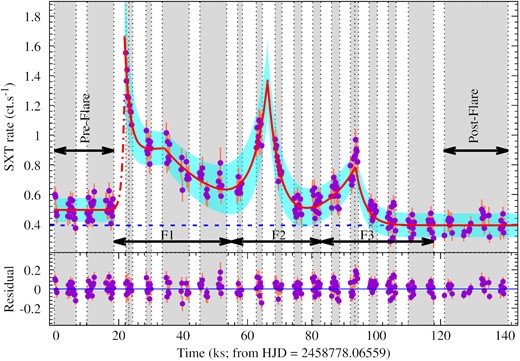
In the top panel, the background-subtracted AstroSat/SXT light curve of EQ Peg is shown in 0.3–7 keV energy band. The temporal binning of the light curve is 200 s. The solid red line shows the superimposed best-fitting model to the light curve. While the cyan shaded region shows the 1σ variations from the best-fitting model. The grey shaded regions separated by the vertical dotted lines show the different time intervals for which time-resolved spectroscopy is performed. The approximate duration of the flares (F1, F2, and F3), the ‘Pre-flare’, and the ‘Post-Flare’ segments have been marked with black arrows. The red dot-dashed line is an extrapolated exponential curve that indicates the rise phase of flare F1. In the bottom panel, the (data model) residual have been plotted. The evenly distributed residuals along the horizontal line corresponding to zero residual indicate that the model curve does not seem to show any systematic deviation from the data.


Spectral fitting to the AstroSat/SXT data have been shown for the time intervals as given in Fig. 1 and Table 2. In each of the figures (‘a’ to ‘s’), the upper panel shows the data with red triangles. The best-fitting 3-T apec model is shown with a solid blue line. The black dotted line, purple dot–dashed line, and orange dashed lines shows the unfolded 1-T, 2-T, and 3-T temperature component to the model, respectively. The bottom panel shows the residual in the unit of Δχ2. The top right-hand corner of the upper panel in each plot shows the segment number (i.e. P01–P19; as mentioned in Table 2). Here, flare F1, F2, and F3 corresponds to the segments P03–P07, P08–P12, and P13–P18, respectively. Whereas the segments P01–P02 and P19 indicate the ‘Pre-Flare’ and the ‘Post-Flare’ Spectra, respectively.
In this paper, in order to identify the flares, we have considered the positive count rate excursions greater than three times the standard deviation (σ) of the post-flare light curve. It is to be noted that, Fig. 1 shows an optimum light curve with a time binning of 0.2 ks, whereas median uncertainty in SXT count rate is ∼0.05 count s−1. Therefore, using the AstroSat/SXT observation the best precision in estimating τr and τd we can get is ∼3 min. On the other hand, since, to identify a flare, we need at least three consecutive points more than 3σ level, we cannot identify any flare which lasts for ≲10 min. Moreover, the timing characteristics of the AstroSat/SXT observations shows ∼45-min alternation between observation and data gap. This makes it more difficult to discriminate between long coherent flare profiles and a superposition of multiple shorter, smaller flares. From the AstroSat/SXT observation, we have identified three events (F1, F2, and F3) that can be significantly considered as flares. The identified flares have been shown with the black arrows in the top panel of Fig. 1.
Flares F1 started ∼T0+20 ks and extended until T0 + 58 ks, after reaching a peak count rate of ∼1.6 count s−1. The rise phase of flare F1 could not be observed due to the data gap. In Fig. 1, we have shown this by an extrapolated exponential curve with a red dot-dashed line. During the decay phase, instead of a simple exponential decay, it seems to have a plateau phase around 34 ks. If we fit a function containing a simple exponential decay (for the flare F1) and an exponential rise (for flare F2) in the time interval T0+20 to T0 + 65 ks, we find a systematic deviation around 34 ks, which results in the reduced χ2 value of 1.4 for 58 degrees of freedom (DOF). However, instead of a simple exponential decay, if we fit two exponential decay where the second one peaks around 34 ks, we get a better fit with a reduced χ2 value of 0.9 for 56 DOF as shown in the top panel of Fig. 1. This suggests that the decay of the flare F1 is best explained with a double-decay exponential. Either this might be due to a smaller flare superimposed to the flare F1, or the flare F1 is itself a double-decay flare. In order to verify if the plateau is likely to be a separate flare or not, we have detrended the data using the same function, but this time best-fitting was obtained excluding the plateau time interval T0+25 to T0 + 42 ks. We find that the AstroSat/SXT counts during the plateau time interval varies within a 1σ uncertainty level. Therefore, we can not significantly identify this as a separate flare. Therefore, for further analysis, we assume this plateau is a part of flare F1; rather, flare F1 is considered as a double-decay flare. The e-folding decay times for flare F1 are estimated to be 1.6 ± 0.4 and 24 ± 5 ks. This kind of double decay flare has been observed on plenty of low mass stars, such as AU Mic (Cully et al. 1993), UV Cet (Bopp & Moffett 1973), AD Leo (Gershberg & Chugainov 1967).
The flare F2 is found to start right after the flare F1 and ends around T0 + 84 ks after reaching a peak of >1.1 count s−1. From manual inspection, flare F2 is more likely peaked during the data gap near 68 ks. The flare F3 started just after the flare F2 and lasts until ∼T0 + 120 ks while it reaches up to a peak count rate of ∼1 count s−1. Both the flares F2 and F3 seems to show an exponential increase and exponential decay. From T0+68 to T0 + 93 ks, an exponential decay for flare F2 was fitted along with an exponential rise for flare F3 with best-fitting reduced χ2 value of 1.14 for 53 DOF. The fourth piece was fitted from T0+93 to T0 + 120 ks as an exponential decay for flare F3 with a best-fitting reduced χ2 value of 1.32 at 44 DOF. The e-folding rise times for flare F2 and F3 are estimated to be 3.4 ± 0.8 and 11 ± 2 ks, whereas the respective decay times are estimated to be 3.0 ± 0.6 and 3.1 ± 0.4 ks. This indicates that the rise and decay times in flares F2 are comparable in the soft X-ray band. However, flare F3 shows a comparatively slower rise than its decay.
3.2 Spectral analysis
In this section, we provide a detailed description of the X-ray spectral analysis of EQ Peg using AstroSat/SXT data. Since the spectral parameters evolve with time, to trace the changes in the source during the observation, we performed time-resolved spectroscopy. Considering the data-gap in the SXT light curve, in order to have approximately equal total counts in all the segments, we have divided the SXT light curves into nineteen segments (P01–P19), which includes five (P03–P07), five (P08–P12), and six (P13–P18) segments for the flares F1, F2, and F3, respectively, whereas two segments (P01 and P02) and one (P19) segment are for ‘Pre-Flare’ and ‘Post-Flare’. All these segments are shown with grey shaded regions, separated by vertical dotted lines in Fig. 1. Spectrum for each segment was extracted for further analysis.
3.2.1 Post-flare spectra
During the ∼140 ks of AstroSat observation of EQ Peg, no distinct quiescent state was observed. For preliminary analysis, therefore, as a starting point, we chose a segment with the lowest mean count rate as the ‘proxy’ of the quiescent phase. Although the segments P13 and P14 have similar lowest mean count rates, we chose ‘P14’ as the ‘Post-Flare’ region as the data in this segment might not have been contaminated due to the flare F3. The coronal parameters of the ‘Post-Flare’ phase were derived by fitting the spectrum with single (1-T), two (2-T), and three (3-T) temperatures Astrophysical Plasma Emission Code (apec; see Smith et al. 2001) as implemented for collisionally ionized plasma. The global abundances (Z) and interstellar H i column density (|$\rm {N_{H}}$|) were left as free parameters. None of the plasma models (1-T, 2-T, or 3-T) with solar abundances (|$\rm {Z}_{\odot }$|) was formally acceptable due to the large values of χ2. Although the 2-T model with sub-solar abundances was found to have a significantly better fit than that of the 1-T plasma model, the fitting is still unacceptable for the ‘Post-Flare’ spectrum as the value of reduced χ2 was 2.82 for 45 DOF. A 3-T plasma model improved the fitting significantly for the Post-Flare segment. The corresponding best-fitted spectra along with all the individual temperature components and the residuals are shown in Fig. 2(s). The best-fitting temperatures are derived to be 0.25 ± 0.02, 0.79 ± 0.04, and >1.09 keV for the Post-Flare segment. The corresponding global abundances were derived to be 0.37 ± 0.03, 0.41 ± 0.04, and >0.03 |$\rm {Z}_{\odot }$|. The unabsorbed X-ray Luminosity (LX) were calculated in 0.3–7 keV range using the CFLUX model for a distance of 6.260 ± 0.003 pc (Bailer-Jones et al. 2018). The LX is derived to be 2.7 × 1030 erg s−1, which is ∼17 times more luminous than the equivalent quiescent X-ray luminosity of EQ Peg, estimated from the Chandra/HETG observations (Liefke et al. 2008). This result indicates that the ‘Post-Flare’ is not the actual quiescent state of EQ Peg. In order to compute the equivalent quiescent luminosity, we have converted the flux from 2–25-Å Chandra/HETG band to 0.3–7 keV energy band using webpimms.3 For this conversion, we have considered a 3-T apec model of EQ Peg with the same parameters as derived in this section.
3.2.2 Flare spectra
As mentioned in Section 3.1, there are three flaring events detected during the SXT observation of EQ Peg. Spectra corresponding to all the segments during the flaring events were extracted and fitted with 1-T, 2-T, and 3-T plasma models. Among these three models, the 3-T plasma model was found to be acceptable for fitting the spectra of all the segments of flares F1, F2, and F3. In the beginning, the fitting was carried out by keeping all parameters such as three temperatures, normalizations, |$\rm {N_{H}}$|, and abundances free. While fitting, though |$\rm {N_{H}}$| was a free parameter, its value was found to be constant (within 1σ uncertainty level). Considering this, we fixed |$\rm {N_{H}}$| to its average value of 2.32 × 10²⁰ atoms cm−2. This average derived value of |$\rm {N_{H}}$| is marginally less than that estimated in a cone of 0.1 degrees in the direction of EQ Peg using the latest H i Pi survey (3.95 × 10²⁰ atoms cm−1; HI4PI Collaboration et al. 2016). Since the distance of EQ Peg is minimal compared to the thin disk scale height (∼300 pc; Gilmore & Reid 1983), it is unlikely that the large estimated value of the |$\rm {N_{H}}$| to be contributed from the interstellar medium between the Sun and EQ Peg. Instead, it is more likely that the estimated column density is due to the locally originated gas from EQ Peg. The first two temperatures, corresponding EMs, and corresponding abundances were found to be constant within the 1σ uncertainty level. The average values of the first two temperatures over all the segments are 0.24 ± 0.04 and 0.81 ± 0.06 keV, whereas the corresponding EMs are derived to be 6.98 ± 0.07 × 1052 and 6.04 ± 0.08 × 1052 cm−3, respectively. The abundances corresponding to the first two temperatures are also found to be equal ∼0.4 within 1σ uncertainty. These two temperatures, EMs, and abundances are found to be similar to that of the first two temperatures of the Post-Flare phase. Therefore, for the further spectral fitting of the flare-segments, we fixed the first two temperatures, corresponding EMs, and abundances at the average values. Only the third temperature (kT3), corresponding EM (EM3), and abundance (Z3) are allowed to vary while fitting the flaring segments and identified as flare components. The best-fitted spectra for all the segments along with the individual temperature components and the residuals are shown in Fig. 2. The time evolution of derived spectral parameters during the flares F1, F2, and F3 are shown in Fig. 3 using blue, orange, and cyan shaded regions, respectively. The other segments (i.e the Pre-Flare and Post-Flare segments) are shown with the grey shaded region. The derived spectral parameters from fitting the spectra from all the segments with a 3-T plasma model are given in Table 2.
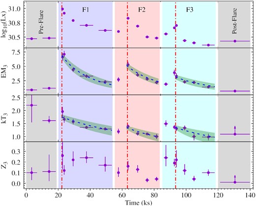
Evolution of spectral parameters of EQ Peg. From the top to bottom panels, the logarithmic values of X-ray luminosities as derived in 0.3–7-keV band, the emission measure (EM3) associated to flaring plasma, corresponding plasma temperature (kT3), and corresponding global abundance (Z3) have been shown. The blue, orange, and cyan shaded regions indicate the duration of flares F1, F2, and F3. The ‘Pre-Flare’ and ‘Post-Flare’ segments have been shown with the grey shaded region. The Horizontal bars give the time range over which spectra were extracted, and the vertical bars show a 68 per cent confidence interval of the parameters. The blue dashed line shows the best-fitting of equations (3) and (4) to the EM3 and kT3, respectively during the decay phase of each flare. The green shaded region shows the 1σ uncertainty in the fitting. The red dot–dashed vertical lines show the flare peak time t0 for each flare as mentioned in equations (3) and (4), and described in Section 4.1. The best-fitting quasi-static decay times estimated from each flare have been given in Table 3.
Best-fitting spectral parameters of EQ Peg obtained from the time-resolved spectroscopy of AstroSat/SXT observation.
| Flares | Segments | Timerange | kT3 | EM3 | Z3 | log10(Lx) | χ2 (DOF) |
|---|---|---|---|---|---|---|---|
| (ks) | (keV) | (1053 cm−3) | (|$\rm {Z}_{\odot }$|) | (cgs unit) | |||
| Pre-Flare | P01 | T0+0 – T0 + 6.79 | |$2.20_{-0.66}^{+0.87}$| | |$0.9_{-0.1}^{+0.1}$| | |$0.10_{-0.07}^{+0.05}$| | |$30.47_{-0.01}^{+0.01}$| | 1.046 (87) |
| P02 | T0+10.14 – T0 + 18.48 | |$1.61_{-0.10}^{+0.18}$| | |$1.2_{-0.2}^{+0.2}$| | |$0.11_{-0.09}^{+0.16}$| | |$30.48_{-0.01}^{+0.01}$| | 1.119 (119) | |
| F1 | P03 | T0+22.21 – T0 + 23.16 | |$1.96_{-0.19}^{+0.18}$| | |$6.6_{-0.6}^{+0.7}$| | |$0.26_{-0.13}^{+0.14}$| | |$30.99_{-0.01}^{+0.01}$| | 1.048 (87) |
| P04 | T0+23.16 – T0 + 24.33 | |$1.66_{-0.13}^{+0.13}$| | |$7.1_{-0.5}^{+0.6}$| | |$0.12_{-0.04}^{+0.05}$| | |$30.92_{-0.01}^{+0.01}$| | 0.945 (90) | |
| P05 | T0+28.48 – T0 + 30.18 | |$1.57_{-0.10}^{+0.11}$| | |$4.4_{-0.4}^{+0.4}$| | |$0.22_{-0.06}^{+0.08}$| | |$30.79_{-0.01}^{+0.01}$| | 1.028 (95) | |
| P06 | T0+33.52 – T0 + 41.87 | |$1.35_{-0.05}^{+0.06}$| | |$3.3_{-0.3}^{+0.3}$| | |$0.24_{-0.05}^{+0.06}$| | |$30.70_{-0.01}^{+0.01}$| | 1.094 (115) | |
| P07 | T0+45.21 – T0 + 53.56 | |$1.29_{-0.05}^{+0.06}$| | |$2.3_{-0.3}^{+0.3}$| | |$0.17_{-0.06}^{+0.08}$| | |$30.62_{-0.01}^{+0.01}$| | 1.054 (94) | |
| F2 | P08 | T0+56.90 – T0 + 58.46 | |$1.19_{-0.09}^{+0.11}$| | |$2.7_{-0.4}^{+0.4}$| | |$0.10_{-0.04}^{+0.05}$| | |$30.60_{-0.02}^{+0.02}$| | 1.043 (59) |
| P09 | T0+62.75 – T0 + 64.61 | |$1.39_{-0.08}^{+0.07}$| | |$5.3_{-0.4}^{+0.5}$| | |$0.16_{-0.04}^{+0.05}$| | |$30.83_{-0.01}^{+0.01}$| | 1.174 (110) | |
| P10 | T0+68.59 – T0 + 70.76 | |$1.11_{-0.07}^{+0.05}$| | |$3.5_{-0.3}^{+0.4}$| | |$0.13_{-0.03}^{+0.04}$| | |$30.69_{-0.01}^{+0.01}$| | 1.310 (92) | |
| P11 | T0+74.44 – T0 + 76.88 | |$1.10_{-0.05}^{+0.05}$| | |$2.8_{-0.3}^{+0.3}$| | |$0.03_{-0.02}^{+0.02}$| | |$30.50_{-0.02}^{+0.01}$| | 1.151 (68) | |
| P12 | T0+80.29 – T0 + 82.79 | |$1.00_{-0.10}^{+0.10}$| | |$2.2_{-0.3}^{+0.3}$| | |$0.04_{-0.02}^{+0.02}$| | |$30.48_{-0.02}^{+0.01}$| | 1.347 (69) | |
| F3 | P13 | T0+86.13 – T0 + 88.64 | |$1.49_{-0.11}^{+0.13}$| | |$1.9_{-0.3}^{+0.3}$| | |$0.24_{-0.08}^{+0.12}$| | |$30.55_{-0.01}^{+0.01}$| | 1.056 (83) |
| P14 | T0+91.98 – T0 + 93.35 | |$1.36_{-0.08}^{+0.08}$| | |$3.9_{-0.5}^{+0.5}$| | |$0.19_{-0.03}^{+0.04}$| | |$30.66_{-0.02}^{+0.02}$| | 0.992 (60) | |
| P15 | T0+93.35 – T0 + 94.48 | |$1.30_{-0.09}^{+0.09}$| | |$3.3_{-0.5}^{+0.5}$| | |$0.22_{-0.07}^{+0.09}$| | |$30.70_{-0.02}^{+0.02}$| | 1.248 (57) | |
| P16 | T0+97.82 – T0 + 100.33 | |$1.33_{-0.09}^{+0.09}$| | |$2.3_{-0.3}^{+0.3}$| | |$0.12_{-0.04}^{+0.06}$| | |$30.44_{-0.02}^{+0.02}$| | 1.042 (68) | |
| P17 | T0+103.72 – T0 + 106.17 | |$1.00_{-0.15}^{+0.15}$| | |$2.2_{-0.3}^{+0.3}$| | |$0.04_{-0.02}^{+0.03}$| | |$30.40_{-0.02}^{+0.02}$| | 1.072 (59) | |
| P18 | T0+109.99 – T0 + 117.86 | |$0.98_{-0.13}^{+0.13}$| | |$1.4_{-0.2}^{+0.2}$| | |$0.10_{-0.03}^{+0.03}$| | |$30.36_{-0.02}^{+0.02}$| | 1.412 (71) | |
| Post-flare | P19 | T0+121.20 – T0 + 139.90 | >1.09 | |$0.7_{-0.1}^{+0.1}$| | >0.03 | |$30.43_{-0.01}^{+0.01}$| | 1.208 (92) |
The kT3, EM3, Z3, and LX were found to vary during the flares. The peak values of abundances for flares F1, F2, and F3 were derived to be ∼0.26, ∼0.16, and ∼0.24 |$\rm {Z}_{\odot }$|, which were 9, 5, and 8 times more than that of the post-flaring region. The derived peak flare temperatures for F1, F2, and F3 are 2, 1.4, and 1.5 times more than the lowest observed third thermal component. The EM3 followed the flare light curve and peaked at a value of 7.1 × 1053, 5.3 × 1053, and 3.9 × 1053 cm−3 for the flares F1, F2, and F3, which are approximately 10, 8, and 6 times than that of the Post-Flare region, respectively. The peak values of log10(|$\rm {L}_{X}$|) in 0.3–7-keV energy band during flares F1, F2, and F3 are derived to be 30.99 ± 0.01, 30.83 ± 0.01, and 30.70 ± 0.02 (|$\rm {L}_{X}$| is in the unit of erg s−1). This shows that the flares F1, F2, and F3 are approximately 4, 3, and 2 times more luminous than that of the Post-Flare regions.
4 DISCUSSION AND CONCLUSIONS
In this section, we have presented the loop modelling, energetics, coronal properties, and mass-loss due to CMEs associated with the X-ray flares as observed on EQ Peg. We have also discussed our results in the light of present understanding.
4.1 Loop modelling
In order to estimated the quasi-static cooling time-scales, we have fitted equation (3) to the EM3 data and equation (4) to the kT3 data that were derived from the spectral fitting to the AstroSat/SXT data. The decay phase of the flares F1, F2, and F3 contain five (P03–P07), four (P09–P12), and four (P15–P18) data points, respectively. We have used the orthogonal distance regression technique to get the best fit considering uncertainties in both x–y directions. As a result, we estimate τqs, EM values for flares F1, F2, and F3 to be 22 ± 4, 22 ± 5, and 28 ± 10 ks with the best-fitting reduced χ2 (DOF) values of 0.7 (4), 0.8 (3), and 0.7 (3), respectively. Whereas the τqs, kT is estimated to be 25 ± 7, 18 ± 6, and 21 ± 11 ks with the best-fitting reduced χ2 (DOF) values of 0.6 (4), 0.7 (3), and 0.6 (3). In equations (3) and (4), two time-scales (τqs, EM and τqs, kT) are expected to be same when the flare cools quasi-statically. For all three flares F1, F2, and F3, we confirm that both the time scales are indeed same (within the errors) i.e. τqs, EM ≈ τqs, kT. Therefore, in the following analysis, we use τqs, EM as the cooling time-scale (= τqs) for all three flares, since it is better constrained than τqs, kT. The evaluated values of τqs for the flares F1, F2, and F3 are 22 ± 4, 22 ± 5, 28 ± 10 ks, respectively.
Loop Parameters derived for flares F1, F2, and F3 of EQ Peg.
| Sl. | Parameters | Flare F1 | Flare F2 | Flare F3 |
|---|---|---|---|---|
| 1 | τr (ks) | – | 3.4 ± 0.8 | 11 ± 2 |
| 2 | τd (ks) | 1.6 ± 0.4, 24 ± 5 | 3.0 ± 0.6 | 3.1 ± 0.4 |
| 3 | τqs, EM (ks) | 22 ± 4 | 22 ± 5 | 28 ± 10 |
| 4 | τqs, kT (ks) | 25 ± 7 | 18 ± 6 | 21 ± 11 |
| 5 | EM(t0) (1053 cm−3) | 6.9 ± 0.4 | 5.2 ± 0.5 | 3.3 ± 0.5 |
| 6 | kT(t0) (keV) | 1.75 ± 0.09 | 1.34 ± 0.08 | 1.30 ± 0.09 |
| 7 | log10(LX, max) (in cgs) | 30.99 ± 0.01 | 30.83 ± 0.01 | 30.70 ± 0.02 |
| 8 | L (1011 cm) | 2.5 ± 0.5 | 2.0 ± 0.5 | 2.5 ± 0.9 |
| 9 | a | 0.24 ± 0.04 | 0.37 ± 0.06 | 0.28 ± 0.07 |
| 10 | ne (1010 cm−3) | 4.2 ± 0.8 | 3.0 ± 0.7 | 2.2 ± 0.8 |
| 11 | p (102 dyn cm−2) | 2.4 ± 0.5 | 1.3 ± 0.3 | 0.9 ± 0.4 |
| 12 | V (1032 cm3) | 4 ± 2 | 6 ± 3 | 7 ± 5 |
| 13 | B (G) | 69–85 | 48–64 | 39–57 |
| 14 | HRV (10−2 erg s−1 cm−3) | 1.9 ± 0.7 | 1.1 ± 0.5 | 0.6 ± 0.5 |
| 15 | HR (1030 erg s−1) | 7.2 ± 0.5 | 6.5 ± 0.7 | 4.2 ± 0.7 |
| 16 | EX (1034 erg) | ∼12.7 | ∼5.7 | ∼2.4 |
| 17 | EH (1034 erg) | ≳15.2 | ∼4.2 | ≳1.3 |
| 18 | MCME (1018 g) | ∼9.3 | ∼5.8 | ∼3.5 |
| 19 | vesc (km s−1) | ∼5500 | ∼4600 | ∼3900 |
| 20 | EKE, CME (1035 erg) | ∼14 | ∼2 | ∼3 |
| 21 | Btot (G) | 106–146 | 58–82 | 59–77 |
Notes. 1, 2 – e-folding rise- and decay-time as derived from the light curve; 3, 4 – quasi-static decay times as derived by fitting equations (3) and (4) (see Section 4.1); 5 – Emission Measure related to flaring plasma at the flare peak; 6 – Temperature related to flaring plasma at the flare peak; 7 – X-ray Luminosity at the flare peak, estimated in 0.3–7 keV energy band; 8 – length of the flaring loops; 9 – loop aspect ratio i.e. diameter to length ratio of the loop; 10, 11 – Estimated maximum electron density and loop pressure at flare peak; 12 – loop volume of the flaring region; 13– Minimum magnetic field. 14 – Heating rate per unit volume; 15 – Total Heating rate; 16 – X-ray energy estimated using trapezoidal integration of the derived X-ray luminosity; 17 – Estimated energy during flare due to heating of the stellar corona; 18 – Ejected coronal mass during the flaring events; 19 – Outward escape velocity of ejected coronal mass; 20 – Kinetic energy of the ejected coronal mass; 21 – Total magnetic field required to produce the flare (see the text for a detailed description).
4.2 Energetics
A detailed assessment of the energy balance of the flares in the present case is not possible due to the lack of multiwavelength coverage and velocity information, which could help to assess the plasma kinetic energy. Using simple trapezoidal integration of the instantaneous X-ray luminosity, we estimated the total energy radiated in X-rays (EX) during flares F1, F2, and F3 are ∼12.7 × 1034, ∼5.7 × 1034, and ∼2.4 × 1034 erg. Over 38, 26, and 36 ks duration, the energy released in X-ray are equivalent to ∼13, ∼6, and ∼3 s of the bolometric energy output of the star (considering total bolometric energy of the primary and secondary components). With the assumption that the flaring loop is in the steady-state, using the scaling law of Rosner, Tucker & Vaiana (1978), we can estimate the heating rate per unit volume (|$HR_{V} = \frac{{\rm d} H}{{\rm d} V {\rm d} t} \simeq 10^5 ~ p^{7/6} ~ L^{-5/6}$|) at the peak of the flare as 1.9 ± 0.7, 1.1 ± 0.5, 0.6 ± 0.5 |$\rm erg ~ cm^{-3} ~ s^{-1}$| for flares F1, F2, and F3, respectively. The total heating rate (|$HR = \frac{{\rm d} H}{{\rm d}t} \simeq \frac{{\rm d} H}{{\rm d} V {\rm d} t} \times V$|) at the peak of the flare, was derived to be 7.2 ± 0.5 × 1030 for F1, 6.5 ± 0.7 × 1030 for F2, and 4.2 ± 0.7 × 1030|$\rm {erg}~\rm {s}^{-1}$| for F3, which are 74 per cent, 96 per cent, and 84 per cent of the flare maximum luminosity, respectively. This result suggests that X-ray radiation is one of the major energy loss terms during the flare. If we assume that the heating rate is constant for the initial rise phase and then decays exponentially, with an e-folding decay time similar to that of the light curve, then the total energy radiated during the flare is given by |$E_{\rm H} \sim \frac{d H}{{\rm d}t} \times (\tau _r + \tau _{\rm d})$|. The estimated values of total energy radiated during the flare are found to be ≳ 15.2 × 1034, ∼4.2 × 1034, ≳1.3 × 1034 erg. These values are of the same order as the estimated total energy radiated in the X-ray. All three flares are found to emit a large amount of flare energies (> 1033 erg), and hence can be classified as ‘superflares’.
4.3 Coronal properties
The X-ray luminosity during flares F1, F2, and F3 reaches up to ∼9.8 × 1030, ∼6.8 × 1030, and ∼5.0 × 1030|$\rm {erg}~\rm {s}^{-1}$|, respectively. Among the previously reported flares on EQ Peg, the largest flare was observed with the ROSAT HRI instrument (Katsova et al. 2002). The ROSAT flare had a peak |$\rm {L}_{X}$| of 1.36 × 1030|$\rm {erg}~\rm {s}^{-1}$| in 0.1–2.4 keV energy range. To compute an equivalent luminosity in the 0.3–7 keV range, we considered 3-T apec model as derived in this paper. Using webpimms,4 the estimated values of the peak |$\rm {L}_{X}$| of the largest flare with ROSAT was 1.56 × 1030|$\rm {erg}~\rm {s}^{-1}$|. Therefore, all three flares observed during the AstroSat observation are among the most luminous X-ray flares ever observed on EQ Peg. Using Chandra observations, Liefke et al. (2008) have estimated the log10(|$\rm {L}_{X}$|/|$\rm {L}_{bol}$|) of EQ Peg to be –3.23. During the flares presented here, the values of log10(|$\rm {L}_{X}$|/|$\rm {L}_{bol}$|) were estimated to be –3.00 ± 0.01, –3.16 ± 0.01, and –3.29 ± 0.02 for flares F1, F2, and F3, respectively. This shows that the X-ray emission during the flaring events is not far from the ‘saturation’ level (Pizzolato et al. 2003). The duration of the flares F1, F2, and F3 are found to be around 11, 7, and 10 h. We recognize the fact that due to the periodic data-gap and the typical uncertainty in SXT count rate of 0.05 count s−1, there are possibility of several microflares during the AstroSat observation, however, the detected flare-durations are among the largest flare durations compared to the previous observations of EQ Peg, e.g. flare duration of 0.36 h during 1994 (from ROSAT data; Katsova et al. 2002), ∼3 h during 2000 (from XMM–Newton data; Robrade et al. 2004), > 2 h during 2006 (from Chandra data; Liefke et al. 2008).
For the first time, we have carried out a detailed time-resolved spectral analysis of the flaring events on EQ Peg. Although earlier studies using XMM–Newton and Chandra observations clearly resolved two stars of the binary system 5|${_{.}^{\prime\prime}}$|8 apart, due to the large point spread function of AstroSat/SXT instrument, we could not identify the individual components. We found that the corona of the combined system of EQ Peg consists of three temperatures plasma. Two cooler temperatures are ∼2.9 and ∼9.2 MK and are not related to the flares. Other low-mass stars also show 2-T quiescent corona with similar temperatures, e.g. LO Peg, V471 Tau, DG CVn (Pandey & Singh 2008; Karmakar et al. 2016; Osten et al. 2016). The third temperature component, which varies with the flares, is hotter than both the cooler temperature components and ranges from 12–26 MK. This value is of the similar order to those of the other superflares detected on AB Dor (Maggio et al. 2000), EV Lac (Favata et al. 2000; Osten et al. 2010), II Peg (Osten et al. 2007), and CC Eri (Karmakar et al. 2017). Using the O vii line in the Chandra/MEG observations of EQ Peg, Liefke et al. (2008) derived the corona temperatures to be ≈2 MK. This is comparable to the coolest temperature that we derived from our analysis. However, it is noteworthy that Liefke et al. (2008) also estimated the coronal temperature using other lines, i.e. Ne ix, Mg xi, and Si xiii, which is in the range of ≈2–20 MK. Using the method of Differential Emission Measure, the authors also investigated the temperature of the individual stars EQ Peg A and EQ Peg B. Due to poor constraints, however, the authors could not derive the temperature of EQ Peg A, though the temperature of EQ Peg B was estimated to be 6.3–15.8 MK. These estimated values also contain the ranges of the derived temperature from our study.
The global abundance related to flaring corona of EQ Peg shows variation up to ∼9 times than the minimum observed value. In the case of other superflares, the abundances were found to increase between 2 and 3 times than that of the quiescent level (Favata & Schmitt 1999; Favata et al. 2000; Maggio et al. 2000). However, the variation of abundance ranges from none (for II Peg; Osten et al. 2010) to around 11 times (for CC Eri; Karmakar et al. 2017).
Using quasi-static modelling, we have estimated the density of the flaring loop to be 4.2 ± 0.8 × 10¹⁰, 3.0 ± 0.7 × 10¹⁰, and 2.2 ± 0.8 × 1010 cm−3. Liefke et al. (2008) estimated the density of EQ Peg A with the O vii and Ne ix lines to be 2–8 × 10¹⁰ and 15–38 × 1010 cm−3, respectively. For EQ Peg B, the estimated values were <9 × 10¹⁰ and <32 × 1010 cm−3. Our analysis indicates that the estimated densities of the flaring coronal loops are of the same order.
4.4 Coronal mass ejection
CMEs are the most energetic coronal phenomena that have been studied over few decades on active stars and the Sun. Aarnio, Matt & Stassun (2012) and Drake et al. (2013) have estimated an empirical relationship between the solar flare X-ray energy and its associated CME mass as MCME (g) = μ EGγ, where μ is a constant of proportionality, and γ is the power law index, and EG is the X-ray energy in GOES 1–8-Å band. For magnetically active stars, Drake et al. (2013) estimated μ = 10−1.5∓0.5 in cgs units and γ = 0.59 ± 0.02. In order to estimate the CME mass, we have converted the 0.3–7 keV AstroSat flux to the 1–8 Å GOES flux using webpimms5 with a 3-T apec model with the parameters of EQ Peg as derived in Section 3.2. The estimated values of mean ejected mass MCME for EQ Peg are found to be ∼9.3 × 10¹⁸, ∼5.8 × 10¹⁸, ∼3.5 × 10¹⁸ g for flares F1, F2, and F3, respectively. Recent studies have shown that the kinetic energy of the CME dominates the mechanical energy (ECME ≈ EKE, CME; Emslie et al. 2012). For magnetically active stars, Osten & Wolk (2015) have shown evidence supporting an equipartition between the total radiated energy of the stellar flare and the mechanical energy of the associated CME, i.e. |${E_{\rm KE,CME}}~~({\rm erg}) = \frac{E_{X}}{\epsilon f_{X}}$|. Here fX is the fraction of the bolometric radiated flare energy appropriate for the waveband in which the flare energy EX is being measured, and ϵ is a constant of proportionality, which describes the relationship between bolometric radiated energy and CME kinetic energy (Emslie et al. 2012). Adopting the values of fX ≈ 0.3 for the soft X-ray band (Osten & Wolk 2015), and ϵ ≈ 0.3 (Emslie et al. 2012), the kinetic energies of the CME associated with the flares F1, F2, and F3 on EQ Peg are estimated to be ∼14 × 1035, ∼2 × 1035, and ∼3 × 1035 erg. The mean outward velocities of the associated CMEs on EQ Peg corresponding to the flares F1, F2, and F3 are estimated to be ∼5500, ∼4600, and ∼3900 km s−1, respectively. Previously on EQ Peg, using the radio and optical observations Crosley & Osten (2018) have estimated CME velocities associated with four flares ranging from 1315–1925 km s−1. High velocity plasma outflow were also detected on other M-dwarfs, e.g. AD Leo (1500–5800 km s−1; Houdebine, Foing & Rodono 1990) and AU Mic (∼1400 km s−1; Katsova, Drake & Livshits 1999).
4.5 Magnetic field strength
Assuming that the loop geometry does not change during the flare, Btot is estimated to be 106–146, 58–82, 59–77 G for the flares F1, F2, and F3, respectively. Although our estimation of Btot involves the loop volume V, this is not to indicate that the field fills up the whole volume. Rather it suggests that the flare energy is stored in the magnetic field configuration of an active region. Using Zeeman Doppler Imaging map Morin et al. (2008) had estimated the photospheric magnetic field of 800 G for the primary and 1200 G for the secondary of EQ Peg.
Although due to the large point spread function of AstroSat/SXT, the spatial information of the flares was not available, from the estimation of the magnetic field and loop length, we may provide a logical explanation about the origin of the flares. In the beginning, the possibility of the flares to have footpoints on to both of the stellar components, i.e. the primary and the secondary, can be rejected as the derived loop length is much less than the separation between the stellar components (5.43 × 1012 cm). Since EQ Peg is an M3.5 + M4.5-dwarf binary, EQ Peg A have a radiative interior with a thick convective envelope, whereas EQ Peg B is a fully convective star. As a result, the M3.5 star (EQ Peg A) is supposed to be powered by solar-type ‘α − Ω’ dynamo (Roald & Thomas 1997), whereas the M4.5 star (EQ Peg B) is supposed to be powered by a ‘turbulent’ dynamo (Durney, De Young & Roxburgh 1993). The ‘turbulent’ dynamo is expected to produce small-scale magnetic fields. This is because there is no stable overshoot layer where the fields can be stored and amplified, and only small-scale magnetic regions should emerge uniformly to the surface. Since all three flares seem to be associated with the magnetic field of the order of 100 G, it is possible for either of the stars can provide such a magnetic field, and hence the flare may have occurred in any one of the components.
ACKNOWLEDGEMENTS
This publication uses data from the AstroSat mission of ISRO, archived at the Indian Space Science Data Centre (ISSDC), for which the data was obtained from High Energy Astrophysics Science Archive Research Center (HEASARC), provided by NASA’s Goddard Space Flight Center. We thank the SXT Payload Operation Center at TIFR, Mumbai, for providing the necessary software tools. SK is grateful to Dr. Wm. Bruce Weaver and Dr. Craig Chester from Monterey Institute for Research in Astronomy (MIRA) for giving valuable inputs and discussion. SK and JCP acknowledge the support of DST RFBR Indo-Russian Joint Research Grant reference INT/RUS/RFBR/P-167 and INT/RUS/RFBR/P-271. ISS acknowledges the support of the Ministry of Science and Higher Education of the Russian Federation under grant 075-15-2020-780 (N13.1902.21.0039).
DATA AVAILABILITY
The data underlying this article are available in the ISRO Science Data Archive (https://astrobrowse.issdc.gov.in/astro_archive/archive/Home.jsp).
