


ABSTRACT
We study the population of active galaxies in void environment in the Sloan Digital Sky Survey. We use optical spectroscopic information to analyse characteristics of the emission lines of galaxies, accomplished by WHAN and BPT diagrams. Also, we study Wide-field Infrared Survey Explorer(WISE) mid-IR colours to assess active galactic nucleus (AGN) activity. We investigate these different AGN classification schemes, both optical and mid-IR, and their dependence on the spatial location with respect to the void centres. To this end, we define three regions: void, the spherical region defined by voidcentric distance relative to void radius (distance/rvoid) smaller than 0.8, comprising overdensities lesser than −0.9, an intermediate/transition shell region (namely, void-wall) 0.8 < distance/rvoid < 1.2, and a region sufficiently distant from voids, the field: distance/rvoid > 2. We find statistical evidence for a larger fraction of AGN and star-forming galaxies in the void region, regardless of the classification scheme addressed (either BPT, WHAN, or WISE). Moreover, we obtain a significantly stronger nuclear activity in voids compared to the field. We find an unusually large fraction of the most massive black holes undergoing strong accretion when their host galaxies reside in voids. Our results suggest a strong influence of the void environment on AGN mechanisms associated with galaxy evolution.
1 INTRODUCTION
Properties of galaxies and their evolution are known to be strongly affected by their local environment. For instance, stellar mass and colours of galaxies for which objects in high-density regions are in general more stellar massive and evolved, with a present-day low star-formation activity, and global redder colours (Dressler 1980; Balogh et al. 1998, 2004; Lewis et al. 2002; Gómez et al. 2003; Kauffmann et al. 2004; Koopmann & Kenney 2004; Blanton et al. 2005; Boselli & Gavazzi 2006; Cooper et al. 2006, 2012; Blanton & Moustakas 2009; Jaffé et al. 2016). Similarly, the large-scale region where galaxies reside also has effects on their main properties. In particular, galaxies in void surroundings are bluer and more actively star forming than similar galaxies (in both luminosity and local density) in the field (Ceccarelli, Padilla & Lambas 2008). Also, galaxies in groups at void shells have a higher surface brightness than the corresponding galaxies in average global environments (Ceccarelli et al. 2012).
In the extremely low-dense environment typical of cosmic voids, the rate of merger and interactions are expected to be significantly lower than in the field or in groups. Besides, since the region surrounding galaxies in these environments is likely to contain large amounts of pristine gas, these are exceptional scenarios to examine galaxy evolution. For these reasons, the study of the galaxy population in large voids may be crucial to understand the processes involved in the formation and evolution of galaxies. However, it should be considered that even though voids correspond to large volumes in the universe, covering more than |$~40{{\ \rm per\ cent}}$| of the total volume of galaxy surveys (Hoyle & Vogeley 2004; Patiri et al. 2006; Aragón-Calvo, van de Weygaert & Jones 2010; Pan et al. 2012; Ceccarelli et al. 2013), the very limited number of galaxies inside them (lower than |$20{{\ \rm per\ cent}}$| the average in density the Universe) makes it difficult to obtain samples of void galaxies suitable for statistical analysis. This is one of the reasons why voids need to be studied statistically using the largest possible surveys, covering wide solid angles to considerable depths. Void statistical properties also provide invaluable information on higher order correlation functions (White 1979; Fry 1986) that can be used to probe models for galaxy clustering (Croton et al. 2004) and void properties such as sizes, shapes, and frequency of occurrence, as well as their dependence on galaxy type. In general, void statistics may provide important clues on galaxy formation processes and can effectively place constraints on cosmological models (Peebles 2001). Recent and upcoming galaxy surveys including fainter galaxies favours new and more detailed analyses of galaxies populating underdense regions. Several previous studies have focused on galaxies residing in cosmic voids, finding them to have significantly different properties than their counterparts in an average density environment. The luminosity function of galaxies in voids in the Sloan Digital Sky Survey (SDSS) has been measured by Hoyle et al. (2005). These authors also studied their photometric properties finding that in general the population of galaxies in voids is distinguished by a fainter characteristic luminosity L*. Nevertheless, the relative importance of faint galaxies is similar to that found in the field (i.e. the faint-end slope of the luminosity function in voids is similar to that of the field). Spectroscopic properties of void galaxies have also been studied in detail (Rojas et al. 2005; Beygu et al. 2016); these results indicate that galaxies inside voids have a higher star formation rates than those in denser regions, and are still forming stars at the present at similar rates than in the past. In general, void galaxies are small, blue systems, with late-type morphology and with a higher star formation activity when compared to galaxies in an average density environment (Grogin & Geller 2000; Park et al. 2007; von Benda-Beckmann & Müller 2008; Kreckel et al. 2011; Ricciardelli et al. 2014; Liu et al. 2015; Moorman et al. 2016; Beygu et al. 2017; Ricciardelli et al. 2017).
It has also been explored how local environment affects the active galactic nuclei (AGNs) phenomena. The results of these studies conclude a higher AGN occurrence in lower/medium density environments at low redshifts (Kauffmann et al. 2004; Choi, Woo & Park 2009; Sabater, Best & Argudo-Fernández 2013; Coldwell et al. 2014, 2017). In addition, galaxy–galaxy interactions may produce gravitational instabilities providing gas to the most central regions of the galaxy and the growth by accretion of the central black holes (e.g. Sanders et al. 1988; Storchi-Bergmann et al. 2001; Koulouridis et al. 2006; Alonso et al. 2007; Ellison et al. 2011; Satyapal et al. 2014; Sabater, Best & Heckman 2015; Hernández-Ibarra et al. 2016; Storchi-Bergmann & Schnorr-Müller 2019). Albeit the role of the large-scale region versus local interactions in triggering different types of AGN remain uncertain, whether quenched or enhanced, the nuclear activity is strongly related to the fuel (Sabater et al. 2015). For instance, optical and radio AGNs are related to cold and hot gas accretion, respectively (Argudo-Fernández et al. 2016). In this scenario, optical AGNs are more likely to develop in isolated systems, with more abundant cold gas available. In this line, Duplancic et al. (2021) study optical and mid-IR AGN in a sample of small galaxy systems, comprising pairs, triplets, and groups with four and up to six galaxy members. These systems are locally isolated and given the proximity of galaxy members, galaxy–galaxy interactions and mergers are expected. The authors found a decreasing fraction of AGN galaxies with increasing number of members and highlight the important role of interactions, besides the global/local environment dependence, in the activation of the AGN phenomenon in small galaxy systems. It is worth to notice that according to Duplancic et al. (2020) pairs and triplets in this small galaxy system sample are associated with void environments, while galaxy groups are more likely to reside in void walls.
In this scheme, cosmic voids and their surrounding regions are promising candidate sites to host AGN galaxies. Several works report the presence of AGNs in cosmic voids. Constantin, Hoyle & Vogeley (2008) found that AGNs are more common in voids than in walls, but only among moderately luminous and massive galaxies. Liu et al. (2015) perform a statistical study and confirm that AGN exist in voids but with similar abundance to that in walls. Argudo-Fernández, Lacerna & Duarte Puertas (2018) study optical AGN in a population of isolated galaxies, and found that AGN activity appears to be ‘environment triggered’ in quiescent isolated galaxies, where the fraction of AGN as a function of specific star formation rate and colour increases from void regions to denser large scale regions, independently of stellar mass. Amiri, Tavasoli & De Zotti (2019) analysed AGN in rich galaxy clusers and in voids finding that, in the local universe, the nuclear activity correlates with stellar mass and galaxy morphology and is weakly, if at all, affected by the local galaxy density.
Motivated by these previous results, in this paper we perform a statistical study of galaxies in voids and in their surroundings using SDSS data. Classification schemes of galaxies according to their emission lines provide useful insights into their star formation rate, chemical composition, and nuclear activity. In this work, we use diverse methods to classify active galaxies, two are based on optical spectral features by using the BPT (Baldwin, Phillips & Terlevich 1981) and WHAN (Cid Fernandes et al. 2011) diagnostic diagrams, the third method uses infrared photometry which is sensitive to optically obscured AGN. Our study is centred on analysis of galaxy properties related to nuclear activity, and takes into account the relative position with respect to the void centre.
This paper is organized as follows. In Section 2, we introduce the catalogue and define the galaxy samples we will use in our statistical measurements. In Section 3, we briefly describe the void identification algorithm and show some properties of the resulting samples of voids. We examine and compare the different diagnostic diagrams where we consider separately galaxies in void walls, interiors and in the field in Section 4. We analyse the fraction of galaxies according to classes at different distances to void in Section 5 and we examine the nuclear activity of galaxies prevailing at voids in Section 6. In Section 7, we present a summary, and finally, in Section 8, we give a brief discussion with possible interpretations of our results.
2 DATA
This work is based on the Sloan Digital Sky Survey data release 7 (SDSS-DR7; Abazajian et al. 2009). Due the small number of galaxies in underdense region, in order to increase the data we have included in our analysis diverse AGN selection criteria.
2.1 Galaxy catalogue: SDSS
Data used to develop this work have been obtained from catalogues through |$\rm SQL$| queries in the publicly available Catalog Archive Server (CAS).1 Photometric properties were taken from Galaxy view and spectroscopic information from SpecObjAll table.
The data used for void identification is extracted from the Main Galaxy Sample (Strauss et al. 2002) of the SDSS-DR7. The SDSS contains CCD imaging data in five photometric bands (ugriz, Fukugita et al. 1996; Smith et al. 2002). The SDSS-DR7 spectroscopic catalogue comprises in this release 929 555 galaxies with a limiting Petrosian apparent magnitude of rmag ≤ 17.77.
Considering that the catalogue used here are apparent magnitude limited surveys, the brightest galaxies are present in the whole catalogue while the faintest galaxies are only recorded at small distances. As a consequence, a luminosity bias appears that can be overcome by constructing volume limited samples.
We construct a SDSS volume limited sample with galaxies brighter than Rlim corresponding to redshifts z < zlim =0.15. We calculated galaxy absolute magnitudes using the relation Mr = rmag − 25 − 5*log(dl) − kr, where rmag is the r-band apparent magnitude, dl is the luminosity distance calculated according equation (1) and kr the k-correction. In order to correct the absolute magnitudes, we use the SDSS k-corrections developed by O’Mill et al. (2011) and we restrict our analysis to galaxies with r-band magnitudes in the range 14 < rmag < 17.77. This range avoids saturated stars as well as assures spectroscopic completeness in SDSS Main Galaxy Sample (Strauss et al. 2002). We apply the apparent magnitude cut after Galactic extinction correction, in order to obtain an uniform extinction-corrected sample.
This sample is used to identify voids in the galaxy distribution, as well as to analyse galaxies associated with these structures.
2.2 AGN data
In order to identify AGN host galaxies in our sample, we use three different methodologies. Two methods are based on spectroscopic optical data using emission-line ratios, and the third one uses infrared photometry making it more sensitive to optically obscured AGN.
For the optical AGN selection, we use the publicly available SDSS emission-line fluxes taken from the MPA/JHU VAGC.2 The method for emission-line measurement is detailed in Tremonti et al. (2004) and Brinchmann et al. (2004). To accomplish the infrared AGN selection, we used the methodology described in Assef et al. (2018) based on the Wide-field Infrared Survey Explorer (WISE3; Wright et al. 2010). This survey comprises mid-IR images of the entire sky in four bands, centered at 3.4, 4.6, 12, and 22 |$\mu$|m, hereafter w1, w2, w3, and w4, respectively. The derived mid-IR AGN catalogues are based on the AllWISE Data Release (Cutri et al. 2013).
3 VOIDS IN THE GALAXY DISTRIBUTION
In order to identify voids in the galaxy distribution we adopt the void finding algorithm described in Padilla, Ceccarelli & Lambas (2005) and Ceccarelli et al. (2006), which produces a large number of candidate void centres at random throughout the galaxy catalogue and then tests the density within spheres centred on these random points for a wide range of sphere radii. For each centre, the largest sphere that satisfies a low density criterion is selected and becomes a void candidate (note that most of the candidate centres will not satisfy the low density condition). In a final step, the overlaps between spheres are eliminated by removing the smaller spheres superimposed on the larger ones. We keep the largest sphere in this process corresponding to a void in our identification scheme.
We apply the void finding algorithm previously described to the observational sample described in Section 2.1 and identify 323 voids within a radius range |$8 \lt r_{\rm void}/h^{-1}\, \mathrm{Mpc}\lt 30$| (with mean 15.6 ± 0.2 h−1 Mpc) enclosing an integrated mass underdensity δ ≤ −0.9. For reference, several properties of voids identified with similar methods in numerical simulations, which include their radial expansion velocities, distributions of void radius, etc., are discussed in detail in Ceccarelli et al. (2013) and Paz et al. (2013). We notice that low redshift samples with a low luminosity cut-off, comprise large numbers of small voids and very few large ones. On the contrary, galaxy samples reaching higher redshifts mainly contain large voids. These differences are a combination of the sample volume and the limiting magnitude (Rlim) which has associated shot noise.
The aim of this work is to investigate whether large-scale underdense regions are particular locations for AGN compared to other environments. To analyse this possibility, we start by assigning each galaxy a large-scale environment: either void interior (hereafter void), void–wall (hereafter wall) or field. We refer as void galaxies to those objects residing within void–centric distances smaller than 0.8 void radius enclosing an integrated mass underdensity δ ≤ −0.9, void–wall or wall galaxies comprise those at voidcentric distances between 0.8 and 1.2 rvoid, with typical underdensities δ ≈ −0.8 and with large expansion velocity with respect to the void centre. Finally, we consider a sample of field galaxies, corresponding to more typical environment, as those located far from the closest void (distance/rvoid > 2). We notice that galaxies at distances between 1.2 and 2 in rvoid units correspond to an intermediate-field close to the void–wall regions, for this reason, these galaxies are not used for comparisons, and use rather, more distant galaxies from the void centres.
Throughout this work we have analysed samples of SDSS galaxies selected according to their total r-band luminosity and redshift. We have adopted |$-23\lt \rm {\it M}_r\lt -20.5$| and 0.05 < z < 0.15, obtaining with these restrictions a total number of 188 204 galaxies. The limiting magnitude was chosen based on the characteristic galaxy luminosity of the SDSS luminosity function (Blanton et al. 2003). The lower limit in the redshift range prevents small fixed-size apertures from affecting galaxy properties derived from the fibre spectra (Coldwell et al. 2017). Considering the large-scale environment categories defined previously our subsamples comprise 782 galaxies in voids, 11 558 in walls, and for comparison, there are 96 770 in the field region distant from void centres.
Table 1 summarizes the main characteristics of the galaxy subsamples selected according to their large-scale environment (first to fourth columns).
Summary of the main characteristics of galaxy samples and the resulting number of galaxies in each sample. Galaxies are selected in the (0.05, 0.15) and (−23.0, −20.5) redshift and absolute magnitude ranges, respectively.
| Sample selection criteria | |||||||||||||
|---|---|---|---|---|---|---|---|---|---|---|---|---|---|
| Large-scale | Distance | Mean | Full | BPT diagram | WHAN diagram | WISE diagram | |||||||
| Region | [Rvoid] | rmag | sample | SF | AGN | composite | SF | sAGN | wAGN | ret/pas | SF | AGN | Passive |
| Void | d < 0.8 | −20.89 ± 0.02 | 782 | 118 | 48 | 81 | 149 | 192 | 89 | 181 | 297 | 21 | 156 |
| Wall | 0.8 < d< 1.12 | −20.93 ± 0.01 | 11558 | 1283 | 555 | 936 | 1648 | 2296 | 1175 | 3338 | 3480 | 231 | 3354 |
| Field | d > 2 | −20.940 ± 0.003 | 96770 | 9152 | 7481 | 5304 | 12006 | 17522 | 9586 | 30232 | 25264 | 2003 | 33644 |
We recall that both redshift and r-band absolute magnitude distributions of galaxies in the different large–scale regions considered are remarkably similar (p > 0.05 for a Kolmogorov–Smirnov test). Thus, our results are not biased neither to redshift nor luminosities differences across the samples residing in voids, walls, and field. This is also verified with the galaxy subsamples used in the different studies carried out throughout this work.
4 AGN IN VOIDS
We have used different spectroscopic and photometric diagnostic diagrams applied to the galaxies of the subsamples classified according to our large-scale environment definition. We have considered in this work three cases: BPT and WHAN emission line diagnostic diagrams as well as WISE colour–colour diagram for the sub-samples of galaxies in voids, walls, and field. This analysis is aimed to analyse possible differences in the diagram output according to the host galaxy location with respect to the voids. We recall that for the following study galaxies were selected with the redshift and luminosity restrictions 0.05 < z < 0.15 and −23.0 |$\lt \rm M_r \lt $| −20.5.
4.1 BPT emission-line diagnostic diagram
The most widely used method to identify optical AGN relies on diagnostic diagrams originally proposed by Baldwin et al. (1981), hereafter BPT. These diagrams allow the separation of type 2 AGN from normal, star–forming galaxies, using emission-line ratios. In this work, we use the emission-line classification method provided by the MPA-JHU spectroscopic analysis based on Brinchmann et al. (2004). These authors consider galaxies with [O iii] λ5007 (hereafter [O iii]), [N ii] λ6583 (hereafter [N ii]), H α and H β emission lines with a signal to noise ratio S/N > 3 and classify galaxies according to their relative position in the [O iii]/H β versus [N ii]/H α BPT diagram. Star-forming galaxies (SF) correspond to objects placed below the Kauffmann et al. (2003) threshold. Composite galaxies reside between Kauffmann et al. (2003) and Kewley et al. (2001) boundaries. These Composite spectra are expected to exhibit a mix of star forming and AGN emission features (Kewley et al. 2006). They consider the AGN population consisting of all galaxies above the Kewley et al. (2006) boundary threshold. In this work, we exclude low ionization nuclear emission line regions (LINERs), since the AGN category of LINERs is still on debate (e.g. Maoz et al. 2005; Yan & Blanton 2012; Singh et al. 2013; Herpich et al. 2016; Coldwell et al. 2017).
BPT diagnostic diagrams for SDSS galaxies according to their large-scale environment are shown in the three left lower panels of Fig. 1. Each panel corresponds to void, wall, and field as indicated in the figure. It can be clearly seen the large difference of the number of galaxies in each region, consistent with their definition (a density of the order of 10–20 per cent of the field is expected in the walls). Nevertheless, this contrasts with the distribution of galaxies in the diagnostic diagram that appears with similar numbers in all large-scale regions.
![BPT diagram and corresponding marginal distributions of [N ii]/H α and [O iii]/H β for galaxies in voids (left scatter plot and blue shadow), walls (middle scatter plot and green shadow), and field (right scatter plot and red shadow). Red lines indicate isodensity levels and the grey lines demarcate the regions of the diagram corresponding to the different classes of galaxies which are indicated in the figure. The small upper right-hand panel shows the relative population of the different classes of galaxies in voids (blue), walls (green), and field (red).](https://oup.silverchair-cdn.com/oup/backfile/Content_public/Journal/mnras/509/2/10.1093_mnras_stab2902/1/m_stab2902fig1.jpeg?Expires=1750307629&Signature=YlujDplC3uJgDWWL5H977wTNe-lA80PV4QrQwA6YeR6ZpG9Dzs1NRB-~d5FNO2U7ge2Zu5P~pZeoqzmOuGEM9zy2di3G5Fe88Udc0Pmq2u2AzNlDB4mZTfsQkPlFDoGoTqsX2ATvMTCXOCvS3CHwAvnJkjr3scTTbXhb-iwyBu4ZHVgXbQMTcdumdlXAKrbbk6k41qaZYaeZWzJsz3uFd1TmePWwlaWO3TKMn2rXRld2bpjmWzF34dmWkLwHMLgOV5B~p4cQWQYDbxIr4-bulW0yr4ca~VXJ16ucGlvYeqRD7mlgEnDfeNpdja~JMGiuBLPl7Ih9~L7-6NCGPz7ULQ__&Key-Pair-Id=APKAIE5G5CRDK6RD3PGA)
BPT diagram and corresponding marginal distributions of [N ii]/H α and [O iii]/H β for galaxies in voids (left scatter plot and blue shadow), walls (middle scatter plot and green shadow), and field (right scatter plot and red shadow). Red lines indicate isodensity levels and the grey lines demarcate the regions of the diagram corresponding to the different classes of galaxies which are indicated in the figure. The small upper right-hand panel shows the relative population of the different classes of galaxies in voids (blue), walls (green), and field (red).
Fig. 1 also shows the corresponding marginal distributions in the upper left-hand and lower right-hand panels, where each shading colour corresponds to the large-scale region (blue, green, and red for voids, walls, and field, respectively). Both marginal distributions look similar for the three large-scale regions that we are comparing. It can be noted, however, a slight tendency for void galaxies to have smaller log([N ii]/H α) and a more concentrated distribution (left upper panel).
In addition, the small upper right-hand panel shows the relative proportions of the three classes of galaxies represented in the BTP diagram (star forming, composite and AGN, indicated on the x-axis) in voids, walls, and field.
4.2 WHAN emission-line diagnostic diagram
Although the BPT diagram is the most widely used method for optical AGN classification, it is no suitable to effectively disentangle the so-called retired galaxy population from weak AGN types. Retired galaxies are those objects without significant [O iii] emission and with ionization mechanisms usually explained by Hot Low-Mass Evolved Stars (HOLMES; Binette et al. 1994). Cid Fernandes et al. (2011) considers that the WHAN diagram, i.e. the equivalent width of H α (EW(H α)) versus [N ii]/H α can be successfully used to separate the retired galaxy population from weak AGN types. Moreover, since only two lines are involved in this diagram, signal-to-noise restrictions are lower and thus a higher percentage of emission line galaxies can be classified compared to the BPT diagnostic diagram (see Table 1). For the WHAN diagram, we consider a signal to noise S/N > 3 for the two lines used in this approach and following Cid Fernandes et al. (2011), we identify strong AGN as galaxies with log([N ii]/H α) > −0.4 and EW(H α) > 6 and weak AGN fulfilling log([N ii]/H α) < −0.4 and 3 < EW (H α) < 6. Also, we select star-forming (SF) galaxies (log([N ii]/H α) < −0.4 and EW(H α) > 3) and retired/passive objects (EW(H α) < 3).
In Fig. 2, we present the WHAN diagnostic diagrams where each of the sub-panels contained in the lower left panel corresponds to galaxies in voids, walls and field, as indicated, and analogously to Fig. 1. The black straight lines delimit the different WHAN galaxy classes as indicated in the figure, the red lines correspond to isodensity curves. Besides the difference in the number of galaxies in each region, the diagrams are similar. However, a detailed inspection of the contour lines show that they differ in voids, specifically in the region of high EW(Hα), which corresponds to star forming galaxies and strong AGN. This can be seen more clearly in the marginal distributions shown in the upper left and lower right-hand panels of Fig. 2, note that the filled colours of the histograms correspond to voids, walls or field as indicated in the lower right panel. It can be seen that both distributions are remarkably different for void galaxies compared to wall and field galaxies. Regarding to log(N ii/Hα) (left upper panel), the value at which the maximum of the distribution occurs is similar for voids, wall and field. However, this quantity tend to be smaller in voids, presenting a more concentrated distribution towards smaller values (more negative skew value in voids than in walls and field). As for the distribution of EW(Hα) (right bottom panel), this plot also shows notable differences between galaxies in voids (blue shading) with respect to those in walls and field (green and red respectively). As it can be seen in the histograms, the EW(H α) distributions show a remarkable bimodal behaviour for galaxies in the walls and field, while this behaviour is negligible for galaxies in voids.
![WHAN diagram and corresponding marginal distributions of [N ii]/H α and EW(H α) for galaxies in voids (left scatter plot and blue shadow), walls (middle scatter plot and green shadow) and field (right scatter plot and red shadow). Red lines indicate isodensity levels and the grey lines demarcate the regions of the diagram corresponding to the different classes of galaxies which are indicated in the figure. The small upper right-hand panel shows the relative population of the different classes of galaxies in voids (blue), walls (green), and field (red).](https://oup.silverchair-cdn.com/oup/backfile/Content_public/Journal/mnras/509/2/10.1093_mnras_stab2902/1/m_stab2902fig2.jpeg?Expires=1750307629&Signature=y9u4eA7NhPv~O9Gu5CONjbRUzgwbt5Wo8mrcrl4OYFUB84rO-WjLE~nbWXqaof6jysyZoPrJ3v-eJyDJzb14jyMtmfIDSLIZhD3s~EvUsmZvB~HV1zFvtk6cazGGv6pqrFIXjO141y6sf1yyVzgk5I1ijO72~eUncuo24xV5y78IAEB7Pf4T2eWGT2XDzdp4hAT0v~7W1C52nz4qF6BaspTJ-ULwlV4ZXcv3w1a51MMR7Hgfv5bpr97uLVKgfFP5YbrTenYNOplqUmZxBk8baTV91ly9~cvtEB8U-nKlp4lbNIzusnyDCBrPa-l20WZ6VONHr90QAxbN~Ph8VpVynA__&Key-Pair-Id=APKAIE5G5CRDK6RD3PGA)
WHAN diagram and corresponding marginal distributions of [N ii]/H α and EW(H α) for galaxies in voids (left scatter plot and blue shadow), walls (middle scatter plot and green shadow) and field (right scatter plot and red shadow). Red lines indicate isodensity levels and the grey lines demarcate the regions of the diagram corresponding to the different classes of galaxies which are indicated in the figure. The small upper right-hand panel shows the relative population of the different classes of galaxies in voids (blue), walls (green), and field (red).
Note the difference between the upper left-hand panels of Figs 1 and 2, which represent the marginal distribution of the same quantity. This difference is due to the fact that the galaxy samples are not the same, since the number of galaxies eligible to qualify with the WHAN diagnostic diagram is greater than with the BPT. Consequently, the subsamples of galaxies in Fig. 1 are contained in those in Fig. 2 and the latter are more numerous.
In the small upper right-hand panel of Fig. 2, we show the relative population of the different galaxy classes obtained from the WHAN diagram in voids (blue), walls (green) and field (red), the different classes are indicated on the horizontal axis. As it can be seen, SF and AGN galaxies are more likely found in large-scale low-density environments, voids and walls, than in the field. On the contrary, the opposite occurs with retired galaxies which are more frequently found in the field.
4.3 WISE colour–colour diagnostic diagram
Observations show that a considerable fraction of the optical AGN emission can be absorbed by the dust surrounding the central super massive black hole. This radiation is re-emitted at IR wavelengths and therefore, mid-infrared surveys such as WISE are mostly relevant to identify optically obscured AGN. There are several WISE colour diagnostics criteria to select AGN (Mateos et al. 2012; Stern et al. 2012; Assef et al. 2013). Most of these criteria are based on the fact that AGN present a (w1−w2) colour redder than non-active galaxies since warm dust emission is more important than the light of the old stellar population of the host galaxy (Stern et al. 2012; Assef et al. 2013). Moreover, at low redshifts, the (w1−w2) colour index is less affected by extinction so that these criteria based on (w1−w2) are efficient in selecting obscured AGN.
Under this condition, it is expected that more than 75 per cent of the objects selected have bolometric luminosities dominated by an AGN (for a detailed description see Assef et al. 2018).
Mid-IR WISE (w2−w3) colour can also be used to identify star-forming and passive galaxies (Cluver et al. 2014; Herpich et al. 2016; Jarrett et al. 2019). In this work, we adopt the methodology of Jarrett et al. (2017) and select star-forming galaxies (SF) as non-AGN with (w2−w3) > 3. In this line, we also consider as passive objects galaxies with (w2−w3) < 1.5.
Finally, we have explored galaxy colour–colour diagrams derived from WISE magnitudes for galaxies in our different large-scale environments. The results are shown in Fig. 3. The three left bottom panels displayed the diagrams for galaxies subsamples in voids, walls, and field, as it is indicated in the top of each panel. Black points correspond to galaxies (we show the full subsamples), and red lines indicates the iso-density contours. The left upper panel and the right bottom panel contains the marginal colour index distributions, where different colours correspond to different large-scale environment (blue, green, and red correspond to void, wall, and field, respectively). The bimodality of the (w2−w3) colour distribution appears on all large-scale regions. However, some distinctions can be noticed from a more detailed inspection to the figure. The (w2−w3) distributions in voids and field differ remarkably and the relative importance of local maximums inverts from voids to field (blue and red histograms in the left upper panel). On the other hand, (w1−w2) distribution are more similar with a slight tendency for galaxies in voids to have higher (w1−w2) values than walls and field counterparts.
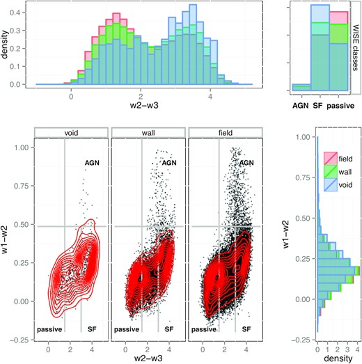
WISE colour–colour diagram and corresponding marginal distributions of (w2−w3) and (w1−w2) colours for galaxies in voids (left scatter plot and blue shadow), walls (middle scatter plot and green shadow), and field (right scatter plot and red shadow). Red lines indicate different isodensity levels, and the grey lines demarcate the regions of the diagram corresponding to the different classes of galaxies which are indicated in the figure. The small upper right-hand panel shows the relative population of the different classes of galaxies in voids (blue), walls (green), and field (red).
Similarly to Figs 1 and 2, the small upper right-hand panel shows the relative population of the different classes of galaxies obtained with the corresponding diagram in voids, walls, and field. Although AGN classified from the WISE diagram are very few, it can be seen a similar behaviour to that obtained with the WHAN diagram, where passive galaxies dominate in the field, and both SF and AGN populate regions of low global density.
As a summary of this section, we present in Table 1 the number of galaxies in the different categories according to the BPT, WHAN, and WISE diagnostic diagram classifications.
4.4 Comparison of diagnostic diagrams
Since AGN emission is associated to accretion on to the massive central black hole, galaxy environment is expected to be correlated to AGN characteristics. This connection may be related to gas rich environments frequent in low and mildly high density regions and where galaxy interactions may play an important role as well.
Following this line, we have investigated possible differences in the classification of AGN comparing the three methods used in this work to select active objects. We also consider the different large-scale environments defined previously. To accomplish this, we have examined the results of the different classification schemes addressed in this work taking into account the environment of the galaxies i.e. voids, walls, or field. We calculate the percentage of galaxies of a given class according to one classification criterium, either BPT, WHAN, or WISE, considering their classification using the other diagnostics tests, i.e. the percentage of cross-classes. The results for void, wall, and field regions are summarized in Table 2. The table is divided into three parts, where the BPT, WHAN, and WISE comparison are displayed in the upper, middle, and lower parts, respectively, as it is indicated in the table. The errors correspond to a Poisson estimate in all cases.
Comparison between AGN diagnostic diagrams for galaxies in voids, walls, and field. Percentages of cross-classes in the different diagnostic diagram used to classified galaxies.
| BPT comparison | |||||||
|---|---|---|---|---|---|---|---|
| BPT class | Large-scale region | WHAN SF | WHAN AGN | WHAN retired/passive | WISE AGN | WISE SF | WISE passive |
| SF | Void | 88 ± 4 | 12 ± 1 | — | 1.2 ± 0.3 | 93 ± 4 | 0.3 ± 0.1 |
| SF | Wall | 85 ± 2 | 15.1 ± 0.5 | 0.02 ± 0.02 | 1.2 ± 0.1 | 92 ± 2 | 0.27 ± 0.05 |
| SF | Field | 86 ± 1 | 14.2 ± 0.3 | 0.08 ± 0.02 | 1.30 ± 0.07 | 92 ± 1 | 0.40 ± 0.04 |
| Composite | Void | 4 ± 1 | 90 ± 10 | 5 ± 1 | 5 ± 1 | 73 ± 8 | 1.7 ± 0.8 |
| Composite | Wall | 3.3 ± 0.4 | 90 ± 4 | 6.5 ± 0.6 | 5.5 ± 0.6 | 71 ± 3 | 2.8 ± 0.4 |
| Composite | Field | 3.3 ± 0.2 | 90 ± 2 | 6.9 ± 0.4 | 5.0 ± 0.3 | 70 ± 2 | 3.8 ± 0.3 |
| AGN | Void | 2 ± 1 | 86 ± 15 | 11 ± 4 | 28 ± 7 | 38 ± 8 | 7 ± 3 |
| AGN | Wall | 1.2 ± 0.3 | 76 ± 5 | 23 ± 2 | 20 ± 2 | 37 ± 3 | 12 ± 1 |
| AGN | Field | 1.1 ± 0.2 | 74 ± 3 | 24 ± 1 | 19 ± 1 | 36 ± 2 | 15 ± 1 |
| WHAN comparison | |||||||
| WHAN class | Large-scale region | BPT SF | BPT composite | BPT AGN | WISE AGN | WISE SF | WISE passive |
| SF | Void | 77 ± 4 | 0.7 ± 0.2 | 0.15 ± 0.09 | 1.3 ± 0.3 | 93 ± 4 | 0.3 ± 0.1 |
| SF | Wall | 73 ± 1 | 0.64 ± 0.07 | 0.11 ± 0.03 | 1.1 ± 0.1 | 92 ± 2 | 0.30 ± 0.05 |
| SF | Field | 72.5 ± 0.8 | 0.63 ± 0.04 | 0.11 ± 0.02 | 1.16 ± 0.06 | 91 ± 1 | 0.42 ± 0.03 |
| AGN | Void | 19 ± 2 | 29 ± 2 | 11 ± 1 | 4.9 ± 0.8 | 76 ± 5 | 0.7 ± 0.3 |
| AGN | Wall | 19.4 ± 0.7 | 26.4 ± 0.8 | 10.3 ± 0.4 | 4.6 ± 0.3 | 76 ± 2 | 1.2 ± 0.1 |
| AGN | Field | 18.0 ± 0.4 | 25.7 ± 0.5 | 10.9 ± 0.3 | 4.6 ± 0.2 | 74 ± 1 | 1.63 ± 0.09 |
| Retired/passive | Void | — | 3.3 ± 0.9 | 2.7 ± 0.8 | 0.2 ± 0.2 | 9 ± 2 | 35 ± 4 |
| Retired/passive | Wall | 0.04 ± 0.03 | 2.6 ± 0.2 | 4.1 ± 0.3 | 0.26 ± 0.07 | 9.7 ± 0.5 | 36 ± 1 |
| Retired/passive | Field | 0.12 ± 0.02 | 2.3 ± 0.1 | 4.2 ± 0.2 | 0.13 ± 0.02 | 9.0 ± 0.3 | 37.4 ± 0.7 |
| WISE comparison | |||||||
| WISE class | Large-scale region | BPT SF | BPT composite | BPT AGN | WHAN SF | WHAN AGN | WHAN Retired/passive |
| SF | Void | 59 ± 3 | 9 ± 1 | 1.8 ± 0.3 | 67 ± 3 | 29 ± 2 | 1.7 ± 0.3 |
| SF | Wall | 54 ± 1 | 9.3 ± 0.3 | 2.2 ± 0.1 | 62 ± 1 | 34 ± 1 | 3.2 ± 0.2 |
| SF | Field | 53 ± 1 | 9.1 ± 0.2 | 2.4 ± 0.1 | 61.6 ± 0.6 | 33.4 ± 0.4 | 3.5 ± 0.1 |
| AGN | Void | 25 ± 8 | 22 ± 7 | 45 ± 12 | 31 ± 9 | 65 ± 16 | 3 ± 2 |
| AGN | Wall | 24 ± 3 | 23 ± 3 | 37 ± 4 | 26 ± 3 | 68 ± 6 | 5 ± 1 |
| AGN | Field | 25 ± 2 | 20 ± 1 | 37 ± 2 | 28 ± 2 | 67 ± 3 | 4.2 ± 0.5 |
| Passive | Void | 4 ± 1 | 3 ± 1 | 2 ± 1 | 5 ± 1 | 7 ± 2 | 34 ± 4 |
| Passive | Wall | 2.4 ± 0.2 | 2.3 ± 0.2 | 2.6 ± 0.2 | 3.4 ± 0.3 | 5.5 ± 0.3 | 35 ± 1 |
| Passive | Field | 2.3 ± 0.1 | 1.9 ± 0.1 | 2.5 ± 0.1 | 3.0 ± 0.1 | 4.9 ± 0.2 | 32.4 ± 0.5 |
For instance, the upper part of the table shows the comparison of BPT SF, composite and AGN galaxies (first column) with WHAN (columns 3-5) and WISE (columns 6-8) categories. In this table, we show the percentages of cross-classes in the different diagnostic diagram. The second column in the table indicates the large-scale region. Notice that the percentages do not add up to 100 due to rounding, and in the case of WISE galaxies there is a set of intermediate objects between SF and passive (1.5 |$\lt (\rm w2-\rm w3)\lt $|3.0) that we have not considered in this analysis. The entries showing and horizontal bar indicate the lack of galaxies of the corresponding class in the large scale region. The middle and lower parts of the table have a similar organization, for WHAN and WISE comparison, respectively. The content of the columns are indicated in their headings.
As it can be seen in the table, there are no significant differences in the AGN fractions according to the large-scale environment in any of the cases analysed. This result suggests that the differences between the classification assigned to each galaxy are related to their criteria and would not be affected by the large-scale environment.
5 AGN ABUNDANCES IN VOID ENVIRONMENT
Here, we analyse the population of active objects in void, wall, and field regions by computing the mean fractions of different galaxy classes in these environments.
The derived relative abundance of AGN according WHAN classification (see Section 4.2) as a function of void radius are given in Fig. 4, where dashed red and long-dashed purple lines correspond to sAGN and wAGN classes, long-dashed green to SF galaxies and solid blue to retired objects. As it can be seen in the left-hand panel of this figure, the fraction of sAGN significantly increases from walls to voids, consistent with a sharp decrease of the fraction of retired galaxies. Moreover, the fraction of sAGN, wAGN, and SF galaxies are all higher in voids, and correspond to a decrease of approximately 60|${{\ \rm per\ cent}}$| of retired galaxies. We also observe that the fraction of SF galaxies monotonically decreases as voidcentric distance increases, in contrast to retired galaxies whose fraction increases with distance. This behaviour is consistent with previous results of galaxy properties in voids (Rojas et al. 2005; Hoyle et al. 2005; Beygu et al. 2017). In the upper right panel of Fig. 4 we show the mean fraction of sAGN to wAGN galaxies. A clear maximum in this relative fraction occurs at void interior and walls. This result is consistent with an increase of the strength of activity in the nucleus in global low-density environments. In the lower right-hand panel of Fig. 4 we show the mean relative fraction of AGN (sAGN + wAGN) to retired galaxies in red lines. As can be seen in the figure, the increment of the relative fraction of AGN to retired as a function of voidcentric distance indicates that AGN galaxies dominate in void interiors. We also show the mean relative fraction of SF to retired galaxies in green lines, which grows towards the voids, as expected according to the well-known properties of galaxies in these environments.
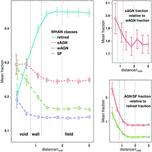
Left-hand panel: Galaxy fractions for different WHAN classes as a function of void-centric distance. Colour and line types correspond to galaxy classes, as is indicated in the figure. Large-scale regions associated with void (field) are indicated by dashed (dotted) black lines. Upper right-hand panel: sAGN fraction relative to wAGN fraction. Lower right-hand panel: AGN (wAGN + sAGN) and SF galaxies fractions relative to retired fraction, in red and green lines, respectively.
In a similar fashion, we have also explored the relative abundance of galaxies classified according to the BPT diagram as a function of the distance to the void centres. The results are shown in Fig. 5 where each colour and line type indicate a class of galaxies; solid red, dashed green, and long-dashed purple lines correspond to AGN, SF, and composite galaxies, respectively. Given the lower number of objects in this sample only one bin was taken in void interiors. The vertical dot lines mark the boundaries between the large-scale low-density regions, namely voids and walls, with the field, and are also indicated in the figure. As can be seen in the figure, the fractions of the three classes of galaxies analysed increase in voids, this result is consistent with those obtained for the SF and AGN galaxies according to the WHAN classification (dashed lines in Fig. 4).
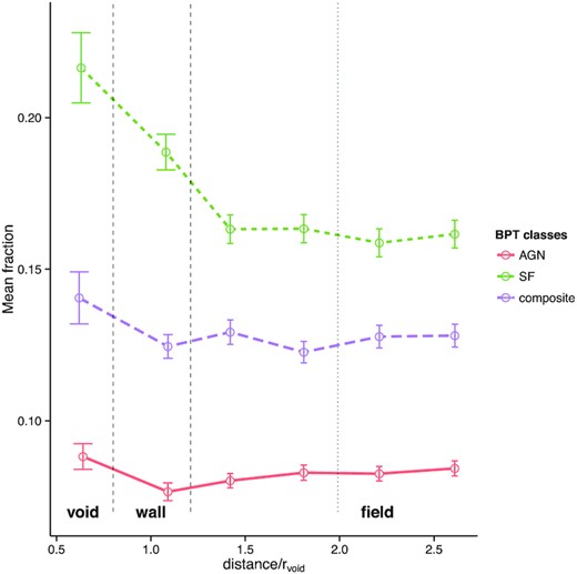
Relative abundance of BPT AGN (solid red line), star-forming (dashed green line) and composite (long-dashed purple line) galaxies, as a function of void-centric distance. Large-scale region limits associated with voids (field) are given by dashed (dotted) black lines.
The fact that WISE AGN may include a significant fraction of obscured AGN could make them suitable to explore environments rich in gas and dust. Accordingly, we have also analysed the relative abundance of galaxies classified according to WISE colours using our environment definition. The resulting fractions of these classes of galaxies as a function of distance to void centres are displayed in Fig. 6. As in Fig. 5, only one bin was taken in void interiors, where it can be seen a significant increase in the fraction of WISE AGN (solid red line) and SF (dashed green line), while a notable decrease is observed in the fraction of passive galaxies in voids (long-dashed blue line).
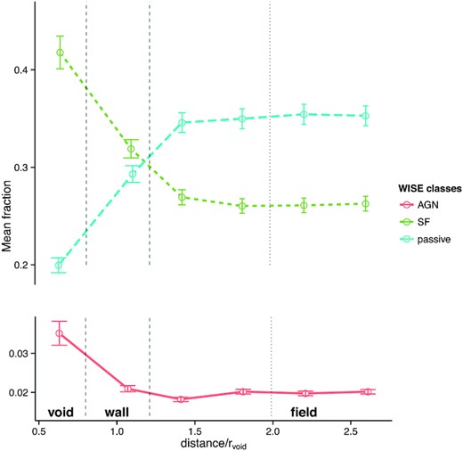
Fractions of WISE AGN (solid red line), SF (dashed green line), and passive (long-dashed blue line) galaxies as a function of void-centric distance. Large-scale region limits associated with voids (field) are given by dashed (dotted) black lines.
The results reported in this section show strong evidence of an increase of the relative population of active galaxies and AGN emission power in voids, this result is independent of the AGN classification scheme for 3 different diagnostic diagrams (Figs 4–6). We want to emphasize that these findings are entirely consistent with the already accepted results regarding the preponderance of galaxies with star–forming activity (Figs 4–6) and the low population of passive galaxies (Figs 4 and 6) in voids.
6 AGN ACTIVITY AROUND VOIDS
In this section, we explore the AGN energy release as inferred by the [O iii] emission-line luminosity (L[O iii]). Also, we analyse EW(H α) line values and black hole mass proxies from correlations with the central stellar velocity dispersion. As in previous sections, we have considered separately void, wall, and field regions.
6.1 The equivalent width of H α
H α emission is related to the number of massive stars and is a direct measurement of the star formation rate. Nevertheless, besides its dependence on star formation activity, the H α luminosity is also affected by AGN activity. For instance, values of EW(H α) are used in WHAN diagrams to separate strong from weak AGN. Moreover, it is also well known that Syfert galaxies have higher values of EW(H α) than LINERs (Cid Fernandes et al. 2010). Taking into account these issues, we have examined the mean EW(H α) values as a function of the distance to voids for both, active and star–forming galaxies classified according to the WHAN diagnostic diagram. The results are shown in Fig. 7(a). As it can be seen in this figure, EW(H α) values increase in voids for sAGN (dashed red line) while on the contrary, they decrease for wAGN (long-dashed purple line). On the other hand, for SF galaxies, no significant dependence are evident (solid green line).
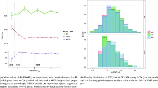
Study of the EW(H α) for the different WHAN classes.
We have also explored the EW(H α) distribution of sAGN and SF galaxies in voids, walls, and field regions, and show the results in Fig. 7(b). The upper panel corresponds to SF galaxies, and the lower panel to sAGN. The line colours correspond to our different definition of large scale environment (blue, green, and red: void, shell and field, respectively). As it can be seen in this figure, the distribution of EW(H α) values for sAGN galaxies in voids differs substantially from that corresponding to wall and field environments (lower panel). This adds to the observed variation of the mean EW(H α) values with voidcentric distance seen in the grey line of Fig. 7(a). On the other hand, the distribution and mean values of EW(H α) for SF galaxies show no significant differences (upper panel of the Fig. 7b). We used the Kolmogorov–Smirnov (KS) test to evaluate the statistical significance of the differences between EW(H α) distributions for different large-scale environments. If the p–value is less than 0.05, we consider that the differences between distributions are highly significant. Since p-values obtained for SF galaxies are larger than 0.6, according to this test, the difference between the samples is not significant enough to confirm that they have different distribution. On the other hand, we obtain p-values < 0.01 for sAGN samples in voids and field, and in voids and walls. This confirms that the differences in the EW(H α) distributions are significant, whereas for wall and field sAGN the resulting p-values is greater than 0.01 indicating that the two samples come from the same distribution.
The median (mean) logarithmic values of the EW(H α) distributions of SF and sAGN galaxies in voids yield values 1.18 (1.22) and 1.15 (1.19), respectively. These results show evidence of higher EW(H α) values for star-forming galaxies than for AGN in void environment, consistent with the overall larger star formation activity characterizing these regions. However, if we compare to field galaxies, we obtain that the ratio between the medians of the log EW(H α) distributions for sAGN and SF galaxies are 0.062 and 0.013, respectively. This result indicates that the Hα equivalent widths of sAGN are significantly more affected by the void large-scale environment.
In WHAN star-forming galaxies, although their relative population in voids increases (long-dashed green line in Fig. 4), their Hα equivalent widths remain approximately constant in different large-scale regions (solid green line in Fig. 7a). Nevertheless, we find higher fractions and a noticeable increment of H α equivalent widths for WHAN sAGN (dashed red lines in Figs 4 and 7a), consistent to an increment of AGN activity in voids. This behaviour, which seems to be characteristic of active galaxies, could account for the effects of the global environment defined by voids in destabilizing the central regions of the galaxies.
6.2 The [O iii] luminosity
The [O iii] luminosity (L[O iii]) is considered a suitable proxy of the AGN activity. Although this line is also suitable to trace for the presence of massive stars, it is relatively weak in star-forming galaxies which are rich in metals (Kauffmann et al. 2003; Heckman et al. 2004). An advantage of using the [O iii] line is its strength and the fact that it can be easily detected in most galaxies. In this work, we use the [O iii] line corrected for optical reddening using the Balmer decrement and the obscuration curve of Calzetti et al. (2000).
We study the [O iii] luminosity of BPT AGN populating void, wall and field regions. To analyse this we examine the distribution of L[O iii] for AGN galaxies in voids, walls and field that is represented in the upper panel of the Fig. 8(b). Each colour corresponds to a different large-scale region as indicated in the figure. As can be seen, the distributions are remarkably different. The statistical significance of these differences is reinforced with the p-values obtained from the KS test, which are less than 0.05.
![Study of the [O iii] luminosity for the BPT AGN.](https://oup.silverchair-cdn.com/oup/backfile/Content_public/Journal/mnras/509/2/10.1093_mnras_stab2902/1/m_stab2902fig8.jpeg?Expires=1750307629&Signature=BTUnH7iJbRIE8zRFoItHkXkgJ3NrQUBlx8psJYP-2xaRX-Wlh3BWXyWjjFdZNHCpqZDtAnunUM2DflRLvSowR1hLDv57rMp0X9VwF9UW~YWJaS1ABgq6hJSxrMohELRztYl7JO6kMDXtmxjVSoF4nHwycd98D3GrCHemUpo11WRj4CEM53eYnGftGJTfWmdjZmWiA-Sh4lkzzAqzfV-lmknW5TDBVOgB0p35BoCM6mtKMUjsP-0xHOaEI5p3n9V76f7kx-wuBfYdySL5Za5NfPu865m3DW0eukv05yYfIIqPI1~dRYylhvUKSwVzysvkbEwsTWFFZgZh3wkaU8MZ6w__&Key-Pair-Id=APKAIE5G5CRDK6RD3PGA)
Study of the [O iii] luminosity for the BPT AGN.
We have considered sub-samples selected according to percentiles in the distribution of black-hole mass proxy, and in Fig. 8(b), we show the distribution of L[O iii] for BPT AGN in void, wall and field environments with BH mass greater than percentiles 25, 50, 75, 80, and 90 (i.e. log(MBH/|$\rm M_\odot$|) ≥ 7.29, 7.64, 8.03, 8.15, and 8.45, respectively). The upper panels provide the results of wall regions (green), and the lower panels void (blue) environments. In both cases, the field region (red) is shown for comparison. Black hole mass percentiles are indicated in the upper labels. As it can be seen, for all cases, AGN in voids and walls exhibit larger L[O iii] values than their field counterparts.
In order to study the dependence of the [O iii] luminosity on voidcentric distance, we show in Fig. 8(a) the mean L[O iii] values for different lower thresholds of BH mass proxy (those associated to the previously adopted BH mass percentiles namely |$\rm log(M_{\rm BH}/M_{\odot }) \ge$| 7.29, 7.64, 8.03, 8.15, and 8.45, corresponding to the 25, 50, 75, 80, and 90 percentiles, respectively). In this figure, these BH mass lower limits are shown in different colour intensity, and the darkest one represents the full AGN sample. From this figure, it can be seen that AGN in void regions exhibit the largest L[O iii] values, whereas the smaller ones are found in the field. Moreover, there is a significant increase in L[O iii] mean values in void regions as reflected in the higher values as the distance to the void decreases. This is observed for all BH mass thresholds although it is more noticeable for the most massive BHs (p75, p80, 90, the 3 lighter lines in the figure). We notice that due to the low number of AGN in voids, we have only considered one bin within the void radius.
Since according to WHAN classification, sAGN dominate over wAGN in voids (see right-hand upper panel of Fig. 4), we have selected BPT AGN with high [O iii] luminosity to further explore this effect. Our procedure follows the use of L[O iii] as a tracer of the strength of nuclear activity and adopt the criterium that the most powerful AGN are those with L[O iii] > 107 L⊙. A similar limit has been adopted previously by several authors to select powerful AGN (e.g. Kauffmann et al. 2003; Coldwell et al. 2009; Alonso, Coldwell & Lambas 2013; Duplancic et al. 2021). We study the population of powerful AGN by analysing their relative fraction as a function of voidcentric distance. The results are portrayed in Fig. 9, where each colour corresponds to different lower limits of BH mass associated to the same percentiles as in Fig. 8(a). Similarly, the result for the full AGN sample is shown in the darkest line of Fig. 9, and we only considered one bin within the void radius due to the low number of AGN in voids in each subsample. As it can be seen in this figure, there is a relevant population of powerful AGN in void regions since the fraction of high L[O iii] values increases towards void centres. Moreover, this trend is more noticeable for the most massive BH subsamples (per centiles 75, 80, 90).
![Relative abundance of BPT AGN with high [O iii] luminosity as a function of voidcentric distance for different black-hole mass thresholds ($\rm log(M_{\rm BH}/M_{\odot })\ge$ 7.29, 7.64, 8.03, 8.15, and 8.45, associated with the 25, 50, 75, 80, and 90 percentiles, respectively). Black-hole mass increases for lighter colours as indicated in the figure. Large-scale regions associated with voids (field) are indicated by dashed (dotted) black lines.](https://oup.silverchair-cdn.com/oup/backfile/Content_public/Journal/mnras/509/2/10.1093_mnras_stab2902/1/m_stab2902fig9.jpeg?Expires=1750307629&Signature=tQ4zqTadLKYhnnLneWlJTyNk1aWVy89p7vpUigcDGrMvGoWpwFSt9Nvlx3M3y0Ep6wP3Ak1E1NefEuHpHEdmsrRwu8V9IbDs8SOUIgTY0NlUKgGZ0ijIX1bzblPxxGaehWdK6UH3glNG9fLpxg25Dm7v4nNCoxBOVkavpb~LDQfiy6H7aHSmP7trvcL3KN4V2nCgj2981kjaqDbjvTJzX9xNrLAbp9WGNsBtfvrfdDUhHA8bh-fdK0zUUsGa8lY8g7fVHFkov8F3JULaSPUNIHSYZKQp1r4Pxm9lZs2QnT5cMcE6y6JguPS1uyVckz5~vSRXcvwNbODTVdVhCaOrsg__&Key-Pair-Id=APKAIE5G5CRDK6RD3PGA)
Relative abundance of BPT AGN with high [O iii] luminosity as a function of voidcentric distance for different black-hole mass thresholds (|$\rm log(M_{\rm BH}/M_{\odot })\ge$| 7.29, 7.64, 8.03, 8.15, and 8.45, associated with the 25, 50, 75, 80, and 90 percentiles, respectively). Black-hole mass increases for lighter colours as indicated in the figure. Large-scale regions associated with voids (field) are indicated by dashed (dotted) black lines.
We have also explored samples of AGN selected in the infrared provided by WISE. Since several Optical BPT AGN are also identified as mid-IR active objects by using WISE colour–colour diagram, here we explore what is the role of these galaxies in void regions and analyse their influence in the peak of the L[O iii] distribution. The resulting distributions are displayed in the upper panel of Fig. 10, where we show the L[O iii] distribution of AGN selected by both WISE and BPT criteria (yellow). As it can be seen, the distributions look similar in void, wall and field, their median values are indistinguishable as well (p-values from KS test are > 0.2 for all combination of subsamples). We also display the L[O iii] of BPT AGN in black lines (notice that these distributions are already shown in the in upper panel of Fig. 8(b) and are displayed here to facilitate comparisons). As it can be noticed, AGN WISE selection is preferentially associated to powerful optical AGN in all environments examined here (appropriately, 80 per cent have L[O iii]>107 L⊙).
![Upper panel: Normalized distribution of the [O iii] luminosity for BPT AGN which are also classified as AGN following WISE (yellow) and WHAN (green) criteria. Black lines shows the L[O iii] distribution for BPT AGN. Each panel indicates galaxies in void, wall and field regions. Bottom panel: Scatter plots of the black hole mass estimates versus L[O iii] for AGN in voids, walls and field, with marginal distributions for black hole mass estimates. The different colours correspond to AGN selection criteria as in the upper panel.](https://oup.silverchair-cdn.com/oup/backfile/Content_public/Journal/mnras/509/2/10.1093_mnras_stab2902/1/m_stab2902fig10.jpeg?Expires=1750307629&Signature=P-uP30RUteY9gagzRgC5bE4Ji3PKKBJfHZK5NOMOskCdqQYwdkWB0v9k3f9~ZEDLky4LjKy8gOtwtpFGROoa5Nq7LyR2FEdia~et9SCt7Y5MvAG5-lvHdNadpCOT~cT4mzkqdXJ~LkS-ORC7jvd56Rtt0DyRlAufgSnbmrcm4qF82j~N8X~OJBy9-JL-YDDsnFYLTi9wSuUFOJTJLJqB6OrKZZ3TDtpcp9ROzulB3A8dF8jCGZrIuub-xkAMgmruX61FiW20WD9y5BRoWlnKjPrjQeRxir8XBiSUat60lVHv488RecVI1nLtdMhARZsoEpqkE8SDEJiOQA3SGFYlDg__&Key-Pair-Id=APKAIE5G5CRDK6RD3PGA)
Upper panel: Normalized distribution of the [O iii] luminosity for BPT AGN which are also classified as AGN following WISE (yellow) and WHAN (green) criteria. Black lines shows the L[O iii] distribution for BPT AGN. Each panel indicates galaxies in void, wall and field regions. Bottom panel: Scatter plots of the black hole mass estimates versus L[O iii] for AGN in voids, walls and field, with marginal distributions for black hole mass estimates. The different colours correspond to AGN selection criteria as in the upper panel.
Additionally, for comparison we have explored the contribution of WHAN sAGN to the L[O iii] distribution in voids, walls and field. We consider sAGN that are also classified as active objects by BPT. The results are displayed in green in the upper panel of Fig. 10. As expected WHAN sAGN are also associates with powerful AGN-selected according to their [O iii] luminosity (the percentage of galaxies with L[O iii]>107 L⊙ ranges from 70–80 per cent when going from field to void). As can be easily seen in the figure, WISE AGNs are the most powerful objects in general, regardless of the global environments analysed here. None the less, when we examine the galaxies in voids, we obtain a remarkable fraction of powerful AGN, whose value (L[O iii]>107 L⊙ fraction ∼ 0.8) is similar for any of the criteria adopted to select them. Furthermore, the [O iii] luminosity distributions of the AGN subsamples presented in the figure are comparable both in means and in dispersion when they are in voids, unlike what we obtain when these galaxies reside in walls and field.
We have also analysed the relations between BH mass estimates and [O iii] luminosity for AGN in voids, walls and field, which are displayed in scatter plots in the lower panels of Fig. 10. We have studied subsamples of AGN selected according to the BPT criteria (black points), BTP that are also WISE AGN (yellow points) and WHAN sAGN also active according to the BPT diagnostic diagram (green points), similarly to what was done in the upper panel of this figure. We also show the corresponding marginal distributions of BH mass estimates in the vertical right-hand panels. From this figure, it can be appreciated a slight correlation between BH mass and L[O iii] for WISE and WHAN subsamples (yellow and green points), moreover WISE AGN seems to be associated not only to the most powerful objects but also to galaxies with larger BH mass, especially for wall and field galaxies.
Based on the previous results, it is interesting to study the accretion strength of the central black holes. To this end, we calculate the accretion rate parameter, |$\cal R=\rm log(\rm L[O\, {\small III}]/M_{\rm BH})$| (Heckman et al. 2004), that provides a widely used estimate of the AGN efficiency. We explore this efficiency parameter as a function of voidcentric distance for the AGN subsamples described in Fig. 10 and show the results in Fig. 11. From this analysis, we show that WISE AGN and WHAN sAGN exhibit a higher fraction of efficient accretion rate with respect to the BPT AGN. This trend is independent of the large-scale environment. Moreover there is an increment in the mean accretion rate with decreasing voidcentric distance and in void interiors WISE AGN display the higher |$\cal R$| values in comparison with active galaxies selected according to BPT and WHAN.
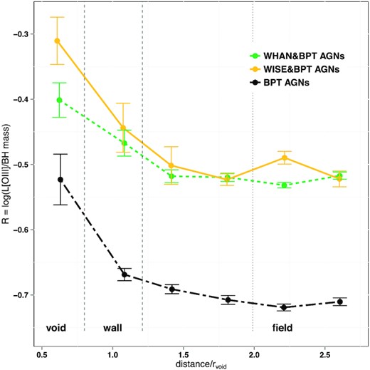
AGN efficiency in void, wall and field, for galaxies satisfying the AGN classification criteria of WHAN and BPT (dashed green line), WISE and WHAN (solid yellow line), and BPT (two-dashed black line).
Alonso et al. (2018) study the influence of bars and interaction on AGN properties. These authors select galaxies with high accretion rate considering |$\cal R$| > −0.6 and found that barred AGN galaxies show a moderate excess of efficient accretion rate with respect to active galaxies in pairs and in a control sample. In this work, we find that within voids AGN have |$\cal R$| mean values well above this threshold. Moreover all BPT active galaxies also selected as AGN by WISE or as sAGN by WHAN are high accreting objects.
7 SUMMARY AND RESULTS
In this work, we identify star-forming AGN and passive galaxies in an SDSS volume-limited galaxy sample and study the influence of large-scale environment by considering the distance to cosmic voids centres. We use BPT and WHAN optical line diagnostic diagrams as well as mid-IR colour–colour diagrams based on WISE data. By following this approach, we can perform a detailed analysis of the physical characteristics of active galaxies in an homogeneously identified samples of voids.
The main results of this work can be summarized in the following items:
An increment of both star-forming and AGN galaxies from walls towards void interiors, compared with field regions. These trends are independent of the classification schema and are evident for WHAN, BPT, and WISE star-forming and active objects identification criteria.
Decreasing fraction of WHAN and WISE passive objects from field towards void interiors. This is consistent with a lack of passive galaxies in underdense regions.
An increment of the H α equivalent widths of WHAN sAGN towards void regions consistent with more powerful objects associated to void environments.
We find that BPT AGN in void regions show higher L[O iii] values for similar black hole mass ranges with a tendency for [O iii] luminosities to increase with |$\rm {\it M}_{\rm BH}$|. Therefore, we expect AGN residing in voids to have larger [O iii] luminosity than counterparts with similar black hole masses located in a global density environment.
WISE AGN also selected as optical active objects have the highest [O iii] luminosities regardless their large-scale environment. Moreover, these AGN correspond to those with the highest accretion rate (|$\cal R \gt $|−0.6) in our analysis. These effects become stronger within the void environment.
We further notice that examining these topics could help to better understand the role of the different accretion mechanisms that trigger nuclear activity in galaxies. Overall, AGN feeding mechanisms are expected to be effective in local underdense regions that are rich in gas, part of which can be efficiently conducted to the central regions of galaxies via radiative cooling. This mechanism could become a suitable source for accretion on to the center of galaxies and feed galactic nuclei (Davies & Lewis 1973; Solanes et al. 2001; di Serego Alighieri et al. 2007; Grossi et al. 2009; Cortese et al. 2011; Catinella et al. 2013). This scenario could be key to explain our findings of a larger fraction of AGN in voids and walls which are gas rich, locally underdense regions, with additional fuel by gas expanding from void interiors.
8 DISCUSSION AND CONSLUSIONS
The void underdense environment provides a simpler dynamical behaviour compared to that of groups and clusters. For this reason, it is relevant to explore the possible effect of these environments on galaxy evolution, particularly star formation and central AGN accretion. In this context, nuclear activity in galaxy hosts residing in voids and surrounding regions can be important to understand the interplay between star formation and black hole accretion and the role of environment. The presence of AGN in cosmic voids had been reported by different authors (Constantin et al. 2008; Liu et al. 2015; Argudo-Fernández et al. 2018). Nevertheless the influence of large-scale environment on AGN activity is still on debate. Amiri et al. (2019) used volume-limited samples of galaxies to compare the fraction of AGN in rich galaxy clusters and voids finding that in the local Universe (0.01 < z < 0.04) AGN activity has a larger dependence on host stellar mass than on the local galaxy density. In the same line Miraghaei (2020) also find small effects of environment on AGN activity although it is reported a higher fraction of optical AGN in massive red galaxies in voids compared to similar galaxies in dense environments. On the theoretical side, using cosmological hydrodynamical simulations Habouzit et al. (2020) find a coeval evolution of galaxies in voids and their central black holes, where an approximately 20 per cent of them become AGNs.
In this work, we have study the relative fraction of galaxies with different activity classes as a function of distance to cosmic voids centres. In order to analyse, the activity of galaxies we use the BPT, WHAN, and WISE diagrams in a volume limited sample of galaxies extracted from the SDSS. Briefly, our results show a predominance of actively star-forming galaxies and an clear excess of AGN galaxies inside voids and in void surroundings. This result is independent of the classification scheme addressed (either BPT, WHAN, or WISE). The increment of the fraction of AGN and star-forming galaxies is evident from walls to void interiors. We also notice that although void walls correspond to the boundaries of cosmic voids, given our relatively strict void definition, these edges are regions still largely underdense in global expansion with respect to void centres. In this line, we recall previous studies of the effect of the large-scale environment in walls surrounding voids as reported by Ceccarelli et al. (2008, 2012).
We detected a significant deficit of retired and passive galaxies in voids when we studied the WHAN and WISE classifications. This behaviour is consistent with the expected properties of galaxies in low-density regions. This result, combined with the increase of the population of star-forming galaxies in voids, constitutes a further confirmation of the well-studied properties of void galaxies.
A relevant issue concerning our results on AGN activity and the location of hosts with respect to void centres is the tendency of AGN galaxies to populate preferentially voids and walls rather than the field regions. This could be related to the fact that hosts residing these environments may have their central black hole accretion rate fuelled by gas flowing from void interior outwards the void. On the other hand in high-density regions as the centres of galaxy clusters or rich groups it has been show a lack of AGN excess (e.g. Popesso & Biviano 2006; Coldwell et al. 2014, 2017; Amiri et al. 2019). This may be a consequence of low merging rate given the high-velocity dispersion of these systems and also the interaction with cluster hot gas that may cause a depletion of gas from galaxies. Note that the global low-density environment is uniquely characterized by voids, while active galaxies have different selection criteria. It is, therefore, interesting to examine whether the environment is reflected in different ways with different selection criteria. To analyse this, we use three different schemes to classify and select AGNs and we obtain consistent results with all of them, giving extra strength to the results. It is worth mentioning that although we use two methods based on the optical (BPT and WHAN), the third method based on mid-IR (WISE) is different and confirms and reinforces our results.
The fact that AGN dominate in void interiors and walls could serve to obtain well-traced voids in large cosmological volumes. This could be important not only for void statistics and galaxy evolution, which is itself interesting, but also for cosmological applications such as the AP test. Taking into account the upcoming new generation of galaxy surveys, these results can be relevant for several large-scale studies.
ACKNOWLEDGEMENTS
This work has been partially supported by Consejo de Investigaciones Científicas y Técnicas de la República Argentina (CONICET), the Secretaría de Ciencia y Técnica de la Universidad Nacional de Córdoba (SeCyT), and Secretaría de Ciencia y Técnica de la Universidad Nacional de San Juan. Funding for the SDSS and SDSS-II has been provided by the Alfred P. Sloan Foundation, the Participating Institutions, the National Science Foundation, the U.S. Department of Energy, the National Aeronautics and Space Administration, the Japanese Monbukagakusho, the Max Planck Society, and the Higher Education Funding Council for England. The SDSS web site is http://www.sdss.org/. The SDSS is managed by the Astrophysical Research Consortium for the Participating Institutions. The Participating Institutions are the American Museum of Natural History, Astrophysical Institute Potsdam, University of Basel, University of Cambridge, Case Western Reserve University, University of Chicago, Drexel University, Fermilab, the Institute for Advanced Study, the Japan Participation Group, Johns Hopkins University, the Joint Institute for Nuclear Astrophysics, the Kavli Institute for Particle Astrophysics and Cosmology, the Korean Scientist Group, the Chinese Academy of Sciences (LAMOST), Los Alamos National Laboratory, the Max-Planck-Institute for Astronomy (MPIA), the Max-Planck-Institute for Astrophysics (MPA), New Mexico State University, Ohio State University, University of Pittsburgh, University of Portsmouth, Princeton University, the United States Naval Observatory, and the University of Washington. This research has used the NASA’s Astrophysics Data System. Plots were performed using R software.
DATA AVAILABILITY
The data underlying this article will be shared on reasonable request to the corresponding author.
Footnotes
Available in CAS galSpecIndx, galSpecInfo, galSpecLine and galSpecExtra tables.
The cross-matched WISE data is available in CAS WISE_allsky and WISE_xmatch tables.
