


ABSTRACT
We study differential rotation in late-stage shell convection in a 3D hydrodynamic simulation of a rapidly rotating |$16\, {\rm M}_{\odot }$| helium star with a particular focus on the convective oxygen shell. We find that the oxygen shell develops a quasi-stationary pattern of differential rotation that is described neither by uniform angular velocity as assumed in current stellar evolution models of supernova progenitors, nor by uniform specific angular momentum. Instead, the oxygen shell develops a positive angular velocity gradient with faster rotation at the equator than at the pole by tens of per cent. We show that the angular momentum transport inside the convection zone is not adequately captured by a diffusive mixing-length flux proportional to the angular velocity or angular momentum gradient. Zonal flow averages reveal stable large-scale meridional flow and an entropy deficit near the equator that mirrors the patterns in the angular velocity. The structure of the flow is reminiscent of simulations of stellar surface convection zones and the differential rotation of the Sun, suggesting that similar effects are involved; future simulations will need to address in more detail how the interplay of buoyancy, inertial forces, and turbulent stresses shapes differential rotation during late-stage convection in massive stars. If convective regions develop positive angular velocity gradients, angular momentum could be shuffled out of the core region more efficiently, potentially making the formation of millisecond magnetars more difficult. Our findings have implications for neutron star birth spin periods and supernova explosion scenarios that involve rapid core rotation.
1 INTRODUCTION
Stellar rotation is a key factor in the evolution of massive stars (Maeder & Meynet 2000; Langer 2012). Reliable modelling of the rotational evolution of massive stars, which is determined by internal angular momentum transport, wind mass-loss, and binary interactions, is essential for understanding the spins of neutron stars and black holes, and the role of rotation in the supernova explosion mechanism. Accurate knowledge of the presupernova distribution of angular momentum is particularly important in the context of extremely energetic ‘hypernovae’ and long gamma-ray bursts that may be produced by rapidly rotating ‘millisecond magnetars’ (Duncan & Thompson 1992; Thompson & Duncan 1993; Akiyama et al. 2003) or by black hole accretion discs in the collapsar scenario (Woosley 1993; MacFadyen & Woosley 1999). The problem of angular momentum transport in stellar interior is intimately connected with the theory of stellar dynamos (Brandenburg & Subramanian 2005; Charbonneau 2014) and with the observed diversity of neutron star magnetic fields from |$10^{10}\,\,\text {to}\,\,10^{13}\, \mathrm{G}$| in normal pulsars to |${\sim } 10^{15}\, \mathrm{G}$| in observed magnetars, which yet awaits an explanation (Olausen & Kaspi 2014; Kaspi & Beloborodov 2017). Dynamo-generated fields will influence the rotational evolution of massive stars up to core collapse (Spruit 2002; Heger, Woosley & Spruit 2005; Fuller, Piro & Jermyn 2019). Conversely, the rotational evolution of massive stars will have a bearing on the magnetic fields of neutron stars, whether these are set by the precollapse field via flux conservation (Ferrario & Wickramasinghe 2006) or generated after collapse by dynamo action (Thompson & Duncan 1993).
Current stellar evolution models of supernova progenitors can treat rotation in a ‘1.5D-approach’ that assumes shellular rotation and includes angular momentum transport processes by means of appropriate diffusion and/or advection terms (Heger, Langer & Woosley 2000; Meynet & Maeder 2000; Heger et al. 2005).1 State-of-the-art models (Heger et al. 2000, 2005) account for a range of mixing processes, including the dynamical and secular shear instability (Endal & Sofia 1976), the Solberg–Høiland instability (Wasiutynski 1946), meridional circulation (Eddington 1926; Kippenhahn 1974; Chaboyer & Zahn 1992; Zahn 1992), the Goldreich–Schubert–Fricke instability (Goldreich & Schubert 1967; Fricke 1968), and magnetic stresses generated by the Tayler–Spruit dynamo (Spruit 2002). Within convective zones, the diffusion coefficient for angular moment is constructed from the turbulent velocity and correlation length, which can be estimated using mixing-length theory (MLT; Böhm-Vitense 1958). It is usually assumed that the diffusive terms drive the angular momentum distribution towards uniform rotation, consistent with the notion that this represents the asymptotic state of thermodynamic equilibrium (Landau & Lifshitz 1969). Specifically, rigid rotation is established within convective regions within a few turnover times in current diffusion-based approximations for angular momentum transport.
There are abundant indications, however, that current recipes for angular momentum transport in stellar evolution models require further refinement. For example, more efficient angular momentum transport is required to account for asteroseismic measurements of low-mass stars (Cantiello et al. 2014; Aerts, Mathis & Rogers 2019). What is most interesting among the observational findings in the context of this study, though, are indications that convective zones do not evolve towards rigid rotation. Helioseismology reveals that the Sun’s convective zone rotates |${\sim } 34 {{\ \rm per\ cent}}$| faster at the equator than near the poles (|$470\, \mathrm{nHz}$| versus |$350\, \mathrm{nHz}$|; Howe 2009). Similar findings have been obtained for a few dozen solar-like stars via asteroseismology (Benomar et al. 2018), e.g. HD 173701 rotates twice as fast at the equator as near the pole.
The emergence of differential rotation is not entirely unexpected, and various ideas have been proposed to account for it. It has long been recognized that meridional circulation, if properly modelled, can build up differential rotation (Maeder & Zahn 1998; Eggenberger, Maeder & Meynet 2005). In the context of the Sun, attempts have been made to explain the angular momentum distribution in the convection zone based on simple hydrodynamic principles by invoking thermal wind balance (Kitchatinov & Ruediger 1995; Balbus et al. 2009). Extending these ideas, Jermyn et al. (2020a, b) recently proposed scaling laws for differential rotation in convective regions, which agree qualitatively with global hydrodynamic and magnetohydrodynamic simulations of stellar surface convection zones (e.g. Käpylä et al. 2011; Mabuchi, Masada & Kageyama 2015) and rotation profiles determined via asteroseismology. According to Jermyn et al. (2020a, b), convective zones are expected to develop strong differential rotation in the case of high Rossby number (slow rotation) and asymptote to rigid rotation in the limit of small Rossby number (rapid rotation).
While 1D stellar modelling based on the mixing-length theory of convection (Böhm-Vitense 1958), with appropriate generalizations for the transport of composition and angular momentum by other instabilities (e.g. Heger et al. 2000, 2005; Maeder et al. 2013) remain the state of the art for stellar evolution calculations over secular time scales, multidimensional simulations have opened a new window on mixing and angular momentum in stellar interiors. There is already a long history of simulations that have addressed the rotation of the solar convection zone and the surface convection zones of other stars (e.g. Brun, Miesch & Toomre 2004; Käpylä et al. 2011; Matt et al. 2011; Guerrero et al. 2013; Mabuchi et al. 2015; Robinson, Tanner & Basu 2020; and Charbonneau 2014 for a review). Despite a recent surge in in 3D simulations of late-stage convective burning (Meakin & Arnett 2007; Müller et al. 2016; Cristini et al. 2017; Jones et al. 2017; Fields & Couch 2020; McNeill & Müller 2020; Yadav et al. 2020; Varma & Müller 2021; Yoshida et al. 2021a), the interplay of convection and rotation has not yet been thoroughly explored by means of multidimensional hydrodynamic models during the late convective burning stages, despite possible implications for the spins and magnetic fields of neutron stars and supernova explosion physics. Due to the physical differences between the regimes of surface convection zone and late-stage convective burning (where radiative diffusion is completely unimportant), it is not clear whether the findings of the former can be translated directly to the interiors of massive stars. The problem of convection in rotating massive stars was only touched in passing by Kuhlen, Woosley & Glatzmaier (2003) using anelastic 3D simulations with simplified source terms for nuclear burning. Subsequent studies of convection in late-stage burning shells of rotating progenitors by Arnett & Meakin (2010) and Chatzopoulos et al. (2016) were limited to axisymmetry (2D). Remarkably, Arnett & Meakin (2010) found that the convective shell adjusted to constant specific angular momentum, which can be motivated by marginal stability analysis based on the Rayleigh criterion. This would be in stark contrast to the assumption of uniform rotation within convective zone in 1D stellar evolution models, and might seriously impact the secular evolution of the angular momentum profiles of massive stars on their way to core collapse. The assumption of axisymmetry, however, places a major caveat on these results. Recently, Yoshida et al. (2021b) presented a short 3D simulation covering |$91.6\, \mathrm{s}$| of oxygen shell burning in a rapidly rotating supernova progenitor, which showed adjustment towards constant specific angular momentum in the convective region. If confirmed, evolution towards constant specific angular momentum in convective zone might significantly alter the rotation profiles of massive stars compared to current 1D stellar evolution models, making it easier to maintain fast rotation in the stellar core region. This would be especially important in the context of progenitor scenarios for magnetorotational supernova explosions powered by ‘millisecond magnetars’ (Usov 1992; Duncan & Thompson 1992; Akiyama et al. 2003). However, the short simulation time of Yoshida et al. (2021b) calls for a closer look in longer simulations to confirm possible deviations from solid-body rotation in the inner convective zones of massive stars.
Here, we investigate the question of differential rotation in rapidly rotating convective regions (i.e. with rotational velocities exceeding convective velocities) during oxygen burning for the first time in 3D, with a view to corroborating or improving stellar evolution models of massive stars, and with an eye to the possible implications for core-collapse supernovae and neutron stars. We perform a full 4π solid angle simulation of the shells around the iron core in a rapidly rotating |$16\, {\rm M}_{\odot }$| helium star from a series of gamma-ray burst progenitor models by Woosley & Heger (2006). We evolve the model for 12 min, or about 30 convective turnover times in the oxygen burning shell. Using spherically averaged 1D profiles, an analysis of 2D zonal averages, and a spherical harmonics analysis, we attempt to better define the preferred rotation state in the convective region. We interpret our results in the light of proposed theories for differential rotation in convective zones and discuss implications for stellar evolution calculations.
Our paper is structured as follows: In Section 2, we briefly review theoretical arguments about the angular momentum distribution in convective zones. In Section 3, we describe the numerical methods and the set-up of our 3D model. In Section 4, we analyse the differential rotation in our simulation using 1D and 2D flow decomposition, and discuss possible physical mechanisms for the unexpected angular momentum distribution, which evolves neither towards uniform specific angular momentum nor towards uniform angular velocity. In Section 5, we summarize our findings and discuss possible implications for the evolution of massive stars and supernova scenarios involving rapid progenitor rotation.
2 BRIEF REVIEW OF ARGUMENTS ON THE ROTATIONAL STATE OF CONVECTIVE ZONES
Before discussing our simulation results, it is useful to briefly review key arguments that have hitherto been used to support or criticize the assumption of uniform rotation in convective regions in evolutionary models of massive stars.
2.1 Angular momentum distribution in convective regions
As the simplest argument for uniform rotation in convective zones, one might invoke the principle that only uniform rotation is allowed in thermodynamic equilibrium (Landau & Lifshitz 1969). For a given amount of angular momentum in a closed system, dissipation will ultimately drive the system towards uniform rotation as the state of minimal free rotational energy, which permits no further dissipation by viscous forces. This argument is specious, however, since stellar convection zones are open non-equilibrium systems, and must actually be continuously driven away from thermodynamic equilibrium (by nuclear burning, neutrino cooling, or radiative/conductive heat transport to the surrounding shells) to maintain steady-state convection. Such systems will often settle into a quasi-equilibrium state, but this quasi-equilibrium is determined by dynamical considerations and does not necessarily resemble the thermodynamic equilibrium state, e.g. the non-isothermal stratification of convection zone and excited eccentricity in tidally interacting binaries (McNeill, Mardling & Müller 2020).
It has been argued that uniform rotation should indeed arise as such a dynamical quasi-equilibrium. The key idea is that horizontal shear is generally quickly eliminated by efficient turbulent angular momentum transport to enforce ‘shellular rotation’ (Zahn 1992), and that in convective zones efficient angular momentum transport by dynamical shear instability (Zahn 1974) also eliminates vertical shear, so that the convective zone adjusts to a marginally stable state in which shear does not drive any further angular momentum transport on dynamical time scales. Essentially, this argument already goes back to Endal & Sofia (1976), who appealed to the effective turbulent viscosity provided by convective motions to enforce a state of marginal stability.
In addition to the inertial and buoyancy forces determined by the large-scale, temporally and spatially averaged flow, turbulent stresses can also affect the force balance and destroy uniform rotation by ‘antidiffusive’ transport of angular momentum by the Λ-effect (Krause & Rüdiger 1974; Ruediger 1989; Kichatinov & Rüdiger 1993). In reality, both effects may play a role, and their relative contribution is still under debate in the case of the Sun (e.g. Brun, Antia & Chitre 2010).
2.2 Relation to 1D mixing length theory
In the subsequent discussion, we shall evaluate these considerations in the context of late-stage convection in massive stars using our 3D hydrodynamics simulation.
3 SHELL BURNING SIMULATION
We have performed a 3D simulation of convective shell burning of model HE16O from Woosley & Heger (2006). This model is a rotating |$16 \, {\rm M}_{\odot }$| helium star with a rotational velocity that is of order of a few per cent of the Keplerian velocity in the oxygen shell, and similar to the convective velocities, i.e. the convective Rossby number is of order unity. The stellar evolution model assumes shellular rotation and includes angular momentum transport by hydrodynamic processes and magnetic torques following Heger et al. (2000, 2005).
Following the methodology of Müller et al. (2016), we map the 1D stellar evolution model into the finite-volume code prometheus (Fryxell, Müller & Arnett 1989; Fryxell, Arnett & Mueller 1991) at a late pre-collapse stage about 12 min before the onset of collapse. We then follow the evolution to the onset of collapse, contracting the inner boundary following the trajectory of the corresponding mass shell in the stellar evolution model. Our simulation includes the mass shells initially located between |$3800$| and |$31\,200\, \mathrm{km}$|, which covers three distinct convective burning shells. These are shown as shaded cyan regions in the progenitor entropy profile in Fig. 1, indicated by the three flat entropy gradients located around 4200, 7000, and |$9000\, \mathrm{km}$|, corresponding to oxygen burning, neon burning, and carbon burning, respectively. We shall mostly focus on the oxygen shell, which undergoes about 13 turnovers over the period of interest (and about 26 for the whole simulation) to reach some form of quasi-steady state.
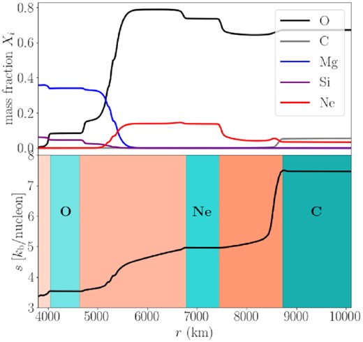
Initial chemical composition (top) and entropy profile (bottom) for the shell burning simulation. The model covers the region from |$3800$| to |$31\,200\, \mathrm{km}$| in radius, or |$1.88$| to |$5.03\, \, {\rm M}_{\odot }$| in mass coordinate. There are three distinct convective burning regions (turquoise) that persist throughout the course of the simulation. From left to right, these are the oxygen (1.95–2.10 |$\, {\rm M}_{\odot }$|), neon (2.47–2.55 |$\, {\rm M}_{\odot }$|), and carbon (2.71–5.03 |$\, {\rm M}_{\odot }$|) burning shell, respectively. Convectively stable zones (orange) correspond to regions with positive entropy gradients.
The extent and location of the convective and stable regions change somewhat over the course of the simulation because of the contraction of the shells, variations in burning rate, and convective entrainment. The evolution becomes very dynamical in the last minutes prior to collapse with considerable modifications to the structure. Convection is fully developed by |$100\, \mathrm{s}$| (corresponding to about three convective turnover times for the oxygen shell), after which time the inner convective region expands, then after |$300\, \mathrm{s}$| moves inwards again, staying roughly constant in radial extent for several minutes. By |$600\, \mathrm{s}$| the inner convectively stable region has disappeared completely, and the inner convective region covers around |$1000\, \mathrm{km}$|, effectively doubling its width and growing by a factor three in mass by the time of core collapse due to a dramatic acceleration of entrainment right before collapse. Between about |$300$| and |$500 \, \mathrm{s}$|, we have stable, quasi-stationary convection that is affected neither by initial transients, nor by the accelerating contraction right before collapse. Our analysis of differential rotation therefore mostly focuses on this phase of the simulation.
The numerical treatment is largely the same as in Müller et al. (2016). The simulation uses an overset Yin-Yang grid (Kageyama & Sato 2004; Melson, Janka & Marek 2015) with a resolution of 450 × 56 × 148 zones in radius, latitude, and longitude on each Yin-Yang patch, corresponding to a resolution of 2° in angle. The momentum equation is reformulated according to equations (23) and (24) of Müller (2020) to improve angular momentum conservation. The 19-species nuclear reaction network of Weaver, Zimmerman & Woosley (1978) is used for nuclear burning.
4 RESULTS
4.1 Spherical Favre analysis
In Fig. 2, we show the spherically averaged specific angular momentum |$\tilde{l}_z$| and angular velocity |$\tilde{\Omega }_z$| as functions of mass coordinate m (rather than r to avoid changes in the location of convective zones for a better comparison by eye). The comparison of the initial rotation profile with rigidly rotating convection zones with profiles at |$t=114\, \mathrm{s}$| (once convection is fully developed) and |$t=542\, \mathrm{s}$| (2 min before collapse) reveals two important phenomena. The secular violation of angular momentum conservation implies that we must exercise caution in taking the emerging angular momentum distribution as a steady-state solution at face value. The differential rotation within the convective zones may still represent some form of quasi-steady state if it emerges on time scales shorter than the time-scale for numerical loss of angular momentum. With this caveat, we find that a departure from rigid rotation develops during the simulation. Interestingly, a (small) positive angular velocity gradient |$\mathrm{d}\tilde{\Omega }_z/\mathrm{d}r$| develops, and the specific angular momentum is not mixed homogeneously. In fact, the angular momentum gradient become steeper than for rigid rotation, which is diametrically opposite to the emergence of a profile with constant specific angular momentum in the 2D model of Arnett & Meakin (2010) and the 3D simulation of Yoshida et al. (2021b).
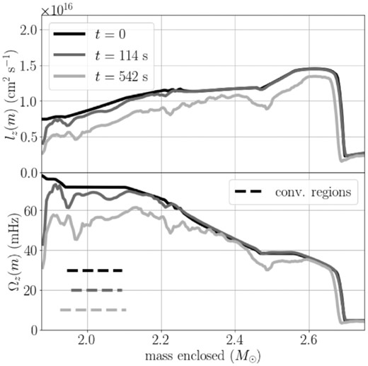
Spherically averaged (mean) specific angular momentum 〈l|$z$|〉 (top panel) and angular velocity 〈Ω|$z$|〉 (bottom panel) as a function of enclosed mass m at |$0\, \mathrm{s}$| (black), |$112\, \mathrm{s}$| (grey), and |$542\, \mathrm{s}$| (light grey). The plots completely cover the inner two convective zones around |$1.95 \rm \!-\! 2.10$| and |$2.45\rm \!-\! 2.55\, {\rm M}_{\odot }$|, which are visible as flat plateaus in Ω|$z$| at the beginning of the simulation (black curve). The radial extent of the inner (oxygen) burning shell at these three times is indicated by dashed lines. Note that during the simulations |${\sim } 16 {{\ \rm per\ cent}}$| of angular momentum is lost by numerical conservation errors, which can be inferred from the changing integral under the curves in the top panel. As the simulation progresses, a positive angular velocity gradient emerges in the inner convective shell and the angular momentum gradient steepens, indicating transport of angular momentum to larger radii.
One might be concerned that angular momentum conservation errors have contributed to the development of this positive angular velocity gradient. However, comparing the turbulent angular momentum flux from the Favre analysis to the expected angular momentum flux from MLT provides more evidence that convection does not drive the angular velocity profile towards constant Ω|$z$| (as assumed in current evolutionary models of massive stars) or constant l|$z$|.
The fluxes from equations (17) and (19) at a time of |$114\, \mathrm{s}$| are plotted in Fig. 3 as hot pink and violet curves using α = 1 and α3 = 0.1. The mere fact that such an extreme choice of α3 = 0.1 is required to obtain an MLT flux FMLT,l of the same scale as Fturb already makes it obvious that MLT does not naturally describe the turbulent flux of angular momentum in the oxygen burning shell. By and large, the MLT flux does not even have the same sign as the turbulent angular momentum flux. This situation is not unique to the snapshot shown in Fig. 3 and leads to two conclusions. First, the turbulent angular momentum flux is clearly inconsistent with the assumption that convection homogenizes the specific angular momentum and tends to increase rather than decrease the angular momentum gradient in a situation that is still relatively close to uniform rotation. Secondly, unexpectedly small flux or source terms in a turbulent flow decomposition often suggest that some form of quasi-equilibrium balance has been established. The fact that the turbulent fluxes are so small compared to the expected MLT fluxes could therefore indicate that the differential rotation in the convection zone has already adjusted to some form of quasi-equilibrium. Further evidence to support this will be discussed later in Section 4.2.
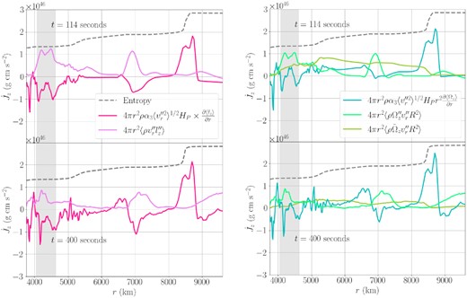
Angular momentum fluxes |$\skew{6}\dot{J}_z$| at |$t = 114\, \mathrm{s}$| after convection is fully developed but before a quasi-equilibrium state is reached (top panels), and at |$t=400\, \mathrm{s}$| during the phase of quasi-stationary convection in the grey-shaded inner convective shell (bottom panels). The structure of the star is indicated by entropy profiles (dashed), which show three convective shells at about |$4000\rm \!-\!4500$|, |$7000$|, and outside |$8500\, \mathrm{km}$|, of which only the inner shell reaches a quasi-stationary state. The left-hand panels compare the turbulent angular momentum flux from a spherical Favre composition with a base state of constant angular momentum as defined by equation (19) (light pink) to the diffusive MLT flux expected in case of adjustment to constant specific angular momentum as defined by equation (17) with α3 = 0.1 (bright pink). The right-hand panels compare the turbulent angular momentum flux (seafoam) and the meridional circulation flux (green) from equation (21) for a base state of the flow decomposition with constant Ω|$z$|, to the diffusive MLT flux expected for adjustment to uniform angular velocity with α3 = 0.05 (teal). All curves have been obtained using spatial averages over six radial zones and |$10\, \mathrm{s}$| in time. Even with these small values for α3, the MLT fluxes are qualitatively different from the actual turbulent angular momentum fluxes. In the two inner convective zones, the direction of the turbulent angular momentum flux is clearly opposite to what is required to achieve constant specific angular momentum.
It is noteworthy that the turbulent and meridional circulation terms proportional to |$\langle v_r^{\prime \prime } \Omega _z^{\prime \prime }\rangle$| and |$\langle v_r^{\prime \prime } \sin ^2 \theta \rangle \tilde{\Omega }_z$| are of comparable magnitude, though the meridional circulation term tends to be somewhat smaller inside the convection zones. The sizable contribution of the meridional circulation term indicates that large-scale turnover motions occur and influence the distribution of angular momentum. This is confirmed by further analysis.
4.2 Rotation as a function of latitude
To further elucidate the differential rotation of the inner convective shell (oxygen burning), we calculate azimuthal averages |$\bar{\Omega }_z(r,\theta)$| of the angular velocity, which are plotted in Fig. 4 (top left panel) at a time of |$400\, \mathrm{s}$|. This plot clearly demonstrates that the convective shell (which extends out to the dashed black boundary) neither conforms to the expectations of uniform rotation or uniform specific angular momentum (which would imply that Ω|$z$| is constant on cylinders and decreases with the distance from the rotation axis). Instead, the shell evolves away from the initial conditions with rigid rotation at |$\Omega _z=72\, \mathrm{mHz}$| to differential rotation that is fastest at the equator with |$\Omega _z\approx 100\, \mathrm{mHz}$|. In fact, this pattern of differential rotation already emerges after a few convective turnovers from about |$100\, \mathrm{s}$|, consistent with indications for a quasi-equilibrium state from our discussion of Fig. 3 in Section 4.1. The latitudinal variation of the angular velocity is much more pronounced than the modest radial dependence of differential rotation visible in the spherically averaged profiles in Fig. 2.
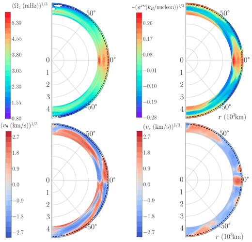
2D Favre averages over longitude φ of the angular velocity Ω|$z$| (top left), the meridional component |$v$|θ of the velocity (bottom left), the radial component |$v$|r of the velocity (bottom right), and the entropy contrast σ″′ (top right) in the inner convective region between about 4000 and |$4600\, \mathrm{km}$| at |$t= 400\, \mathrm{s}$| or 6.7 min. Note that we plot the cube root of all quantities in order to enhance the contrast at values close to zero. The outer boundary of this inner convective oxygen shell is shown as a dashed black semicircle. The convective boundary is defined as the radial coordinate at which the radial gradient of the spherically averaged entropy profile stops being negative. The angular velocity (top left) clearly shows equatorial superrotation due to the redistribution of angular momentum away from the axis of rotation. Starting from an initial configuration with solid-body rotation at |$\Omega _z= 72\, \mathrm{mHz}$| everywhere, we see a speed-up to |$\Omega _z\approx 100\, \mathrm{mHz}$| at the equator, and slowdown to |$\Omega _z \approx 60 \, \mathrm{mHz}$| at mid-latitudes, i.e. rotation at the equator is a few tens of per cent faster than at mid-latitudes. The entropy contrast σ‴ (top right) as defined by equation (24) exhibits isocontours similar to Ω|$z$|, reminiscent of the situation in the solar convection zone (Balbus 2009; Balbus et al. 2009; Balbus & Weiss 2010). The radial and meridional component of the velocity (bottom row) show a meridional circulation pattern with rising flow at the equator, sinking flow at mid-latitudes, and perhaps another circulation cell near the pole.
Fig. 4 also shows azimuthal averages of the radial and meridional velocity components |$v$|r and |$v$|θ (bottom row). These clearly reveal large-scale meridional circulation with predominant rising flow at the equator, which diverges away from the equator at larger radii, then sinks again at mid-latitudes and flows back to the equator. Another one or two circulation cells can be discerned at higher latitude, even though the third one close to the pole is less conspicuous.
4.3 Quantitative measures for differential rotation
To characterize the large-scale patterns in the differential rotation previously shown in Fig. 4, we focus on the lowest non-trivial multipoles ℓ = 2 and ℓ = 4 with equatorial symmetry and zonal wavenumber m = 0, i.e. on the coefficients Ω20/Ω00, Ω40/Ω00, l20/l00, and l40/l00. These coefficients are plotted in Fig. 5, and their values in the simulation and for the limiting cases of constant angular velocity and constant specific angular momentum are summarized in Table 1.

Normalized multipole coefficients for the specific angular momentum l|$z$| (top) and the angular velocity Ω|$z$| (bottom) for the inner convective region over time; see equations (26) and (27) for definitions. Only the lowest order even multipoles ℓ = 2 and ℓ = 4 with axisymmetry (m = 0) are shown. Initially, lℓm and Ωℓm start at values corresponding to rigid rotation (dotted lines). During the phase of quasi-stationary convection from |$300$| to |$500\, \mathrm{s}$|, the normalized quadrupole coefficients reach l20/l00 ≈ −0.77 and Ω20/Ω00 ≈ −0.45, l40/l00 ≈ 0.37 and Ω40/Ω00 ≈ 0.35 indicating superrotation at the equator (since Y20 is negative and Y40 is positive at the equator).
Lowest order even multipole coefficients of the spherical harmonics decomposition of angular momentum and angular velocity for the simulation and the limiting cases of constant angular momentum and constant angular velocity. Most of these values are included in Fig. 5.
| Rotation | Multipole | Normalized | Line type in |
|---|---|---|---|
| pattern | value | Fig. 5 | |
| (T)op/(b)ottom | |||
| Rigid | l20 | −0.45 | Dotted black (t) |
| Rigid | l40 | 0 | Dotted magenta (t) |
| Rigid | Ω20 | 0 | Dotted black (b) |
| Rigid | Ω40 | 0 | Dotted magenta (b) |
| Constant l|$z$| | l20 | 0 | Not shown |
| Constant l|$z$| | l40 | 0 | Not shown |
| Constant l|$z$| | Ω20 | 2.24 | Not shown |
| Constant l|$z$| | Ω40 | 3 | Not shown |
| Simulation | l20 | −0.77 | Solid black (t) |
| Simulation | l40 | 0.37 | Solid magenta (t) |
| Simulation | Ω20 | −0.55 | Solid black (b) |
| Simulation | Ω40 | 0.35 | Solid magenta (b) |
Once convection becomes non-linear after about |$50\, \mathrm{s}$|, the coefficients Ω20/Ω00, Ω40/Ω00, and l40/l00 start to deviate from zero, and l20/l00 takes on larger negative value compared to its initial state of l20/l00 ≈ −0.45. Consistent with the evolution away from constant specific angular momentum Ω20/Ω00 becomes negative rather than positive.
After about |$200\, \mathrm{s}$|, we see indications of a quasi-stationary state, as the normalized multipole coefficients plateau and then fluctuate around their long-term averages without any discernible secular trend for several hundred seconds. During the period between 300 and |$500\, \mathrm{s}$|, we find average values of about Ω20/Ω00 = −0.55, Ω40/Ω00 = 0.35, l20/l00 = −0.77, and l40/l00 = 0.37. Only shortly before the onset of collapse do the normalized multipole coefficients diminish. It is likely that at this stage the adjustment to a quasi-stationary state is no longer fast enough to keep pace with the contraction of the shell and its concomitant spin-up by angular momentum conservation.
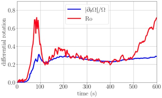
The global measure of differential rotation, |∂θΩ|/Ω as defined by equation (28) (blue curve) and the convective Rossby number in the oxygen shell (red curve) as a function of time, shown until |$600\, \mathrm{s}$|. The convective shell is in the regime of moderately fast rotation where the scaling laws of Jermyn et al. (2020a, b) predict a scaling |∂θΩ|/Ω ∼ Ro3/5. The degree of differential rotation in the oxygen shell is roughly consistent with this prediction.
For comparison, we also estimate Ro for the Yoshida et al. (2021b) simulation. Using their averaged values of the turbulent velocity and the rotational velocity in the Si/O-rich layer (|$5.5 \times 10^7$| and |$2.0 \times 10^7\, \mathrm{cm}\, \mathrm{s}^{-1}$|, respectively), we estimate their convective Rossby number to be Ro = 2.75, i.e. in the regime of ‘slow rotation’ (Ro > 1). If these global scalings are correct, and the simulation has reached a steady state, then one expects an even more extreme level of differential rotation in the latitudinal direction, compared to the simulation presented here.
5 CONCLUSIONS
We have presented a study of differential rotation in the convective oxygen burning shell of a rapidly rotating |$16\, {\rm M}_{\odot }$| helium star based on a 3D simulation with the prometheus code (Fryxell et al. 1989, 1991). Starting from a 1D stellar evolution model with rigid rotation in convection zones, we find that the convective oxygen shell naturally develops differential rotation, with the angular momentum distribution reaching a quasi-steady state after a few turnover times. Different from previous simulations in 2D (Arnett & Meakin 2010) and 3D (Yoshida et al. 2021b), the rotation profile does not tend towards uniform specific angular momentum in the convective zone. Instead the differential rotation is characterized by a positive angular velocity gradient and faster rotation at the equator by several tens of per cent.
We performed a turbulent flow decomposition based on spherical and azimuthal Favre averages to quantitatively analyse the distribution and transport of angular momentum within the computational domain. The flow decomposition shows that the turbulent transport of angular momentum is clearly not described by a 1D mixing-length theory ansatz with diffusive fluxes that drive the rotation profile towards constant angular velocity or constant specific angular momentum. Because of significant fluctuations in the spherically averaged angular momentum and angular velocity profiles, it is, however, more difficult to judge the magnitude of the radial angular velocity gradient and the significance of the deviation from uniform rotation in an effective 1D description as used in stellar evolution models. There is much stronger evidence for differential rotation with latitude. 2D flow averages reveal a global flow pattern with meridional circulation, excess angular velocity, and an entropy deficit at the equator. A quantitative analysis shows that the degree of differential rotation remains stable for several hundred seconds after an initial adjustment phase, suggesting that a quasi-equilibrium state has been reached. When the oxygen shell contracts significantly and the burning speeds up shortly before collapse, the quasi-equilibrium can no longer be maintained, and the ‘superrotation’ of the equatorial region becomes less pronounced.
The pattern of differential rotation found in our simulation is conspicuously similar to observations of the Sun (Howe 2009) and Sun-like stars (Benomar et al. 2018). Our model roughly fits recently proposed analytical scaling laws that relate the degree of differential rotation to the convective Rossby number (Jermyn et al. 2020a, b), and is consistent with compressible simulations of stellar surface convection at similar Rossby numbers of |${\sim }0.2\texttt {-}0.4$| (e.g. Käpylä et al. 2011; Mabuchi et al. 2015). This suggests that similar mechanisms may be at play as in surface convection zones. Specifically, the meridional flow pattern with superrotation and an entropy deficit at the equator may be explained as a result of thermal wind balance (Balbus et al. 2009). Due to the more dynamical nature of convective burning in our model compared to solar surface convection, a detailed analysis of angular momentum transport and force balance within the convective zone is not feasible within the current study. Longer simulations of more steady phases of late-stage burning may reveal more clearly how buoyancy, inertial forces, and turbulent stresses determine the pattern of differential rotation. Future simulations should also include magnetic fields, although these may not change the picture qualitatively based on evidence from observations and simulations (for an overview, see Jermyn et al. 2020b). It is also desirable to confirm the current results at higher resolution and minimize numerical non-conservation of angular momentum, even though we have used a formulation of the momentum equation that improves angular momentum conservation (Müller 2020). However, our analysis of turbulent fluxes and the large-scale meridional flow structure suggests that the superrotation that we observe is physical and not due to a numerical violation of angular momentum conservation.
Since our findings are clearly different from the 2D simulation of Arnett & Meakin (2010) and the recent short 3D simulation of Yoshida et al. (2021b), further investigation of late-stage convection in rotating massive stars is required. There is evidently a tension between their results and ours, as our study suggests that convection may steepen rather than flatten specific angular momentum gradients. However, there is not necessarily a contradiction. The 2D results of Arnett, Meakin & Young (2009) may well be due to the constraint of axisymmetry, which can qualitatively affect the nature of turbulent convective flow. The 3D results of Yoshida et al. (2021b) only covered few convective turnovers and may not have reached steady-state differential rotation. During an initial dynamical adjustment phase, it is conceivable that advective transport may effect some homogenization of specific angular momentum before a true steady state is reached. Such a phenomenon may play a role towards the end of our simulation as well when convection speeds up and the equatorial superrotation becomes less pronounced. Given the conspicuous similarities with simulations of stellar surface convection, we believe, however, that our longer simulation probably gives a better representation of the differential rotation that will emerge in the long run and be maintained over evolutionary time scales. An alternative explanation could be that the model of Yoshida et al. (2021b) selects an antisolar pattern of differential rotation. This might make their model conform with the scaling laws of Jermyn et al. (2020a, b), which would predict stronger differential rotation for their model, which is characterized by a higher Rossby number than ours. No firm conclusions on the reasons for the disagreement between our simulation and theirs can be drawn at this stage.
If the interior convection zones in massive stars are generically characterized by differential rotation with a positive angular velocity gradient, this could have interesting implications for the pre-collapse rotation rates and magnetic fields of supernova progenitors, and in particular for the proposed evolutionary channels for hypernovae and GRB supernovae. The cores of supernova progenitors might be spun down even more strongly than predicted by current stellar evolution models, making it more difficult to achieve the rotation rates required for the millisecond magnetar scenario, but easier to achieve sufficient angular momentum in shells a few solar masses away from the core as required for disc formation in the collapsar scenario (Woosley 1993; MacFadyen & Woosley 1999). However, this remains in the realm of speculation at this point and will need to be investigated using stellar evolution models that appropriately account for superrotation in convective zones. While it is relatively easy to relax the assumption of uniform rotation in convective zones in stellar evolution models (Heger & Müller, in preparation), capturing the nuances of the underlying physics is likely more difficult, especially when the findings from 3D models are not fully understood either. An advection–diffusion approach to angular momentum transport of Maeder & Zahn (1998) or generalizations thereof (Takahashi & Langer 2021) may be an appropriate starting point for projecting the results of 3D simulations into 1D stellar evolution models in a more consistent manner.
ACKNOWLEDGEMENTS
We thank A. Heger for fruitful discussions and for providing data for progenitor model HE16O during the pre-collapse phase, and I. Mandel for fruitful discussions. We thank our referee, R. Hirschi, for his careful reading of the earlier version, and for helpful suggestions and comments that improved our manuscript. LM acknowledges support by an Australian Government Research Training (RTP) Scholarship, and a Monash University Post Graduate Publication Award (PPA). BM has been supported, in part, by the Australian Research Council through a Future Fellowship (FT160100035). This research was undertaken with the assistance of resources obtained through the National Computational Merit Allocation Scheme and ASTAC from the National Computational Infrastructure (NCI), which is supported by the Australian Government and was supported by resources provided by the Pawsey Supercomputing Centre with funding from the Australian Government and the Government of Western Australia.
DATA AVAILABILITY
The data underlying this manuscript will be shared on reasonable request to the authors, subject to considerations of intellectual property law. Additional movies can be found here.
Footnotes
Note that the thermal wind equation is usually derived from the vorticity equation, but follows directly from equation (2) after assuming a radial pressure gradient, which makes the concept of force balance more obvious.
This can be derived by noting that |$l_z=r^2\sin ^2 \theta \Omega _z = r^2 \left(\frac{4}{3} \sqrt{\pi }Y_{00} -\frac{4}{3} \sqrt{\frac{\pi }{5}} Y_{20}\right)\Omega _z$|, so for Ω|$z$| = const. only the coefficients with ℓ = 0 or ℓ = 2 and m = 0 remain in the spherical harmonics expansion of the specific angular momentum.
For l|$z$| = const., one has Ω|$z$| = l|$z$|/(r2sin 2θ), and the ratio Ωℓm/Ω00 is determined by the values of |$Y_{\ell m}^{*}$| at the poles of the integrand in equation (27).
