


ABSTRACT
We here present the luminosity function (LF) of globular clusters (GCs) in five nearby spiral galaxies using the samples of GC candidates selected in Hubble Space Telescope mosaic images in F435W, F555W, and F814W filters. Our search, which surpasses the fractional area covered by all previous searches in these galaxies, has resulted in the detection of 158 GC candidates in M81, 1123 in M101, 226 in NGC 4258, 293 in M51, and 173 in NGC 628. The LFs constructed from this data set, after correcting for relatively small contamination from reddened young clusters, are lognormal in nature, which was hitherto established only for the Milky Way (MW) and Andromeda among spiral galaxies. The magnitude at the turn-over (TO) corresponds to MV0(TO) = −7.41 ± 0.14 in four of the galaxies with Hubble types Sc or earlier, in excellent agreement with MV(TO) = −7.40 ± 0.10 for the MW. The TO magnitude is equivalent to a mass of ∼3 × 10⁵ M⊙ for an old, metal-poor population. MV0(TO) is fainter by ∼1.16 magnitude for the fifth galaxy, M 101, which is of Hubble type Scd. The TO dependence on Hubble type implies that the GCs in early-type spirals are classical GCs, which have a universal TO, whereas the GC population in late-type galaxies is dominated by old disc clusters, which are in general less massive. The radial density distribution of GCs in our sample galaxies follows the Sérsic function with exponential power-law indices, and effective radii of 4.0–9.5 kpc. GCs in the sample galaxies have a mean specific frequency of 1.10 ± 0.24, after correcting for magnitude and radial incompleteness factors.
1 INTRODUCTION
Globular clusters (GCs) are among the oldest objects in the Universe. Their relatively high luminosities (MV = −5 to −10) and compact sizes (half-light radius of a few parsecs) allow them to be readily detectable in nearby external galaxies (Harris 1996). Their low metallicities (log [Fe/H] ≲ −0.5) and enhancements of α elements (log [O/Fe] ≥ 0.20) suggest that they are formed at very early epochs of galaxy formation (Binney & Merrifield 1998). The GC formation requires highly efficient star formation, usually associated with intense starburst activity (Bastian 2008). Star formation in the spheroids (early-type galaxies, spiral bulges, and haloes) represents one such activity in the early Universe. Interactions and mergers between galaxies provided the next epochs of star formation efficient enough to form massive star clusters such as GCs (Whitmore & Schweizer 1995). These intermediate-age clusters are similar in size and mass as the young massive clusters, also known as Super Star Clusters (SSCs), seen in presently active starburst regions (O’Connell et al. 1995). In this work, we refer to as SSCs all those relatively younger clusters associated to discs of galaxies and reserve the word GCs to describe old clusters associated to spheroids. Because of their early formation, the properties of GC systems in galaxies provide important constraints on models of galaxy formation and evolution (Ashman & Zepf 1998).
A variety of GC system properties that are potentially relevant to cosmological theories of galaxy formation have been identified. These include, colour distribution (Larsen et al. 2001; West et al. 2004), luminosity function (Reed, Harris & Harris 1994; Whitmore et al. 1995), radial density distribution (Bassino, Richtler & Dirsch 2006; Kartha et al. 2014), specific frequency as a function of galaxy type (Harris & van den Bergh 1981; Peng et al. 2008), total number of GCs as a function of supermassive black hole masses (Burkert & Tremaine 2010; Harris & Harris 2011; Harris et al. 2014), and the nature of their size distribution (Kundu & Whitmore 1998; Larsen et al. 2001; Webb, Harris & Sills 2012). These properties have been exhaustively reviewed in Brodie & Strader (2006).
Elliptical galaxies have been the most commonly used targets for the study of GC systems. This is principally because of the relative ease with which GCs can be identified when superposed on a smooth light distribution in these galaxies, as compared to the inhomogeneities inherent to the discs of galaxies. In addition, the identification procedure of GCs in disc galaxies has to take into account possible contamination from reddened young SSCs and intermediate-old (age∼1–10 Gyr) SSCs. Correction of GC magnitudes and colours for the effects of dust in the interstellar medium also becomes more important in spiral galaxies, than in elliptical galaxies.
The most important characteristic of GC systems is the existence of bimodality in their colour distribution (Zepf & Ashman 1993; Gebhardt & Kissler-Patig 1999; Larsen et al. 2001). This bimodality is understood to be due to an underlying bimodal distribution of GC metallicities (Brodie & Strader 2006). Elliptical galaxies with well-determined metallicities confirm the existence of such a bimodal distribution in metallicities (e.g. Cohen, Blakeslee & Ryzhov 1998; Usher et al. 2012). This has led to the division of GC systems into two sub-populations: red and blue, corresponding to metal-rich and metal-poor populations, respectively. These two sub-populations show differences in other properties, such as size and spatial distribution (Kundu & Whitmore 1998; Larsen & Brodie 2000a; Webb et al. 2012), suggesting possibly two independent formation channels of GC systems.
The GC luminosity function (GCLF) is another property that is well established in elliptical galaxies. GCLFs are described by lognormal distributions with M0, V = −7.40 ± 0.25 and σ = 1.40 ± 0.06 (e.g. Reed et al. 1994; Whitmore et al. 1995). The GCLF is often suggested to be a universal function (e.g. Hanes 1977b; Richtler 2003) in elliptical galaxies, and have been used as a standard candle for the determination of distances to their host galaxies (e.g. Richtler 2003). Among spiral galaxies, the lognormal nature of LFs have been firmly established only in the Milky Way (e.g. Harris 1996; Bica et al. 2006) and Andromeda (e.g. Peacock et al. 2010), the only two spiral galaxies where GC system properties have been reasonably well-characterized, with values of M0, V = −7.33, σ = 1.23 (Secker 1992; Reed et al. 1994) and M0, V = −7.6 ± 0.15, σ = 0.82 (Secker 1992; Reed et al. 1994), respectively. Within the errors of measurements, these values are in agreement with the TO found in elliptical galaxies (Ashman, Bird & Zepf 1994). Using the catalogue of Harris (1996) with 143 GCs, Jordán et al. (2007) found M0, V = −7.40 ± 0.10, σ = 1.15 ± 0.10 for MW. Fall & Zhang (2001) reproduced the lognormal form, as well as the TO value of the Galactic GCs by evolving dynamically clusters obeying power-law mass functions under the gravitational potential of the Milky Way. The uniformity in the TO values in spite of GC systems being constituted of two independently formed sub-populations puts strong constraints on the formation scenarios of metal-rich and metal-poor sub-populations.
The total number of GCs in galaxies (NGC) is another property that strongly constraints the formation scenarios of galaxies. Hanes (1977a) found that NGC is proportional to the mass of its host galaxy and is independent of its morphology. Harris & van den Bergh (1981) defined the specific frequency, SN, defined as the number of GCs per absolute magnitude in the V-band, normalized to MV = −15 mag: SN|$= {N}_{\text{G}\text{C}}\times 10^{0.4({M}_{V}+15)}$|. They found that SN of a galaxy is approximately proportional to the total luminosity of the spheroidal component in the galaxy. Recent studies have shown that elliptical galaxies have a higher SN as compared to that in spiral galaxies (e.g. Peng et al. 2008; Georgiev et al. 2010).
Classical models of formation of elliptical galaxies either by merging of disc galaxies or by the multiphase dissipational collapse have serious short comings to explain all the above-discussed properties of GC systems. For example, the scenario of the formation of ellipticals by mergers of spiral galaxies predicts similar SN values in ellipticals as compared to spirals. These models require the metal-poor population forming earlier than the metal-rich clusters. On the other hand, under the hierarchical scenario of galaxy formation, metal-rich GC systems formed in-situ in the parent galaxy, which are defined as the highest peaks in density fluctuations, whereas the metal-poor GC systems formed in low-mass haloes and got accreted into host galaxy (Côté, Marzke & West 1998). The predictions from these latter models depend critically on the assumed GC system properties in spiral and dwarf galaxies, which are yet to be well established beyond the Milky Way and Andromeda.
For firmly establishing GC system properties in spiral galaxies, the GC sample should cover a substantial area of the galaxy, reaching limiting magnitudes fainter than the expected TO magnitudes. In addition, it is desirable to have observations in one of the filters blueward of the Balmer jump (∼3650 Å) at least in some fields in order to estimate the contamination of the GC sample by reddened SSCs. The first criterion requires analysis of multiple pointing Hubble Space Telescope (HST) images or ground based images taken with wide-field cameras, whereas the second one requires images deep enough to register V ∼23 mag at distances less than 10 Mpc. The third criterion requires the availability of images in the U-band covering at least for some part of the target galaxies.
The existing works on spiral galaxies do not fulfil all the above three criteria. For example, Chandar, Whitmore & Lee (2004) carried out a study of GCs in five spiral galaxies and Goudfrooij et al. (2003) of seven edge-on disc galaxies, both using HST/WFPC2 fields, but covered relatively small areas in each galaxy. Study by Young, Dowell & Rhode (2012) of two edge-on spirals covered spatially their entire optical extents, but had a limiting magnitude slightly brighter than the expected TO. Other works on spiral galaxies include Santiago-Cortés et al. (2010) and Nantais et al. (2010b) (M81; Sab), Hwang & Lee (2008) (M51; Sbc), Barmby et al. (2006); Simanton et al. (2015) (M101; Scd), Cantiello et al. (2018) (NGC 253; Sc), and González-Lópezlira et al. (2017) (NGC 4258 Sbc). None of these works fulfilled all the three criteria.
At present, multipointing HST data covering a good fraction of the galaxy angular size (see Fig. 1) and observed in multiple filters exist for a number of nearby spiral galaxies. Some of these galaxies are also observed in the F336W filter. A careful analysis of these images would be able to provide catalogues of GCs that are free from contaminating stellar and non-stellar objects, and with a good spatial coverage. In this paper, we analyse five giant spiral galaxies that fulfill all the criteria mentioned above, and are nearer than 10 Mpc.
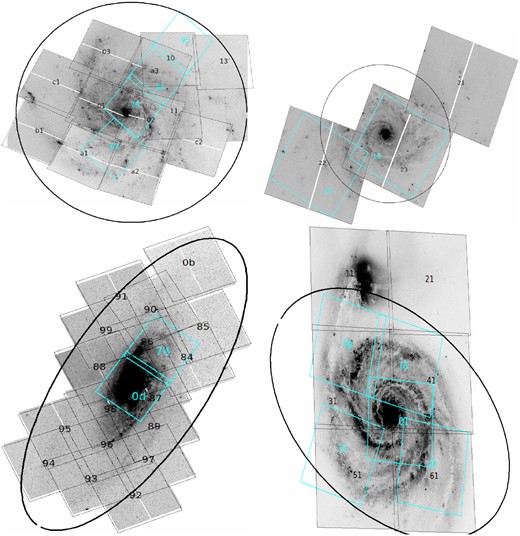
Sample of study. Galaxies are shown in F435W filter, with observation footprints superimposed. Cyan-coloured rectangles show the F336W filter footprints. The number in each footprint indicates the visit number within proposal. All galaxies are aligned such that north is up and east to the left. Black ellipse represent R25 for NGC 4258 and M51, and 0.5R25 for M101 and NGC 628. See fig. 1 in Santiago-Cortés et al. (2010) for visualization of footprints in M81.
In Section 2, we describe the sample of galaxies and the data used. In Section 3, we explain the detection and our criteria for selecting sample of GCs in the selected galaxies. Results of the completeness tests are presented in Section 4. Analysis and discussion of the properties of our GC samples is presented in Section 5. In Section 6, we give concluding remarks.
2 SAMPLE OF SPIRAL GALAXIES AND DATA
With the aim of comparing the properties of GC populations in spiral galaxies with those in elliptical galaxies, we searched for nearby giant spiral galaxies with multiple pointing HST Advanced Camera for Surveys (ACS) images in at least three optical broad-band filters. Galactic GCs typically have half-light radius rh ≲ 10 pc (Harris 1996). At the spatial resolution of ∼0.1 arcsec (image scale = 0.05 arcsec pixel−1) offered by the ACS, majority of the GCs are more extended than the Point Spread Function (PSF) up to ∼10 Mpc distances. Beyond this distance, GC selection would be heavily affected by incompleteness. Keeping this in mind, we looked for HST images of giant spiral galaxies at distances <10 Mpc. We analysed such data for five galaxies. In Table 1, we list these galaxies along with their basic properties and source of images. All these galaxies have multiple pointing HST/ACS images in F435W (B), F555W (V), and F814W (I) bands, covering a good fraction of their optical extent. In addition, all have at least one pointing in the F336W (U) filter, which allows an estimation of the contamination of our GC catalogues by reddened SSCs.
Sample of spiral galaxies.
| Name | Hubble | RA | DEC | AV | R25 | amax | d | m − M | Distance | Source | |$M_{V_{0}}$| | (B − V)0 | Scale | Source | Proposal | Number |
|---|---|---|---|---|---|---|---|---|---|---|---|---|---|---|---|---|
| Type | (J2000) | (J2000) | (mag) | (′) | (′) | (Mpc) | (mag) | method | (pc) | SSCs | ID | of fields | ||||
| (1) | (2) | (3) | (4) | (5) | (6) | (7) | (8) | (9) | (10) | (11) | (12) | (13) | (14) | (15) | (16) | (17) |
| M81 | Sab | 09:55:33.1 | 69:03:55 | 0.220 | 13.45 | 7.74 | 3.61 | 27.79 ± 0.06 | Cepheids | 1 | −21.10 | 0.91 | 0.87 | 1,2 | 11570 | 29 |
| M101 | Scd | 14:03:12.5 | 54:20:56 | 0.023 | 14.42 | 7.49 | 6.95 | 29.21 ± 0.06 | Cepheids | 2 | −21.37 | 0.44 | 1.68 | 4,6,7 | 9490,9492 | 12 |
| NGC 4258 | Sbc | 12:18:57.5 | 47:18:14 | 0.045 | 9.31 | 8.60 | 7.576 | 29.397 ± 0.032 | MASER | 3 | −21.03 | 0.67 | 1.84 | 3 | 1157 | 17 |
| M51 | Sbc | 13:29:56.2 | 47:13:50 | 0.095 | 5.61 | 3.40 | 8.43 | 29.67 ± 0.02 | SNII | 4 | −21.40 | 0.57 | 2.04 | 4,5 | 10452 | 6(4) |
| NGC 628 | Sc | 01:36:41.7 | 15:47:01 | 0.192 | 5.23 | 5.1 | 9.77 | 29.95 ± 0.04 | SNII | 5 | −20.75 | 0.50 | 2.36 | 4,8 | 10402 | 3 |
Note. (1) Galaxy Name, (2) Hubble morphological type from RC3 (Corwin, Buta & de Vaucouleurs 1994), (3,4) Right ascension, Declination, in J2000, (5): Galactic extinction from Schlafly & Finkbeiner (2011), (6) R25 from RC3 (Corwin et al. 1994), (7) amax is the angular size along the semi-major axis covered by observations, (8) Distance used in this work, (9) Distance modulus, (10) Distance estimation method, (11) Source of distances: 1. Tully et al. (2013); 2. Riess et al. (2016). 3. Reid, Pesce & Riess (2019); 4. Rodríguez, Clocchiatti & Hamuy (2014); 5. Olivares E. et al. (2010), (12,13) Absolute magnitude in V band and (B − V)0 colour from RC3 (Corwin et al. 1994), (14) HST/ACS pixel scale in pc pixel−1, (15) References to previous studies of stellar clusters: 1. Santiago-Cortés, Mayya & Rosa-González (2010); 2. Nantais et al. (2010a); 3. González-Lópezlira et al. (2017); 4. Whitmore et al. (2014); 5. Hwang & Lee (2008); 6. Barmby et al. (2006); 7. Simanton, Chandar & Whitmore (2015); 8. Adamo et al. (2017), (16) HST proposal number, (17) Number of ACS fields of each galaxy used in this work.
The Hubble Legacy Archive1 (HLA) provides images and photometric catalogues obtained with daophot2 (Stetson 1987) and SExtractor3 (Bertin & Arnouts 1996). These catalogues have been used by Whitmore et al. (2014) to study the luminosity function of star clusters in selected fields for a sample of 20 spiral and irregular galaxies. As a first step, we used these catalogues to select a sample of GCs. However, we noticed that the adjacent images had vastly different limiting magnitudes in some galaxies. A visual inspection of catalogued sources on the images suggested that the background values used in some images were inappropriate (see Appendix A). Since we are looking for a complete sample of GCs up to a given limiting magnitude, we decided to make our own catalogues on the downloaded images.
In Fig. 1, we show the images of galaxies in F435W band, with footprints superposed. In Tables 2 and 3, we give logs of observations for four of our galaxies in the optical and F336W filters, respectively. Different columns tabulate pointing IDs, exposure times, zeropoints4 (c0) in each filter. We also give the number of stars used for astrometry and RMS error in the coordinates. The fifth galaxy, M81, has been the subject of study previously by our group (Santiago-Cortés et al. 2010), and hence we directly use the GC catalog from that study.
Log of HST/ACS optical observations of our sample galaxies†.
| F435W | F555W | F814W | Astrometric | |||||
|---|---|---|---|---|---|---|---|---|
| ID | Texp | c0 | Texp | c0 | Texp | c0 | Nstars | RMS |
| (s) | (s) | (s) | ( arcsec) | |||||
| M101 | ||||||||
| 01 | 900 | 25.792 | 720 | 25.736 | 720 | 25.531 | 93 | 0.0259 |
| 02 | 900 | 25.792 | 720 | 25.736 | 720 | 25.531 | 55 | 0.163 |
| 03 | 900 | 25.792 | 720 | 25.736 | 720 | 25.531 | 38 | 0.0385 |
| a1 | 900 | 25.792 | 720 | 25.736 | 720 | 25.531 | 41 | 0.0319 |
| a2 | 900 | 25.792 | 720 | 25.736 | 720 | 25.531 | 37 | 0.278 |
| a3 | 900 | 25.792 | 720 | 25.736 | 720 | 25.531 | 11 | 0.0766 |
| b1 | 900 | 25.792 | 720 | 25.736 | 720 | 25.531 | 10 | 0.187 |
| c1 | 900 | 25.792 | 720 | 25.736 | 720 | 25.531 | 18 | 0.0925 |
| c2 | 900 | 25.792 | 720 | 25.736 | 720 | 25.531 | 21 | 0.0175 |
| 10 | 1080 | 25.792 | 1080 | 25.736 | 1080 | 25.531 | 13 | 0.0988 |
| 11 | 1080 | 25.792 | 1080 | 25.736 | 1080 | 25.531 | 29 | 0.0456 |
| 13 | 1080 | 25.792 | 1080 | 25.736 | 1080 | 25.531 | 11 | 0.0862 |
| NGC 4258 | ||||||||
| 0b | 360 | 25.767 | 975 | 25.717 | 375 | 25.520 | 6 | 0.0134 |
| 84 | 360 | 25.767 | 975 | 25.717 | 375 | 25.520 | 8 | 0.0264 |
| 85 | 360 | 25.767 | 975 | 25.717 | 375 | 25.520 | 6 | 0.0058 |
| 86 | 360 | 25.767 | 975 | 25.717 | 375 | 25.520 | 27 | 0.0049 |
| 87 | 360 | 25.767 | 975 | 25.717 | 375 | 25.520 | 35 | 0.0049 |
| 88 | 360 | 25.767 | 975 | 25.717 | 375 | 25.520 | 26 | 0.0051 |
| 89 | 360 | 25.768 | 975 | 25.717 | 375 | 25.521 | 12 | 0.0023 |
| 90 | 360 | 25.767 | 975 | 25.717 | 375 | 25.520 | 13 | 0.0090 |
| 91 | 360 | 25.767 | 975 | 25.717 | 375 | 25.520 | 5 | 0.039 |
| 92 | 360 | 25.768 | 975 | 25.717 | 375 | 25.521 | 8 | 0.025 |
| 93 | 360 | 25.768 | 975 | 25.717 | 375 | 25.521 | 9 | 0.0273 |
| 94 | 360 | 25.768 | 975 | 25.717 | 375 | 25.521 | 9 | 0.03 |
| 95 | 360 | 25.768 | 975 | 25.717 | 375 | 25.521 | 8 | 0.0145 |
| 96 | 360 | 25.768 | 975 | 25.717 | 375 | 25.521 | 20 | 0.0157 |
| 97 | 360 | 25.768 | 975 | 25.717 | 375 | 25.521 | 8 | 0.0054 |
| 98 | 360 | 25.768 | 975 | 25.717 | 375 | 25.521 | 30 | 0.0054 |
| 99 | 360 | 25.767 | 975 | 25.717 | 375 | 25.520 | 14 | 0.0128 |
| M51 | ||||||||
| 1-6 | 680 × 4 | 25.888 | 340 × 4 | 25.715 | 340 × 4 | 25.471 | 299 | 0.0482 |
| NGC 628 | ||||||||
| 21 | 1200 | 25.789 | 1000 | 25.732 | 900 | 25.528 | 9 | 0.0445 |
| 22 | 800 | 25.788 | 360 | 25.731 | 720 | 25.528 | 15 | 0.047 |
| 23 | 1358 | 25.789 | 858 | 25.732 | 922 | 25.528 | 15 | 0.034 |
Note. † Table 1 of Santiago-Cortés et al. (2010) contains observational log for 29 pointing in M81, the fifth galaxy of our sample.
Log of HST/WFC3 F336W-band observations of our sample galaxies.
| ID | Texp | c0 | Nstars | RMS | Proposal |
|---|---|---|---|---|---|
| (s) | ( arcsec) | ID | |||
| (1) | (2) | (3) | (4) | (5) | (6) |
| M101 | |||||
| 64 | 2361 | 23.546 | – | – | 13364 |
| 79 | 2382 | 23.546 | – | – | 13364 |
| 94 | 2382 | 23.546 | – | – | 13364 |
| 95 | 2382 | 23.546 | – | – | 13364 |
| NGC 4258 | |||||
| 0d | 1062 | 23.546 | 33 | 0.0154 | 13364 |
| 74 | 1062 | 23.546 | 15 | 0.0109 | 13364 |
| M51 | |||||
| 01 | 4360 | 23.546 | 163 | 0.0352 | 13340 |
| 0g | 2376 | 23.546 | 55 | 0.0191 | 13364 |
| 0i | 2361 | 23.546 | 42 | 0.0317 | 13364 |
| 76 | 2376 | 23.546 | 64 | 0.0281 | 13364 |
| 31 | 780 | 23.546 | 31 | 0.0350 | 14149 |
| NGC 628 | |||||
| 19 | 2361 | 23.546 | 15 | 0.0031 | 13364 |
| 20 | 1119 | 23.546 | 10 | 0.0321 | 13364 |
3 SOURCE DETECTION AND CLUSTER SELECTION
We used images in F814W band for detecting sources using SExtarctor. The critical detection parameters used are: detect_minarea = 5 pixel, detect_thresh = 1.4, back_size = 32 pixel and back_filtersize = 3 pixel, where each pixel corresponds to 0.05 arcsec. Using these criteria, typically we obtained several tens of thousands sources in each frame. Elaborate filtering criteria need to be implemented to select GCs from this catalogue.
As discussed in the introduction, making a catalogue of GCs is more challenging in spiral galaxies as compared to elliptical galaxies. This is because, unlike elliptical galaxies, spiral galaxies show a lot of structures at the scale comparable to the size of GCs. These structures lead to a lot of spurious sources in the SExtarctor catalogue. Filtering based on structural parameters (e.g. Mayya et al. 2008), colour (e.g. Fedotov et al. 2011), concentration index (e.g. Whitmore et al. 2014), colour–colour diagrams (e.g. Muñoz et al. 2014; González-Lópezlira et al. 2017) or a combination of these, are the most commonly used methods. In this paper, we used the cluster selection method used in Mayya et al. (2008) and Santiago-Cortés et al. (2010), which consists of using SExtractor-derived structural parameters (fwhm, area, ellipticity) to define a cluster sample, and photometric parameters (colour) to separate young clusters from GCs. The method is described in detail in Sections 3.2 and 3.4, below.
3.1 Astrometric correction of HST images
Before running SExtratctor it was necessary to astrometrize all HLA images. We performed this with the help of GAIA stars using Gaia Data Release 2 (Gaia DR2; Gaia Collaboration 2016, 2018). We used the iraf task ccmap with a second-order polynomial in coordinates to achieve this. Minimum of 10 stars were used in each pointing (5 stars in one pointing of NGC 4258), resulting in mean rms astrometric accuracies of ∼0.095 arcsec (M101), ∼0.014 arcsec (NGC 4258), ∼0.048 arcsec (M51), and ∼0.042 arcsec (NGC 628). We took into account these rms errors to identify and eliminate duplicate sources in the overlap zones between two adjacent frames. In Fig. 2, we zoom in on an image section in M101 to illustrate a typical field before and after astrometric correction. The left-hand image shows the HST coordinate system for this field, whereas the image on the right shows the corrected coordinate system. The circles show the coordinates of GAIA (Gaia DR2) stars in this field of view.
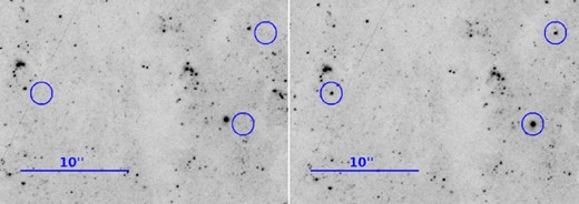
Illustration of astrometry on the HST image using a section of M101. Left-hand panel: astrometric coordinates on the downloaded image from HLA. Right-hand panel: image after applying our astrometric corrections based on the GAIA DR2 coordinates of the field stars. Three field stars in the displayed FOV are identified with blue circles of 1 arcsec radius. North is up and east to the left in these images.
3.2 Selection criteria for defining a cluster sample
In this work, we aim to obtain a sample of GCs with properties similar to those in the Milky Way, which are marginally resolved on the HST/ACS images at the distances of sample galaxies. We considered all objects with fwhm>2.4 pixel as GC candidates. This cut-off corresponds to 2.1 pc and 5.7 pc, in the nearest (M81) and farthest (NGC 628) galaxies of the sample. Thus, farther a galaxy is, lesser would be the number of compact objects we would detect. GCs do not show a mass–radius (or equivalently luminosity–radius) relationship (Gieles et al. 2010) and hence this bias is not expected to affect the LF of GCs. GCs are roundish objects, and hence their ellipticity parameter is expected to be close to zero. SExtractor-measured ellipticity even for roundish objects could be as high as 0.3, as it is measured at the isophote corresponding to the detection threshold on the background subtracted image. Another parameter that SExtractor calculates is area, with is the number of pixels enclosed by the isophote where ellipticity is measured. Both the ellipticity and area depend on the threshold used for the detection, and hence a cluster of same magnitude and fwhm can have different values of ellipticity and area, depending on the underlying background.
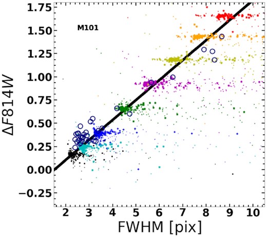
We have carried out Monte Carlo simulations to understand the behaviour of these parameters for clusters of different fwhm and magnitudes, appropriate to the background and crowding encountered in each galaxy in the F814W band. In Section 4, we describe in detail these simulations. In Fig. 3 (right-hand panel), we show the simulated clusters in area versus fwhm diagram for each of our sample galaxies. Simulations were carried out for a range of magnitudes between 19 and 24 magnitudes, for fixed values of fwhm. As expected, brighter clusters have larger areas at a given fwhm, and the area increases quadratically with fwhm for a cluster of given magnitude. We show the dependence of area with fwhm for objects of 23 mag by the blue solid curve, which is defined by the same equation, AREA = 52.5 − 1.0 FWHM + 0.50 FWHM2, for all our sample galaxies. On the left-hand panel, we show all the detected sources in fwhm versus area diagram for our five sample galaxies. The parabola defined by the simulations is shown, which separates the bonafide cluster candidates (that are above the parabola) from contaminating sources (image blemishes, stellar asterisms, image borders etc.), which dominate the number of detected sources at every fwhm. A hard cut in magnitude or area can also eliminate the contaminating objects, but the use of parabola is the most effective way to eliminate these contaminating sources, without missing many genuine clusters. GCs at the distance of sample galaxies are expected to have fwhm close to the observational lower limit of 2.4 pixels. In the top panel of Fig. 4, we show the observed distribution of fwhm for our final GC sample for one of our sample galaxies (M101), which indeed peaks at the first bin. However, we include objects up to fwhm = 10 pixels to account for possible errors in the measurement of fwhm at detection limits. Simulations suggest that even the brightest clusters (F814W = 19) do not occupy an area>500 pixels as long as the fwhm∼5 pixels, and hence we eliminated sources with area>500 pixel.

Left-hand panel: Selected GCs (red dots) compared to all SExtractor sources (black dots) in area versus fwhm plane for our 5 sample galaxies. GCs have (B − I)0 > 1.5 mag, 2.4<fwhm/pix<10 and are above the parabola (blue line). Clusters bluer than this limit are SSCs which are identified by blue dots. Black dots above the parabola are extended sources with ellipticities>0.3, and hence do not satisfy all cluster selection criteria. Right-hand panel: area versus fwhm for simulated star clusters. The fwhm of mock clusters are fixed at 2.0 (black), 2.4 (cyan), 3.0 (blue), 4.0 (green), 5.0 (magenta), 6.0 (yellow), 7.0 (orange), and 8.0 (red) pixels. For each fixed fwhm, 100 mock clusters between 19 and 24 magnitudes are generated, which are shown by symbols of different sizes (successively smaller sizes for fainter sources; see the bottom-most right-hand panel for a guide on the symbol size). Most of the clusters with mag >23 lie below the parabola defining the minimum area–fwhm relation, and hence are rejected by our selection criteria.
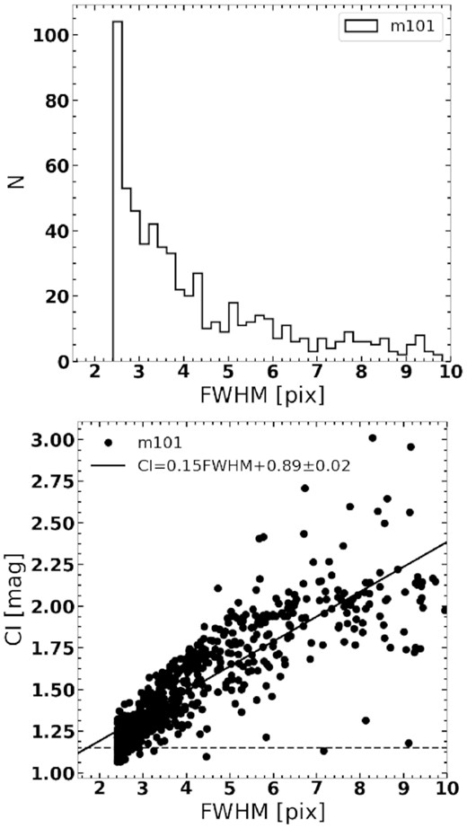
(Top) Distribution of fwhm for the candidate GCs in one of our galaxies (M101). (Bottom) Comparison of the two commonly used discriminators between clusters and stars, CI versus fwhm. Data are consistent with a linear fit (solid line whose equation is given in the top left-hand corner) above the dividing line between clusters and stars (horizontal dashed line at CI = 1.15). Data correspond to M101, which has 45 GCs below the defining line (see the text for details).
The HLA catalogues include a parameter known as concentration index (CI), defined as the difference between magnitudes measured in 1 and 3 pixel radius apertures. Some studies have made use of this parameter to discriminate between point and extended sources (e.g. Whitmore et al. 2014; Simanton et al. 2015) CI <1.15 for stars. In our study, we have used the fwhm = 2.4 pixel (0.12 arcsec), a direct discriminator between unresolved (stars) and resolved (extended) sources. In the bottom panel of Fig. 4, we show CI against the fwhm for all our clusters for M101. As expected, the two parameters are correlated. The minimum CI (1.07) for our sample clusters is slightly less than 1.15, the value adopted in other studies. Forty-five (∼4 per cent) of our sources would not have been classified as stellar cluster if we had adopted the CI criterion. A visual inspection of these borderline objects suggests they are likely to be clusters, rather than stars. We identify these borderline cases (1.07<CI<1.15) by red dots surrounded by black circles in Fig. 8. In NGC 4258, these include two of the brightest GCs.
3.3 Aperture photometry
3.3.1 Magnitudes, colours, and aperture correction
SExtractor was also used for obtaining photometry in the three bands for all the detected sources. The photometry was carried out in 10 apertures with radii between 1 and 15 pixel (0.05 arcsec to 0.75 arcsec), using the zeropoints (c0) tabulated in Table 2 for each frame. Unlike stars, aperture correction for clusters depend on the cluster size, which is parametrized by the fwhm in SExtractor. The aperture correction is defined as the difference between magnitude at 3 pixel (0.15 arcsec) radius and the magnitude at an infinite aperture (ΔF814W = mF814W(3 pix)−mF814W(tot)). Even the most extended clusters (objects with Gaussian fwhm = 9 pixel) contain more than 98 per cent of their total flux within an aperture of 15 pixel radius, because of which we have used the magnitude in an aperture of 15 pixel radius as mF814W(tot).
We used the results of our experiments with simulated clusters, described later in Section 4, to obtain the correction as a function of measured fwhm in each galaxy. The results are shown in Fig. 5 for M101. A group of horizontally distributed points corresponds to the same input fwhm. The measured fwhm for fainter clusters tends to be systematically larger than the input fwhm, which is the reason for the horizontal spread. The aperture corrections (open circles) obtained for 35 isolated clusters with good photometry (error <0.005 mag in 9 pixel) is also shown in the figure. Both the simulated and observed corrections smoothly increase with the fwhm. For the simulated data, we obtained mean values of measured fwhm and correction for each input fwhm and fitted these mean values by a straight line which is shown by the solid line. The fitted results (the slope m, and the abscissa, b) for all the sample galaxies are given in Table 4.
Apertures corrections versus FWHM for observed (open circles) and simulated (coloured points) star clusters in M101. The line is the linear fit to the simulated points.
Aperture correction coefficients and typical photometric errors in (F435W − F555W)0 colour for the sample galaxies.
| Galaxia | m | b | σBV |
|---|---|---|---|
| (1) | (2) | (3) | (4) |
| M81 | 0.193 ± 0.004 | −0.277 ± 0.026 | 0.10 |
| M101 | 0.215 ± 0.004 | −0.330 ± 0.025 | 0.21 |
| NGC 4258 | 0.193 ± 0.007 | −0.279 ± 0.045 | 0.10 |
| M51 | 0.218 ± 0.004 | −0.354 ± 0.024 | 0.16 |
| NGC 628 | 0.225 ± 0.003 | −0.358 ± 0.022 | 0.19 |
Note. σBV is the average standard deviation estimated in the (F435W − F555W)0 colour in bins of 0.2 mag in (F435W − F814W)0 colour for clusters with (F435W − F814W)0 > 1.5.
We applied these corrections to the F814W aperture magnitudes of 3 pixel radius of all cluster candidates to obtain their total magnitudes. Colours (F435W − F814W, F435W − F555W, and F555W − F814W), however are obtained by subtracting magnitudes in the corresponding filters at 3 pixel radius aperture. This procedure ensures that errors on colours are smaller than the aperture corrected magnitudes. The errors on colours were calculated by quadratically summing the magnitude errors in the two bands forming a colour.
3.3.2 Photometric error estimation
Formal errors5 on photometric measurements are obtained using the formula: MAGERR = 1.086 × (FLUXERR/FLUX), where |$FLUXERR=\sqrt{\displaystyle \sum _{i\in A} (\sigma _{i}^{2}+\frac{p_{i}}{g_{i}})}$|, with A representing the set of pixels defining the photometric aperture, σi, the standard deviation of noise (in ADU) estimated from the local background, pi the background-subtracted image pixel value, and gi the effective detector gain in e-/ADU at pixel i. However, small-scale variations in the disc background gives rise to additional errors while carrying out photometry of non-stellar objects such as GCs, that are usually larger than the formal errors. We use the colour–colour diagram (F435W − F555W)0 versus (F435W − F814W)0 to estimate the real errors on our colours. In Fig. 6, we illustrate the method adopted for this. In this plot, we show the colours for star clusters in NGC 4258, with the SSPs with Z = 0.001 and 0.019 metallicities from Bruzual & Charlot (2003). The reddening vector for AV = 4 mag is also shown. The reddening vector and the evolutionary trajectory are parallel in this colour–colour diagram, implying the spread in the (F435W − F555W)0 colour for a fixed (F435W − F814W)0 colour (and vice versa) is entirely due to observational errors. We calculated the dispersions in colour for each axis for fixed bins of 0.2 mag width in the other axis. In the figure, we show these dispersions by crosses places at every 0.4 mag. There is a tendency for slightly higher error for the reddest colours. We take into account this dispersion in each colour as an additional source of error while comparing observational colours with model colours.
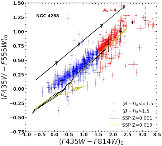
Colour–colour diagram showing all SExtractor-detected clusters for one of our sample galaxies (NGC 4258). The SSP evolution between 0 and12 Gyr at two metallicities and the reddening vector for AV = 4 mag, with arrow heads placed at 1 mag intervals, are shown. Both the evolution and the reddening move the points along the same direction, and hence the spread in either axis around a mean local value (the crosses) is entirely due to observational errors in colours.
3.4 The sample of GCs
We define GCs as old (age>10 Gyr) metal-poor (Z ≲ 0.001) clusters, having properties similar to that for the sample of Galactic GCs. However, unlike the Galactic GCs, extragalactic GCs cannot be selected by their visual appearance even on the HST images. Our cluster sample contains GCs as well as relatively young clusters, such as SSCs. In Table 5, we list the source detection statistics in each galaxy. The second column contains all SExtractor-defined sources, with the column 3 containing the number of cluster sources. Cluster samples in spiral galaxies contain more SSCs than GCs, and hence quantitative criteria are required to discriminate between GCs and SSCs. Cluster colour is the most useful discriminator for achieving this. For example, metal-poor SSPs (Z ≤ 0.001) predict B − I ≥1.5 mag for populations older than ∼3 Gyr (Bruzual & Charlot 2003).
Source detection and selection statistics.
| Galaxy | All | NSSC + GC | NGC | |$N_{\rm GC}^U/N_{\rm GC}$| | Ncont/NGC |
|---|---|---|---|---|---|
| (1) | (2) | (3) | (4) | (5) | (6) |
| M81 | 565438 | 433 | 158 | 0.65 | 0.20 |
| M101 | 1215533 | 3091 | 1123 | 0.14 | 0.32 |
| NGC 4258 | 1360607 | 626 | 226 | 0.35 | 0.35 |
| M51 | 452747 | 1196 | 293 | 0.52 | 0.25 |
| NGC 628 | 224108 | 608 | 173 | 0.41 | 0.14 |
Note. (1) Galaxy. (2) All sources (stellar+non-stellar+spurious) detected by SExtractor in all the pointings over the target galaxy. (3) Those sources satisfying the criteria explained in Section 3.2 to be identified as a cluster. (4) Subset of red (B − I >1.5 mag) sources in column 3. (5) Fraction of total number CGs with photometry in an ultraviolet filter. (6) Fraction of contaminants (reddened SSCs) in our GC sample.
In Fig. 7, we plot the distribution of (F435W − F814W)0 colours for all clusters (black histogram) and for clusters brighter than MF814W = −9 mag (red histogram) in each galaxy. The latter is multiplied by a factor which is indicated in the figure annotation. For the bright cluster sample, four of the five galaxies studied here show a bimodality in the distribution, the exception being M101. The colour that separates the two distributions is nearly the same in all these galaxies, and corresponds to the (F435W − F814W)0 = 1.5 mag bin. The full cluster sample also shows a minimum in the distribution close to this colour in four of the galaxies. In M101, although the evidence for bimodality is not strong for the bright cluster sample, the total sample indicates bimodality with the saddle point again corresponding to the (F435W − F814W)0 = 1.5 mag. The blue and red distributions correspond to the SSCs, and GCs, respectively. Based on this, we use (F435W − F814W)0 = 1.5 mag to separate GCs and SSCs. Column 4 of Table 5 lists the number of clusters classified as GCs using this colour criterion. Coordinates and photometry for each of the selected GCs are given in Table 6. The table in the body of the text contains data only for three brightest objects in each galaxy. The entire table is available in electronic version.
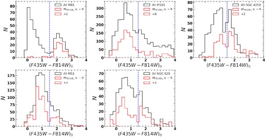
Colour histogram of all (SSC+GC) cluster candidates. The black line shows the colour distribution over the entire range of magnitudes, whereas the red histogram shows the distribution for bright (MI ≤ −9) clusters. The latter histogram values are multiplied by a factor indicated in each panel. The vertical line at (F435W − F814)0 = 1.5 separates SSCs from GCs.
Observational properties of the brightest three GCs in each sample galaxy.
| ID | RA | DEC | I | (B − I)0 | (B − V)0 | (U − B)0 | FWHM | AREA | CI | MF814W | rgc (kpc) | FLAG |
|---|---|---|---|---|---|---|---|---|---|---|---|---|
| (1) | (2) | (3) | (4) | (5) | (6) | (7) | (8) | (9) | (10) | (11) | (12) | (13) |
| M81-GC1 | 148.84125 | 69.110425 | 16.13 ± 0.03 | 2.06 ± 0.10 | 1.10 ± 0.10 | 1.63 ± 0.10 | 3.62 | – | – | −11.66 | 3.03 | 02 |
| M81-GC2 | 148.94123 | 69.050097 | 16.75 ± 0.03 | 2.24 ± 0.10 | 1.27 ± 0.10 | 2.05 ± 0.10 | 3.45 | – | – | −11.03 | 1.54 | 03 |
| M81-GC3 | 149.11440 | 69.019380 | 16.95 ± 0.03 | 1.78 ± 0.10 | 1.00 ± 0.10 | 1.43 ± 0.10 | 5.82 | – | – | −10.84 | 5.87 | 02 |
| M101-GC1 | 210.824946 | 54.318723 | 17.63 ± 0.02 | 2.51 ± 0.00 | 1.20 ± 0.17 | 1.31 ± 0.41 | 3.07 | 449 | 1.30 | −11.57 | 4.00 | 03 |
| M101-GC2 | 210.884651 | 54.414166 | 18.57 ± 0.02 | 2.74 ± 0.00 | 1.14 ± 0.17 | – | 3.38 | 394 | 1.50 | −10.63 | 9.82 | 00 |
| M101-GC3 | 210.884508 | 54.369237 | 19.10 ± 0.02 | 2.48 ± 0.00 | 1.46 ± 0.17 | – | 2.92 | 301 | 1.39 | −10.10 | 6.31 | 00 |
| NGC 4258-GC1 | 184.729270 | 47.264868 | 17.83 ± 0.00 | 1.63 ± 0.00 | 0.79 ± 0.10 | – | 2.69 | 311 | 1.16 | −11.57 | 5.25 | 00 |
| NGC 4258-GC2 | 184.865700 | 47.210389 | 17.89 ± 0.00 | 3.37 ± 0.01 | 1.13 ± 0.10 | – | 2.79 | 165 | 1.18 | −11.50 | 16.78 | 00 |
| NGC 4258-GC3 | 184.745970 | 47.301067 | 17.97 ± 0.00 | 2.15 ± 0.01 | 0.99 ± 0.10 | 0.43 ± 0.05 | 4.03 | 440 | 1.65 | −11.42 | 0.69 | 02 |
| M51-GC1 | 202.459584 | 47.174710 | 18.90 ± 0.03 | 2.05 ± 0.00 | 1.07 ± 0.10 | −0.06 ± 0.17 | 3.10 | 462 | 1.44 | −10.76 | 3.23 | 02 |
| M51-GC2 | 202.507117 | 47.241845 | 19.18 ± 0.03 | 3.50 ± 0.00 | 1.52 ± 0.10 | 1.17 ± 0.17 | 2.77 | 271 | 1.35 | −10.48 | 7.96 | 03 |
| M51-GC3 | 202.469420 | 47.253906 | 19.31 ± 0.03 | 1.75 ± 0.00 | 1.25 ± 0.10 | – | 2.47 | 281 | 1.24 | −10.35 | 8.80 | 00 |
| NCG628-GC1 | 24.221429 | 15.788914 | 18.28 ± 0.03 | 2.51 ± 0.00 | 1.08 ± 0.16 | 1.82 ± 0.07 | 3.33 | 471 | 1.56 | −11.66 | 7.84 | 03 |
| NCG628-GC2 | 24.171023 | 15.782500 | 19.13 ± 0.03 | 1.90 ± 0.00 | 0.68 ± 0.16 | 0.28 ± 0.09 | 2.75 | 243 | 1.37 | −10.81 | 0.52 | 02 |
| NCG628-GC3 | 24.212973 | 15.734987 | 19.71 ± 0.03 | 3.15 ± 0.00 | 1.25 ± 0.16 | – | 2.62 | 183 | 1.16 | −10.23 | 10.48 | 00 |
Note. (1) Assigned name, which follows the convention of GAL-GCn, where GAL stands for galaxy name and n is 1 for the brightest object in the F814W filter, and increases sequentially as the magnitude increases. (2,3) Right ascension, Declination, coordinates in J2000. (4) Magnitude in F814W-band and magnitude error from SExtractor and aperture correction, added in quadrature, (5) (F435W − F814W)0 colour, the error is the quadrature sum of the error in each band from SExtractor. (6) (F435W − F555W)0 colour, error is quadrature sum as in column 5. In the case of M81 the colour is (F435W − F606W)0. (7) (F336W − F435W)0 colour, the error is the quadrature sum of the error in each band. In the case of M81 the colour is. (u − g)0. (8) FWHM in pixel units from SExtractor. (9) AREA in pixels from SExtractor. (10) Concentration index, defined as the difference between magnitudes measured in 1 and 3 pixel radius apertures. (11) Absolute magnitude in F814W-band. (12) Galactocentric distance of the GC in kiloparsec. (13) FLAG classification: 00 clusters without U-band photometry; 01 determined as a reddened young cluster from U-band photometry; 02 – determined as bonafide GC from U-band photometry; and 03 – error in U-B is likely to be larger than the indicated formal error.
The red tail of the reddened SSC colours most likely extends beyond the colour cut of (F435W − F814W)0 = 1.5 mag, and hence colour-selected GC sample in spiral galaxies is expected to have some contamination from the reddened SSCs. The SSC population has a long tail on the red side, which is either due to a spread in reddening, or/and due to a spread in ages of SSCs. In either case, the red tail of SSC distribution has very few clusters beyond (F435W − F814W)0 >1.5 mag. The estimation of contaminating objects in the GCs samples is discussed in Section 3.5.
In Fig. 8, we plot all candidate clusters in a colour–magnitude diagram (CMD) formed using |$M_{F814W_{0}}$| versus (F435W − F814W)0, where SSCs and GCs are shown by blue and red points, respectively. The evolutionary loci of clusters for Simple Stellar Population (SSP) models from Bruzual & Charlot (2003) at typical metallicities of SSCs (Z = 0.008∼1/3 solar) and GCs (Z = 0.001) are shown. These models correspond to synthetic clusters of mass = 1 × 10⁶ |$\mathcal {M}_{\odot }$| obeying the Kroupa initial mass function (IMF) between masses 0.1 and 100 |$\mathcal {M}_{\odot }$|. If the GCs are as old as 12 Gyr, the range of magnitudes covered by the GCs corresponds to mass range shown by the dashed vertical line, and the range of colours corresponds to reddening equivalent to AV = 0 to ∼2 mag.
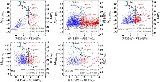
|$M_{F814W_{0}}$| versus (F435W − F814W)0 CMD of all cluster candidates in our sample of galaxies. Candidates having (F435W − F814W)0 >1.5 mag are GC candidates (red dots), and bluer objects are young disc cluster candidates (blue dots). The evolutionary locus of the SSPs from Bruzual & Charlot (2003) for two metallicities (Z = 0.001, black solid line and Z = 0.008, black dashed line), of mass = 1 × 10⁶ |$\mathcal {M}_{\odot }$| and Kroupa IMF, are shown. Locations corresponding to selected ages (0.1, 0.5, 1, 3, 6, and 12 Gyr) are marked (cyan and magenta triangles in each SSP). The chosen colour cut separates clusters older than 3 Gyr from the younger ones for unreddened SSPs. The reddening vectors with AV = 1 mag are shown for 3 cluster masses for an SSP of 12 Gyr age and Z = 0.001, typical values expected for GCs. The majority of the GC candidates are in the zone occupied by clusters of mass 1 × 10⁵ to 5 × 10⁶ |$\mathcal {M}_{\odot }$| and AV between 0 and 1 mag. Encircled red dots correspond to compact GC candidates (1.07 <CI<1.15; see section 3.2 for details) in our sample.
3.5 Contamination of the GC sample from reddened SSCs
Fig. 8 suggests that the reddened SSC colours overlap with the GC colours. The colour histogram (Fig. 7) also suggests that the distribution of the SSC colours (the bluer peak) most likely has a long tail on the redder side, that overlaps with the GC colours. Thus, contamination to some degree from reddened SSCs is unavoidable when selecting GC samples in spiral galaxies using colour-cuts. We use the subsample of clusters with U-band photometry to estimate the fraction of contaminants in each galaxy.
Use of colour–colour diagrams involving ultraviolet and optical filters is known to break the age-reddening degeneracy (e.g. Georgiev et al. 2006; Bastian et al. 2011; Fedotov et al. 2011). In particular, U − B colour separates clearly clusters younger (SSCs) and older (GCs) than ∼3 Gyr. Keeping this in mind, we searched the HST archives for images in the WFC3/F336W filter. All our sample galaxies have at least one pointing in this filter (see Table 3). For M101, the F336W images had good astrometry. For the fields in other galaxies, we carried out the astrometry following the same procedure as described in Section 3.1.
WFC3/F336W image for M81 is available for only one pointing, as compared to the 29 pointings with the ACS, with only 7 GC candidates (4 per cent) falling in the FoV of the F336W image. The contamination fraction obtained from such a small coverage of the FoV is not expected to be representative. On the other hand, Sloan Digital Sky Survey6 (SDSS) image of this galaxy obtained from multiple pointings covers the FoV of all the 29 HST/ACS pointings. The relative nearness of this galaxy allows the detection and photometric analysis of 65 per cent of clusters that occupy the relatively uncrowded fields. We hence used the SDSS u − g colours for estimating the contamination fraction in M81. In column 5 of Table 5, we present the fraction of GC candidates with U-band images, i.e. SDSS-u for M81 and HST/WFC3 F336W for the rest. We performed photometry using the phot task in iraf using the same photometric parameters as for the HST/ACS images.
In Fig. 9, we plot all candidate clusters with F336W coverage in (F336W − F435W)0 versus (F435W − F814W)0 colour–colour diagram. For M81, we show the SDSS u − g colours (in the AB system) in the ordinate. The evolutionary loci of clusters in this diagram for theoretical SSPs from Bruzual & Charlot (2003) of different metallicities are shown. The U − B colours of reddened young (<10 Myr) clusters are distinctly different from that of clusters older than ∼3 Gyr, which allows us to break the age-reddening degeneracy. Thus reddened young SSCs (contaminants) would lie below the SSP locus for age>3 Gyr. In other words, for a redder (F435W − F814W0 > 1.5) cluster to be considered a genuine GC, its U − B colour, after taking into account photometric errors, should correspond to a location above the SSP locus in the figure. As illustrated in Fig. 6, the real errors in photometry are larger than the formal error bars, which limits the use of the colours for a precise determination of age. Nevertheless, the photometric quality is good enough to separate reddened SSCs from GCs. In the last column of Table 5, we give the fraction of contaminants in our GC samples. The values lie between 14 and 35 per cent in the sample galaxies.
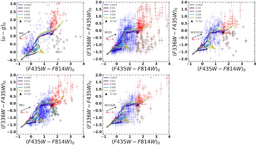
The U-selected cluster candidates in (u − g)0 versus (F435W − F814W)0 diagram for M81 and (F336W − F435W)0 versus (F435W − F814W)0 diagram for the rest of the sample galaxies. Candidates having (F435W − F814W)0 >1.5 mag are GC candidates (red dots), and bluer objects are young disc SSC candidates (blue dots). The evolutionary loci of SSPs from Bruzual & Charlot (2003) for different metallicities using Kroupa IMF are shown by solid curves of different colours, following the colour notation shown in each panel. The bluest colour that a classical GC can have (Z = 0.0004 and age 12 Gyr) is marked by a solid triangle. The reddening vector with AV = 1 mag is shown. The reddened young SSCs that occupy the GC colours are contaminants, which are identified by red dots surrounded by circles of cyan colour.
In Fig. 10, we explore whether contaminant fraction in our GC samples depends on the colour and magnitude of the GCs. We carry out this analysis in bins of 0.5 mag in colours and magnitudes. In order to avoid fluctuations caused due to small number statistics in some of the bins, we plot only those values for which the number of contaminants in any bin was more than the Poisson error in that bin, taken as the square root of the total number of GC candidates in that bin. For the rest of the bins, we plot the global values. In general, all galaxies have higher contaminant fraction for (F435W − F814W)0 >2.2 mag, with as much as 50 per cent of the GCs of (F435W − F814W)0 = 2.5 mag being contaminants (reddened young SSCs) in M101 and M81. None of the galaxies show any significant dependence of the contaminating fraction with magnitude. We hence use the global values of the contaminant fraction to correct the LF obtained from our entire GC sample in Section 5 for all galaxies.
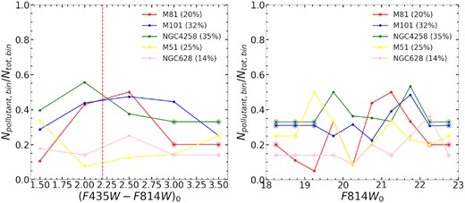
The fraction of contaminants (reddened young SSCs) in our GC samples as a function of colour (left-hand panel) and magnitude (right-hand panel) for our five sample galaxies. The vertical dashed-line in the left-hand figure corresponds to the reddest colours reached by SSPs for unreddened GCs. See the text for details.
3.6 Comparison of our GC catalogues with those in the literature
In four of our five sample galaxies, there exists a previous catalogue of GCs. We reiterate that none of these catalogues are as complete as our catalogues in terms of spatial and magnitude coverages, as well as in the estimation of contamination fraction from reddened SSCs. We here compare our catalogues, obtained using uniform selection criteria, with the catalogues from other authors, using different selection criteria.
3.6.1 M81
Nantais et al. (2010b) reported a sample of 233 GC candidates in M81, that had made use of data from HST/ACS and SDSS. They used an FWHM>3 ACS pixel (0.15 arcsec) as the main discriminator. We find that 107 of our 154 GCs are present in the catalogue of Nantais et al. (2010b). Most of the remaining 49 GCs in our sample have 2.4<FWHM<3 pixel, which is the main reason for their exclusion in Nantais et al. (2010b). Lower number of GCs in our sample as compared to that of Nantais et al. (2010b) is due to the more stringent filtering that we imposed in the selection of GCs.
3.6.2 M101
Similarly, using data from the HST/ACS, Simanton et al. (2015) reported a sample of 326 star clusters in M101. The selection was made using the concentration index and a colour cut. Their sample includes extended objects, and hence they used a magnitude cut of MV ≤ −6.5 to define GCs, resulting in a sample of 98 GC candidates. We find that 48 are present in their sample of GC candidates. Reasons for us missing 50 of their objects are that 25 of these have ELLIPTICITY>0.3, 19 do not meet the AREA criterion and the rest do not meet our FWHM criterion.
3.6.3 NGC 4258
González-Lópezlira et al. (2017) reported a sample of 39 GCs in NGC 4258 using near-infrared (NIR) data from CFHT (Canada–France–Hawaii Telescope) over a large FoV (1° × 1°), but based on seeing-limited (∼0.7 arcsec) data set. The selection of the GCs was carried out using the colour–colour diagram u*i′Ks ((i′ − Ks) versus (u* − i′)) (Muñoz et al. 2014). In comparison, our catalogue using HST/ACS images contains 226 GCs over an FoV of ∼12.3 arcmin × 17.2 arcmin. From a spectroscopic follow-up of the objects, González-Lópezlira et al. (2019) concluded that the selection based on colour–colour diagram has between 10 and30 per cent contaminants (e.g. Muñoz et al. 2014; González-Lópezlira et al. 2019). Our FoV includes 29 objects of González-Lópezlira et al. (2017), of which 23 are in our catalogue. Out of the six missing objects in our sample, two are confirmed to be GCs using spectroscopic data by González-Lópezlira et al. (2019), another two are dwarf galaxies, with the remaining one being a foreground star. Reason for the two of their GCs to be absent in our sample is that they do not satisfy our selection criteria.
3.6.4 M 51
Star clusters in M51 were catalogued by Hwang & Lee (2008) using HST/ACS images. They used the SExtractor parameters stellarity, FWHM, and ellipticity for star cluster selection. They created two subsamples, one with 2.4<FWHM<20 and the other with 2.4<FWHM<40 pixel, resulting in a catalogue of 8400 stellar cluster candidates. If we applied their colour discriminator ((B − V) >0.5 and (V − I) >0.8) in their catalogue we obtained a sub-catalogue of 224 red clusters, 214 of which have FWHM<10 ACS ACS pixels. Only 85 of these objects are in our catalogue of 223 GCs. We searched our master SExtractor output catalogue to find out the reasons for we missing 139 of their objects, and found that 85 of these have ELLIPTICITY>0.3, 15 do not meet the AREA criterion, and the rest do not meet our FWHM criterion.
3.6.5 NGC 628
The last galaxy of our sample, NGC 628, has also been a target for cluster searches using HST images by Ryon et al. (2017). However, they reported only young and intermediate-age clusters, and no GCs.
4 COMPLETENESS CORRECTIONS
We aim to study GC luminosity functions in our sample galaxies. In order to do that, we need to take into account possible sources of incompleteness in our catalogues. Two principal sources of incompleteness in our study are: (i) incompleteness in magnitude and (ii) incompleteness in radial coverage even with multiple HST pointings. In this section, we describe the method we have followed to correct for these observational limitations and obtain a final GC luminosity function.
4.1 Monte Carlo cluster simulations
We generated mock clusters using the iraf/daophot tasks addstars and mkobjects. A cluster is defined by an intensity profile that follows a Gaussian function of a given fwhm and a total magnitude, with fwhm taking values of 2.0, 2.4, 3.0, 4.0, 5.0, 6.0, 7.0, and 8.0 pixels, and magnitudes varying between 19 and 24 magnitudes at interval of 0.5 mag. For a fixed fwhm, 1100 clusters were generated, 100 for each simulated magnitude.
Coordinates of these sources were randomly selected and were inserted on to an observed HST image. The faintest object that can be detected in an observation under uniform background conditions defines the detection limit of that observation. In real observations, the background is often non-uniform, and each non-point source has a different size. Further, crowding of objects in an image can lead to non-detection of objects that are brighter than the detection limit. Hence, for each galaxy, we chose HST images corresponding to two FoV, representing zones of (i) low background and low crowding, and (ii) high background and high crowding. The former simulates the conditions typical of clusters in the external parts of galaxies, whereas the latter represents the characteristics of clusters in the bulge and spiral arms. For M81, which has as many as 29 pointings, simulations were carried out on an additional frame containing the bulge and nucleus (R09; see fig. 1 in Santiago-Cortés et al. 2010, for the footprint of M81). The results of these latter simulations were used exclusively in the analysis of radial density distribution of clusters in the inner part of this galaxy. The same object detection and selection criteria (Section 3.2) we had used for real objects were applied on the mock-object added frames. In Fig. 11, we zoom-in on a randomly selected region of M101, before (left-hand panel) and after (right-hand panel) inserting mock sources. In the image the positions of the mock sources, which cover a range of magnitudes, are indicated by blue circles.
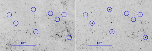
A randomly selected region of M101 before adding mock sources (left-hand panel) and after adding them (right-hand panel); sources have different magnitudes. All blue circular regions have 1 arcsec radius. North up, east left.
We have also used these simulations to establish criteria to select cluster candidates from all sources catalogued by the SExtractor, and apply fwhm-dependent aperture corrections, described in Section 3.3. We used the results of the simulations for low background and low crowding for this purpose.
4.2 Completeness corrections: magnitude
For a proper counting of a population, it is necessary to know completeness factor as a function of object magnitude. We used the results of our simulation to determine the completeness factors. This factor is expected to depend on the fwhm.
In the top panel of Fig. 4, we plot the distribution of fwhm, which peaks at fwhm<3 pixel. Hence, we calculate the completeness factors for mock clusters of input fwhm = 3 pixel. The completeness factor is defined as the ratio of the number of recovered objects (Nout) to the inserted objects (Nin) at each inserted magnitude.
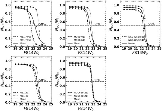
Completeness correction curves in the F814W band for our sample galaxies in low (dotted line passing through circles) and high (dashed line passing through triangles) background regions. The mean of these two curves is shown by the solid line. The identification codes of high and low background frames used in these simulations are shown in parenthesis.
Magnitude at 50 per cent completeness in F814W band, for three curves in Fig. 12.
| Galaxy | Low | High | Average | |||
|---|---|---|---|---|---|---|
| m50 | α | m50 | α | m50 | α | |
| M81 | 22.93 | 3.74 ± 0.01 | 21.65 | 2.15 ± 0.04 | 22.32 | 1.08 ± 0.14 |
| M101 | 22.72 | 3.79 ± 0.00 | 22.11 | 2.69 ± 0.16 | 22.44 | 2.05 ± 0.17 |
| NGC 4258 | 22.60 | 4.02 ± 0.01 | 22.26 | 3.02 ± 0.00 | 22.46 | 2.96 ± 0.13 |
| M51 | 22.92 | 3.24 ± 0.01 | 22.45 | 2.19 ± 0.00 | 22.69 | 2.07 ± 0.06 |
| NGC 628 | 22.85 | 4.01 ± 0.01 | 22.72 | 3.97 ± 0.00 | 22.79 | 3.83 ± 0.01 |
Note. m50 is the magnitude at 50 per cent completeness and α is a fitting constant defined in equation (1).
4.3 Completeness corrections: radial distribution
While the images obtained from HST observations offer the best spatial resolution, they do not cover the whole extent of galaxies even with the multiple pointings. Thus, outer halo GCs are often missing in catalogues selected from HST images. The following analysis was carried out to correct for the absence of GCs beyond the galaxy’s disc.
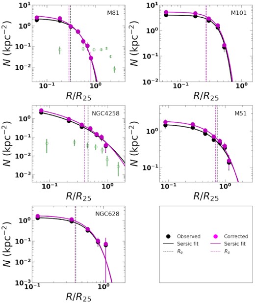
Radial distribution of surface number density of GCs from our data (solid circles) are fitted with Sérsic profile (solid line). Catalogued GCs beyond the spatial coverage of the HST images are shown by the empty circles (M81 and NGC 4258, only). Observed number densities in these two galaxies are consistent with the extrapolation of the fitted function. The vertical dashed lines show the best-fitting values of Re before (black solid circles) and after (magenta solid circles) incompleteness correction.
Results of Sérsic profile fits to the radial distribution of GC surface density.
| Galaxy | Observed | Completeness-corrected | ||||||
|---|---|---|---|---|---|---|---|---|
| n | Re | |$N_{{\rm GC},R_{\rm e}}$| | |$N_{{\rm GC},R_{\rm e}}^\prime$| | n | Re | |$N_{{\rm GC},R_{\rm e}}$| | |$N_{{\rm GC},R_{\rm e}}^\prime$| | |
| (kpc) | (kpc) | |||||||
| M81 | 0.57 ± 0.07 | 4.29 ± 0.16 | 93 ± 11 | 74 ± 9 | 0.66 ± 0.12 | 4.04 ± 0.23 | 109 ± 5 | 87 ± 4 |
| M101 | 0.33 ± 0.05 | 7.68 ± 0.28 | 635 ± 24 | 432 ± 16 | 0.36 ± 0.07 | 7.61 ± 0.32 | 802 ± 15 | 545 ± 10 |
| NGC 4258 | 1.81 ± 0.50 | 9.48 ± 2.02 | 179 ± 39 | 116 ± 25 | 1.63 ± 0.30 | 8.21 ± 0.96 | 197 ± 27 | 128 ± 17 |
| M51 | 0.74 ± 0.15 | 10.07 ± 1.15 | 250 ± 31 | 188 ± 23 | 0.71 ± 0.12 | 9.54 ± 0.78 | 301 ± 20 | 226 ± 15 |
| NGC 628 | 0.48 ± 0.08 | 6.08 ± 0.27 | 113 ± 7 | 97 ± 6 | 0.48 ± 0.09 | 5.95 ± 0.29 | 149 ± 4 | 128 ± 3 |
Note. Re is the effective radius enclosing half the population, n is the Sérsic index from equation (2). |$N_{{\rm GC},R_{\rm e}}$| is the total number of GCs inside Re, whereas |$N_{{\rm GC},R_{\rm e}}^\prime$| is |$N_{{\rm GC},R_{\rm e}}$| after taking into account contamination from reddened young SSCs.
The number density obtained wide-field ground-based surveys underestimates the number of GCs inside Re by more than an order of magnitude in both the galaxies with such data. In NGC 4258, the slope of our fit in the external part agrees with the observed number densities from wide-field survey, with the absolute values marginally below our predictions. On the other hand, number densities obtained from wide-field survey in M81 remain constant over a large radial range, which are likely due to some selection biases in the survey. On the other hand, the wide-field survey suggests an excess of GCs in the external parts of this galaxy as compared to our predicted values. This excess could be due to contamination from foreground stars and unbound intergalactic GCs in the M81 group (see e.g. Jang et al. 2012; Ma et al. 2017).
Two of the most well-studied spiral galaxies, the Milky Way and M31, have n = 1.9 and Re = 4.41 kpc and n = 1.6 and Re = 4.59 kpc (Battistini et al. 1993), respectively. In comparison, for elliptical galaxies the calculated values are larger, e.g. NGC 720 (E5): n = 4.16 ± 1.21, Re = 13.7 ± 2.2 kpc; NGC 1023 (S0): n = 3.15 ± 2.85, Re = 3.30 ± 0.9 kpc; NGC 2768 (E): n = 3.09 ± 0.68, Re = 10.6 ± 1.8 kpc (Kartha et al. 2014). The n and Re for our sample galaxies are in the range of expected values in spiral galaxies. The n values are <1 in four of our galaxies, suggesting flatter distribution in the inner parts of our galaxies, as compared to the Milky Way and M31.
5 GLOBULAR CLUSTER LUMINOSITY FUNCTIONS (GCLFS)
Having obtained a sample of GCs in five spiral galaxies, we now analyse the properties of the GC systems in these galaxies. All magnitudes and colours have been corrected for the foreground Galactic extinction using the AV values given in Table 1, and the Cardelli, Clayton & Mathis (1989) reddening curve. We start our analysis with the colour distribution.
5.1 Colour distribution
For comparing colours of our GCs with those in the MW, we transformed all our photometry into the Johnson–Cousins photometric system using the transformation equation (B1) and the corresponding coefficients in Table B1 in Appendix B, which were taken from Sirianni et al. (2005).
In Fig. 14, we show the distributions of (B − I)0, (B − V)0 and (V − I)0 colours of GC systems in our sample galaxies, where the sub-index 0 stands for Galactic reddening-corrected colours, using the AV values in Table 1. For comparison, we also plot the colour histograms of the GCs in the Milky Way using the data from Harris (1996). The black and blue histograms correspond to the observed and dereddened colours, respectively. In Table 9, we list the mean and mode of the distributions of the three colours (B − I)0, (B − V)0, and (V − I)0 for our sample as well as for the MW sample from Harris (1996). We use only 97 Galactic GCs which had integrated colours available in Harris (1996). For comparison, we list the colour of an SSP of 13 Gyr with Z = 0.001, the typical metallicity of old GCs, in the last row. The reddening-corrected colours of MW GCs agree within 0.1 mag with these SSP colours.

Colour distributions of GCs of our galaxies compared to that in the MW (bottom-most panels). The distributions of (B − I)0 colour after correcting for contaminating fractions are shown by magenta histograms. The mean value for each distribution is shown by a vertical dashed line. The colour histograms after dereddening the colours by the reddening reported for each GC for the MW GCs are shown in blue.
The mean and mode of the colour distribution of sample galaxies and the MW.
| Galaxy | (B − I)0 | (B − V)0 | (V − I)0 | AV(int) | AV(int) | |||
|---|---|---|---|---|---|---|---|---|
| Mean | Mode | Mean | Mode | Mean | Mode | Mean | Mode | |
| (1) | (2) | (3) | (4) | (5) | (6) | (7) | (8) | (9) |
| M81 | 2.21 | 1.81 | 1.31 | 1.21 | 0.90 | 0.77 | 0.86 | 0.32 |
| M101 | 2.49 | 1.68 | 0.96 | 0.65 | 1.54 | 0.98 | 1.23 | 0.15 |
| NGC 4258 | 2.02 | 1.64 | 0.92 | 0.81 | 1.11 | 0.87 | 0.60 | 0.10 |
| M51 | 2.04 | 1.71 | 0.93 | 0.87 | 1.10 | 1.03 | 0.68 | 0.19 |
| NGC 628 | 2.11 | 1.58 | 0.72 | 0.63 | 1.39 | 1.00 | 0.73 | 0.01 |
| MW | 2.34 | 1.70 | 1.01 | 0.72 | 1.33 | 1.01 | 1.04 | 0.17 |
| SSP | 1.57 | 0.67 | 0.90 | |||||
Note. (1) Galaxy name. (2–7) Mean and statistical mode of the indicated colours. (8–9) Internal visual extinction obtained from mean and mode (B − I)0.
The mode is systematically bluer than the mean in all the three colours in our sample galaxies as well as in the MW. This difference is due to a noticeable skewness in the colour distributions, with the peak (mode) occurring on the bluest bin in (B − I)0 and (V − I)0, in all cases except in M81. The skewness is not due to a colour cut we have used to define GCs. In fact the choice of the cut-off colour between SSCs and GCs corresponds to the saddle point in the distribution of colours of all cluster candidates (see Fig. 7), with the peak in the GC colours occurring in the first or second bin redward of the saddle point. We analyse the possible role of contaminants in our GC samples to the origin of skewness in colour distributions. For this, we use the fraction of contaminants as a function of colour (see left-hand panel in Fig. 10) to correct statistically the (B − I)0 colour histograms, which is shown in Fig. 14 in magenta. The contamination-corrected histograms maintain the blue skewness in the distribution. This suggests that the skewness in colour distribution is an intrinsic property of the GC systems.
The mean and mode colours of our GC systems should correspond to SSP colours of metal-poor old clusters, if reddening is negligible. We find that the mode is only marginally redder than the colours of the metal-poor SSPs at old ages, whereas the mean is much redder. The redward shift of the mode from the expected SSP colours and the long red tail of the colour distribution, even for the MW sample, illustrate that the GC colours are often reddened by dust. The typical reddening experienced by GCs in each of our sample galaxies can be determined by comparing the mode of the colour distribution with the colour of the metal-poor old SSPs. We made use of the (B − I)0 colour to obtain the colour excess AV(int) = ((B − I)0 − (B − I)SSP)/(EB − EI), where (B − I)SSP is the (F435W − F814W)0 colour of the SSP, EB = 1.33, and EI = 0.60 are the values of the thardelli et al. (1989) extinction curve at the effective wavelengths of B and I bands. The resulting values of AV(int) using mean and mode are given respectively in columns 8 and 9 of Table 9. The AV(int) obtained from the mode for our galaxies range from 0.01 (NGC 628) to 0.32 mag (M81) which is comparable to the 0.17 mag for the MW. The AV(int) values obtained from the mean colours vary between 0.60 (NGC 4 258) and 1.23 (M101), which is also comparable to the 1.04 mag for the MW.
The difference between the mean and median AV values is ∼0.5–1.0 in our sample galaxies, which is comparable to that for the Milky Way (0.87). Thus, GC systems in spiral galaxies experience relatively large mean extinctions. In fact, this is one of the reasons for the slow progress in establishing the properties of the GC systems in spiral galaxies. Some of the reddening could be due to dust internal to the clusters, whereas the majority is expected due to the dust along the line of sight in the disc of the host galaxy. The colour histogram in M101 shows a second peak at (B − I)0 ∼3.5 mag after correction for contaminants, suggesting the presence of a distinct red population. The analysis of LF below also suggests the presence of a population fainter than GCs. As we will see in Section 5.4, this population of faint red clusters corresponds to reddened intermediate age (1–10 Gyr) SSCs. Under such a scenario, the basic assumption we have made in determining AV, namely the clusters are old (>10 Gyr) is not applicable to all clusters in M101 and hence the AV(mean) would be an upper limit for this galaxy.
5.2 Luminosity function
We chose the Galactic extinction-corrected magnitudes in the F814W band to construct the GCLF. For this purpose, we constructed histograms in bins of 0.5 mag over the entire range of detected magnitudes for each galaxy. The resulting histograms are shown in Fig. 15 with red solid lines. The magnitudes corresponding to 50 per cent completeness, m50, at low and high surface brightness parts of for each galaxy are shown by dotted and dashed vertical lines, respectively. The observed numbers are corrected for incompleteness using the mean function shown in Fig. 12. The corrected histograms are shown by grey bars. As expected, the correction factor is negligible at the bright end (F814W ≲ 21 mag), and gradually increases at fainter magnitudes.
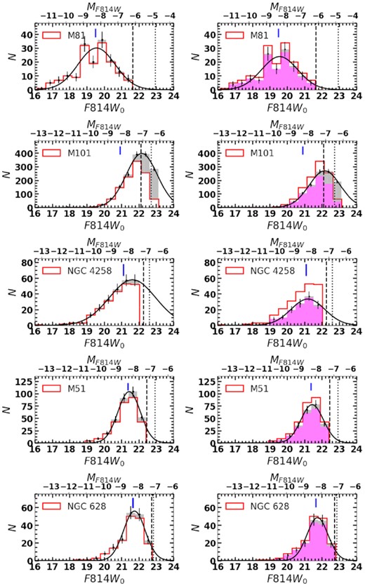
Best lognormal fits to the observed F814W-band luminosity functions of GCs in our five sample galaxies. The data before (red histograms) and after (magenta-filled histograms) correction for possible contamination from reddened young SSCs are shown in the left-hand and right-hand panels, respectively. In each panel, fits were carried out to the completeness-corrected data set (grey-filled histograms). Poisson error bars (|$\sqrt{N}$|) are indicated. The vertical dot and dashed lines indicate the magnitude at which the detection is 50 per cent complete at low and high surface brightness parts of the galaxies, respectively. For reference, the turnover magnitude for the MW GCs is indicated in each plot by the blue vertical bar. The horizontal axes in the bottom and top contain observed and absolute magnitudes, respectively.
We obtained the TO magnitude after correcting the LF in each galaxy for a possible contribution from the contaminants. Following the discussions in Section 3.5, we used the magnitude-dependent contaminant fractions for NGC 4258 and constant contaminant fractions from the last column in Table 5 for the rest. The resulting plots for each galaxy are shown in the right-hand panels of Fig. 15 and the results are tabulated in Table 10. In order to determine the possible errors on the determined TO, we carried out 1000 Monte Carlo simulations, by adding a Gaussian noise to each bin of the histograms. For this purpose, we used the square root of the number in each bin as the σ of the Gaussian. The histogram resulting from each experiment is fitted by equation (3), each time finding TO and σM. The rms values of these 1000 simulations are taken as the error on TO and σM.
Number of GCs and best-fitting values for a lognormal distribution.
| Galaxy | NGC | TO | ΔTO | σM | Δσ | |$M_{814}^{1^{st}}$| | |$M_{814}^{3^{rd}}$| | ||||
|---|---|---|---|---|---|---|---|---|---|---|---|
| Obs | ∫LF | total | F814W0 | M|$_{F814W_{0}}$| | M|$_{V_{0}}$| | ||||||
| (1) | (2) | (3) | (4) | (5) | (6) | (7) | (8) | (9) | (10) | (11) | (12) |
| M81 | 126 | 128 ± 13 | 177 ± 15 | 19.56 ± 0.12 | −8.42 ± 0.13 | −7.52 ± 0.16 | −0.12 | 1.04 ± 0.17 | −0.11 | −11.66 | −10.84 |
| M101 | 764 | 1325 ± 60 | 1891 ± 70 | 22.16 ± 0.05 | −7.14 ± 0.08 | −6.24 ± 0.13 | 1.16 | 0.89 ± 0.05 | −0.26 | −11.57 | −10.10 |
| NGC 4258 | 147 | 166 ± 31 | 290 ± 51 | 21.19 ± 0.11 | −8.26 ± 0.11 | −7.36 ± 0.15 | 0.04 | 0.97 ± 0.15 | −0.18 | −11.57 | −11.40 |
| M51 | 220 | 261 ± 24 | 536 ± 44 | 21.44 ± 0.07 | −8.34 ± 0.07 | −7.44 ± 0.12 | −0.04 | 0.64 ± 0.05 | −0.51 | −10.76 | −10.35 |
| NGC 628 | 149 | 151 ± 16 | 259 ± 18 | 21.75 ± 0.05 | −8.21 ± 0.06 | −7.31 ± 0.12 | 0.09 | 0.60 ± 0.07 | −0.55 | −11.66 | −10.23 |
Note. (1) Galaxy name. (2) Number of GCs after correcting for contamination from reddened SSCs. (3) Column 2 after correcting for incompleteness in magnitude. (4) Estimated total number of GCs determined using equation (6). (5) Observed TO magnitude in F814W-band. (6) TO absolute magnitude in F814W-band, corrected for galactic and internal extinction. (7) TO absolute magnitude in V-band (|$M_{V_{0}}$| = |$M_{F814W_{0}}$|+(V − I)SSP; (V − I)SSP = 0.90). (8) ΔTO = TO(galaxy)-TO(MW) in the V-band, where TO(MW) = −7.4 mag. (9) σM, from the fit. (10) Δσ = σM(galaxy)−σ(MW), where σ(MW) = 1.15). (11) |$M_{814}^{1^{\rm st}}$|, magnitude of the brightest GC. (12) |$M_{814}^{3^{\rm rd}}$|, magnitude of third brightest GC.
In order to investigate the universality of the function, we converted the apparent TO magnitudes to the absolute values using the best-available distances for the sample galaxies (see Table 1), and corrected these magnitudes for internal extinction using AF814W(int) = 0.58AV(int), where AV(int) is taken from the last column of Table 9. The resulting values are also given in Table 10. All galaxies with the exception of M101 are consistent with MI0 = −8.21 ± 0.06 mag, with a mean MV0 = −7.41 ± 0.14 mag. The TO of M101 is 1.16 mag fainter. We will discuss this case separately in next section.
How does the mean value for the galaxies compare with the values for elliptical galaxies and the MW? TO value for the MW is MV = −7.40 ± 0.10 mag (from Jordán et al. 2007), which is almost identical to the mean value of MV0 = −7.41 ± 0.14 mag obtained for four of our galaxies. The individual differences of the TO magnitudes for our sample galaxies from that of the MW are given in column 8 of the Table 10. The differences are well within 1σ value in all these four galaxies. Hence, the GCLFs in four of our sample galaxies have the same TO as that in the MW. In comparison, M31 value of MV0 = −7.60 ± 0.15 obtained by Secker (1992) and Reed et al. (1994) is ∼0.2 mag brighter than our mean value, which is marginally larger than the 1-σ error of our measurements. As pointed out earlier, TO for M101 is clearly different, which could be due to underestimation of distance, or an intrinsically different value of TO. This will be analysed in detail in the next sub-section.
Despite the near universality of the TO values, the σM of the lognormal function varies widely in the sample galaxies. These differences in widths are illustrated in Fig. 16, where we plot all the lognormal fits normalized to their peak values. The TO value along with its error for the Milky Way GCs is shown as a vertical band. In this figure, we also show the positions of the brightest GC in each of these galaxies, as well as the position of the third brightest GC. It can be easily seen that the dispersion in the brightest and the third brightest clusters in these galaxies is much higher than the dispersion in the TO values, suggesting that the TO values are more universal than the magnitude of the brightest, or the third brightest GC, in galaxies. The brightest GC in our sample of five galaxies belongs to M81, which is discussed in detail in Mayya et al. (2013).
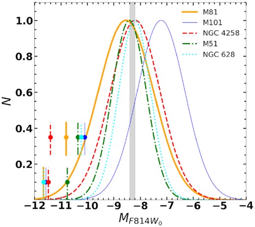
Comparison of the normalized F814W-band GCLFs of all our sample galaxies. Line types and colours used for each galaxy are indicated. The TO magnitude of the MW GCs is marked by the grey band, with its width indicating the error on this value. The dispersion of the TO values in four of the galaxies (M101 is the exception) is smaller than the dispersion of their brightest GCs (bottom-most set of vertical lines) or the third brightest GCs (top set of vertical lines).
5.3 Distance errors and the universality of the TO
For obtaining the TO, we have used the distances tabulated in Table 1. The tabulated distances correspond to the most recent determination of distances using Cepheids for M81 and M101, and the MASER distance for NGC 4258. For M51 and NGC 628, SNII distances were used.
Using only the distances reported after the year 2000 in NED,7 we found 56 independent measurements for M81,8 79 for M101,9 77 for NGC 4258,10 27 for M5111, and 23 for NGC 628.12 The methods of distance measurements include those using Cepheids, MASER, tip of the red giant branch (TRGB), SNII-optical, and Tully–Fisher. We recalculated TO values for each of these measured distances, which are shown plotted against the corresponding distances in Fig. 17. The value of TO for the best-determined distance (that in Table 1) is indicated by a thick circle, which is colour-coded according to the method that was used to obtain the distance. The error on this best measurement is highlighted by the grey band. Most of the distance measurements for the four galaxies (M81, NGC 4258, M51, and NGC 628) agree with the value obtained by our best distance estimate, after taking into consideration the errors on each of them. In M101 where we found TO value fainter by 1.16 mag, some of the Cepheid distances are not consistent with the Cepheid distance (6.95 Mpc) we have used. If we use the farthest distance reported for this galaxy (8.99 Mpc; Macri et al. 2001), the TO value is still 8σ fainter than the universal value we have in other galaxies. Hence, we conclude that the TO value in M101 is intrinsically fainter compared to that in other galaxies of our sample, and investigate the possible physical reasons for this difference.
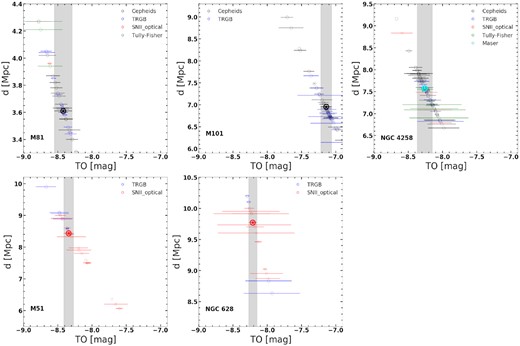
Dependence of the measured TO (circle) on the distance uncertainties. The measurement error on TO is shown by the width of the vertical grey band. Symbols in each plot are colour-coded depending on the method of distance determination.
5.4 TO magnitude in M101 and late-type galaxies
Among the galaxies analysed in this study, M101 stood out from the rest for having a fainter derived TO value, as well as for having a large population of very red clusters ((F435W − F814W)0 >2.2 mag), including a second peak at (F435W − F814W)0 >3.5 mag in its colour distribution (Fig. 14). We here discuss whether these differences are related to its late morphological type (Scd). In Fig. 18, we plot the TO values with respect to that in the MW as a function of the morphological type of the host galaxies. In this plot, we include the MW, M31, and the Large Magellanic Cloud (LMC). We estimated the TO in the LMC using data from Mackey & Gilmore (2003) for clusters with age ≥1 Gyr. TO values in all galaxies with morphological type Sc or earlier are in agreement with the value in the MW within the errors of measurements. The two galaxies later than Sc deviate from this trend. Thus, there is an indication that the different TO value found in M101 is indeed related to its late morphological type. In the following paragraphs, we discuss a possible scenario that naturally explains the fainter TO in late-type galaxies.
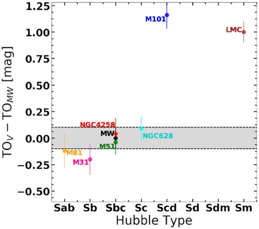
TOV −TOMW versus the Hubble Type of host galaxies. The plot includes our five sample galaxies, and other spiral (M31) and irregular (LMC) galaxies where such measurements are available. The error in the MW TO is indicated by the width of the grey band.
Classical GCs are among the oldest objects in galaxies, and their formation is related to the formation of halo and bulge (Brodie & Strader 2006). By definition, the prominence of these spherical components in galaxies decreases along the Hubble sequence. For this very reason, most of the searches of GCs were traditionally carried out in elliptical and early-type galaxies. Such studies have found relatively larger population of classical GCs in ellipticals as compared to that in spiral galaxies (e.g. Harris & Harris 2011; Harris, Harris & Alessi 2013). On the other hand, M101 has a weak bulge, classified as a pseudobulge by Kormendy et al. (2010), and a very poor stellar halo population (Jang et al. 2020), as expected for its late morphological type. These late-type systems are not expected to contain a large population of classical GCs. However, searches of GCs on HST images, including this study, find as many GCs in late-type galaxies as in early-type spirals. It is likely that not all the inferred GCs in late-type galaxies are classical GCs. We analyse this issue below.
Spiral and irregular galaxies are known to contain old SSCs that were formed in their discs and have survived the tidal shocks of their host galaxies. For example, González-Lópezlira et al. (2019) found that some of the objects classified as GCs in NGC 4258, one of the galaxies analysed in our study, belong to its disc and share the same kinematics as the disc H i gas. Formation and growth of galaxies through hierarchical merging, expects formation of such clusters during every epoch of merger involving gas-rich galaxies (Mamikonyan et al. 2017). The selection filters used for GC searches on HST and ground-based images do not distinguish these old stellar clusters from the classical GCs. Thus generally speaking the sample of objects observationally classified as GCs contains two kinds of objects, classical GCs related to the spherical component of galaxies, and old disc star clusters, formed in-situ or accreted onto, during galaxy mergers as part of the hierarchical growth of galaxies. It is the former one that is expected to have universal TO. The fraction of old star clusters is expected to increase towards later Hubble types as they are more gas-rich than the early types. Hence, the TO obtained in early-type spirals represents that of the classical GCs, whereas in late-type galaxies it represents the population of old SSCs in the disc. This is found to be true in the LMC, where 50 per cent of the old cluster population that is used to obtain the TO has ages in the 1–10 Gyr range.
In Section 3.5, we have estimated the contamination fraction from reddened SSCs in our sample of GCs in each galaxy, using the photometry in the U-band. The technique we have used helps us to distinguish reddened SSCs from GCs only for SSCs younger than ∼3 Gyr. Thus, our GC samples, in principle, contain all clusters older than ∼3 Gyr. The universality of the TO in all our galaxies earlier than Sc, suggests that these early-type spirals did not form significant amount of SSCs after the formation of halo and bulge, or even if they are formed, they did not survive the gravitational shocks.
The GC population in M101 has been the subject of study by Simanton et al. (2015). They found a total of 326 candidate GCs, with their luminosity function matching very well the LF for the Galactic GCs, but starts increasing rapidly for MV ≥ −6.5 mag. They identified these relatively fainter clusters as belonging to a second population, which is statistically more extended than the brighter population, the so-called faint fuzzies (e.g. Larsen & Brodie 2000b; Brodie & Larsen 2002; Peng et al. 2006; Liu et al. 2016). They discuss these red extended clusters as old stellar clusters formed in the disc. Only 98 (i.e. 30 per cent) of their clusters belonged to the brighter population, the classical GCs. Our selection criteria, which selects objects 2.4<FWHM<10 pixel, naturally rejects extended objects that Simanton et al. (2015) have found, but contains compact objects fainter than their magnitude cut of MV ≥ −6.5 mag. The fainter TO we have found suggests that our sample is dominated by a population of red faint compact clusters of ages between ∼1–10 Gyr. These properties correspond to relatively low-mass reddened SSCs in the disc of M101.
5.5 Physical parameters that control TO
Physical parameters corresponding to TO.
| Galaxy | Z | Age | |$\mathcal {M}_{\rm cl}$|/M⊙ | σ |
|---|---|---|---|---|
| Gyr | log | log | ||
| M81 | 0.0004 | 13.0 | 5.58 | 0.05 |
| 0.001 | 13.0 | 5.57 | 0.05 | |
| M101 | 0.0004 | 13.0 | 5.07 | 0.03 |
| 0.001 | 13.0 | 5.06 | 0.03 | |
| NGC 4258 | 0.0004 | 13.0 | 5.52 | 0.04 |
| 0.001 | 13.0 | 5.51 | 0.04 | |
| M51 | 0.0004 | 13.0 | 5.55 | 0.02 |
| 0.001 | 13.0 | 5.54 | 0.02 | |
| NGC 628 | 0.0004 | 13.0 | 5.50 | 0.02 |
| 0.001 | 13.0 | 5.49 | 0.02 | |
| MW | 0.0004 | 13.0 | 5.53 | 0.04 |
| 0.001 | 13.0 | 5.52 | 0.04 |
5.6 Total number of globular clusters and specific frequency
GC searches in external galaxies using HST data are subjected to two kinds of incompleteness: (i) magnitude incompleteness arising due to the missing low-luminosity GCs beyond the detection limit, and (ii) area incompleteness due to non-coverage of outer-halo GCs because of the limited FoV of HST. The alternative strategy of searching GCs in wide-field ground-based surveys also suffers from these two effects, with the second effect arising due to confusion with stellar sources in the inner regions due to lack of spatial resolution. Characterization of the LF and the radial number density distributions with analytical functions, allows us to calculate the total number of GCs by integrating over the entire range of these functions. We carry out these integrations in two steps, as explained below.
The specific frequency, SN, defined as the number of GCs normalized to the total galaxy magnitude of MV = −15 mag, is related to the NGC, TOT by the relation SN|$={N}_{\rm GC,TOT}\times 10^{0.4({M}_{V}+15)}$| (Harris & van den Bergh 1981). We calculated SN for each galaxy using the MV tabulated in Table 1. In Table 12, we show SN and SN, TOT calculated with NGC, OBS and NGC, TOT, respectively. In Fig. 19, we show the SN, TOT versus MV. We also show corresponding values for the MW and M31 (Peacock et al. 2010). The value of SN for M101 is expected to be an upper limit, given that our GC sample for this galaxy includes a large population of intermediate-age SSCs. We hence made an alternative estimation of SN, assuming that the true GC population in this galaxy also has the universal TO. We hence counted the number of GCs brighter than MV = −7.40 mag, and doubled that number to calculate NGC, TOT. The empty symbol for M101 in the figure corresponds to this revised SN. The mean value for our sample, including the revised value of M101 is ∼1.10 ± 0.24, which occupies a much smaller range as compared to the values for spiral galaxies from the compilation of Harris et al. (2013) (open circles). The large spread in the latter sample is expected as they are based on studies using very different detection and analysis techniques from Fischer et al. (1990), Harris (1996), Kissler-Patig et al. (1999), Harris & Harris (2000), Goudfrooij et al. (2003), Olsen et al. (2004), Rhode & Zepf (2004), Rhode et al. (2007), Di Nino et al. (2009), Mora et al. (2009), Nantais et al. (2010a), Peacock et al. (2010), Rhode, Windschitl & Young (2010), Adamo et al. (2011), and Young et al. (2012).
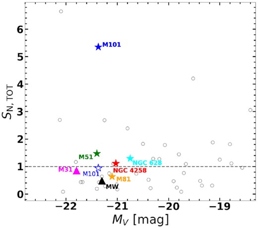
GC specific frequency plotted against the absolute magnitude of the host galaxy for our sample of five galaxies (filled star symbol), the MW and M31 (triangles). The empty star symbol for M101 corresponds to the value obtained assuming a universal TO for this galaxy (see the text for details). The dashed horizontal line indicates average values for spiral galaxies from the compilation of Harris et al. (2013), which are shown by empty circles.
Specific frequency.
| Galaxy | SN | SN, TOT |
|---|---|---|
| M81 | 0.46 ± 0.10 | 0.64 ± 0.10 |
| M101† | 2.16 ± 0.46 | 5.35 ± 0.82 |
| NGC 4258 | 0.57 ± 0.26 | 1.12 ± 0.30 |
| M51 | 0.61 ± 0.17 | 1.48 ± 0.22 |
| NGC 628 | 0.75 ± 0.17 | 1.30 ± 0.24 |
| Galaxy | SN | SN, TOT |
|---|---|---|
| M81 | 0.46 ± 0.10 | 0.64 ± 0.10 |
| M101† | 2.16 ± 0.46 | 5.35 ± 0.82 |
| NGC 4258 | 0.57 ± 0.26 | 1.12 ± 0.30 |
| M51 | 0.61 ± 0.17 | 1.48 ± 0.22 |
| NGC 628 | 0.75 ± 0.17 | 1.30 ± 0.24 |
Note. †Values estimated assuming the universality of TO applies to M101 are 0.47 ± 0.27 and 0.94 ± 0.33.
6 CONCLUSIONS
We used the HST images of five nearby spiral galaxies for which there are data taken with multiple pointings with ACS to enable a search of GCs in them. Images in F435W, F555W, and F814W filters were used. We used SExtractor and a set of cluster-defining filters to define a sample of GCs in each of the analysed galaxies. Detection of simulated clusters was carried out to obtain the incompleteness as a function of magnitude. We used the U-band photometry for a subset of sample GCs using the SDSS u-band images for M81 and HST/WFC3 F336W images for the rest to evaluate the contamination of our GC samples by reddened SSCs. The contaminating fraction was found to be between 0.14 and 0.35. We used the data set to construct luminosity function of GCs in spiral galaxies.
We find that the LF of GCs in all the five galaxies analysed is lognormal in nature, with the turn-over (TO) happening on the brighter side of the 50 per cent incompleteness limit in all galaxies. This has enabled us to determine precise TO magnitudes for our sample of galaxies. We also determined typical internal extinction towards the population of GCs in our sample galaxies by comparing the mode of the observed colours with that from population synthesis models for a metal-poor (metallicity = 1/20th solar) population of 13 Gyr. We used the best determined distances for the sample galaxies to convert the extinction corrected V-magnitude corresponding to the turn-over into the absolute magnitude MV0(TO) and obtained errors on this by carrying out Monte Carlo simulations. The mean of the MV0(TO) in four of our galaxies is −7.41 ± 0.14, which is in excellent agreement with the values determined for GC population in the Milky Way of MV0(TO)MW = −7.40 ± 0.10. In the fifth galaxy M101, MV0(TO) is 1.16 mag fainter than that for the MW. We propose that this difference in MV0(TO) arises due to morphological differences, with spiral galaxies of the Hubble types Sc or earlier having a universal MV0(TO), whereas the Hubble types later than Sc have fainter MV0(TO). The universality of MV0(TO) in early-type spirals is due to the classical GCs dominating the GC population, whereas in late-type spirals GC population is often dominated by old disc clusters, which are in general less massive, and hence fainter than the classical GCs, but otherwise share the same observational properties as the classical GCs. The universal TO value corresponds to a stellar mass of ∼3 × 10⁵ M⊙, where the corresponding value is a factor of 2 lower for M101.
We used the data set of GCs to address three other topics of interest, namely the form of the radial density distribution, distribution of colours, and the specific number density. The Sérsic function with index between n = 0.36–1.63 is a good fit for the radial density distribution of GCs in our sample of galaxies. The index value suggests exponential form, rather than the much steeper n = 3–4 form found in elliptical galaxies (Kartha et al. 2014). We carried out a statistical analysis of (B − I)0, (B − V)0 and (V − I)0 colour distributions for our sample of five galaxies. We found that the correction factor for contaminating reddened SSCs is a function of GC colour. Taking into account the errors in this correction factor, we find no compelling evidence for a bimodal distribution. We have calculated NGC, the total number of GCs by making corrections for undetected faint sources, and those outside of our FoV, by extrapolating the GCLF to fainter magnitude and radial surface density profiles to outside our FoV, respectively. The specific number density SN∼1.10 ± 0.24 for our sample of spiral galaxies.
SUPPORTING INFORMATION
Table 6. Observational properties of the all GCs in each sample galaxy.
Please note: Oxford University Press is not responsible for the content or functionality of any supporting materials supplied by the authors. Any queries (other than missing material) should be directed to the corresponding author for the article.
ACKNOWLEDGEMENTS
We are grateful to two anonymous referees for their valuable suggestions on the original manuscript, especially for suggesting us to carryout corrections for possible contamination of our GC samples from reddened young clusters. LLN thanks Consejo Nacional de Ciencia y Tecnología (CONACyT) for granting PhD research fellowship that enabled him to carry out the work presented here. We also thank CONACyT for the research grants CB-A1-S-25070 (YDM), and CB-A1-S-22784 (DRG).
Based on observations made with the NASA/ESA Hubble Space Telescope, and obtained from the Hubble Legacy Archive, which is a collaboration between the Space Telescope Science Institute (STScI/NASA), the Space Telescope European Coordinating Facility (ST-ECF/ESA) and the Canadian Astronomy Data Centre (CADC/NRC/CSA).
This research has made use of the NASA/IPAC Extragalactic Database (NED) which is operated by the California Institute of Technology, under contract with the National Aeronautics and Space Administration.
This work has made use of data from the European Space Agency (ESA) mission Gaia (https://www.cosmos.esa.int/gaia), processed by the Gaia Data Processing and Analysis Consortium (DPAC, https://www.cosmos.esa.int/web/gaia/dpac/consortium). Funding for the DPAC has been provided by national institutions, in particular the institutions participating in the Gaia Multilateral Agreement.
DATA AVAILABILITY
Table 6 in it is complete form is available as online suplementary material. The reduced fits files on which these data are based will be shared on reasonable request to the first author.
Footnotes
The zeropoints were obtained from ACS Zeropoints Calculator: https://acszeropoints.stsci.edu/.
REFERENCES
APPENDIX A: COMPARISON WITH THE HLA CATALOGUES
We started our work using the SExtractor catalogues for cluster selection, available at the Hubble Legacy Archive (HLA). With our method of selection, we expect that an object has at least AREA = 50 pixels to be considered as candidate for a star cluster. We found that AREA values reported in HLA catalogues: 02, a2, and 11 of M101 are very small, with very few objects having AREA > 50 pixel. On other fields of the same galaxy, there were sources having AREA > 50 pixel. In order to understand the absence of sources having AREA > 50 pixel, we downloaded the images and ran the SExtractor using the same input file as that used by the HLA.
In top Fig. A1, we show a comparison between MAG_ISO (top row) and AREA (bottom row) of HLA catalogues and SExtractor catalogues obtained by us in F814W-band. The histograms of both the quantities compare very well. However, HLA MAG_ISO is systematically fainter and the AREA systematically smaller than the values we obtained, and hence the observed differences in fields 02, a2, 11 for M101 can be directly understood in terms of an underestimation of background in the HLA catalogues.
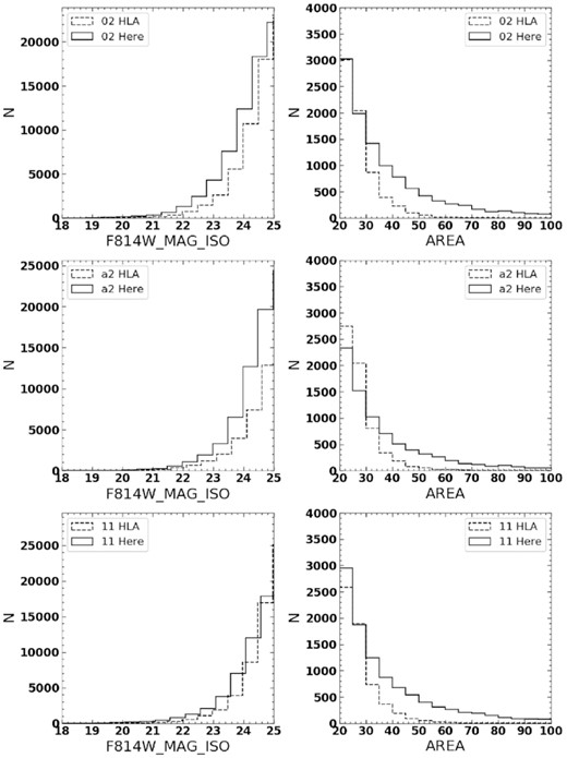
Frames covering M101 with incorrect values of AREA and MAG_ISO values in the source catalogues of HLA. The frame numbers for set are indicated. Dashed histograms show the values from the HLA catalogues, whereas the solid histograms show values from our catalogue, using the same SExtractor input file as for the HLA catalogue.
The distribution of the SExtractor parameters available at HLA coincided with that obtained from our own runs of SExtractor for all other frames where we made a comparison. However, in order to ensure uniform analysis of all sample galaxies, we downloaded the fits files and generated our own catalogues for each frame. The discussion presented here serves as a cautionary note while planning to use the HLA catalogues for quantitative scientific studies.
APPENDIX B: TRANSFORMATION TO JOHNSON–COUSINS SYSTEM
Transformation coefficients between HST and Johnson–Cousins systems.
| HST | UBVRI | TCOL | c1 | c2 | Range |
|---|---|---|---|---|---|
| F435W | B | B − I | 0.022 ± 0.006 | −0.038 ± 0.011 | <1.0 |
| F435W | B | B − I | 0.008 ± 0.006 | −0.005 ± 0.001 | >1.0 |
| F555W | V | B − V | −0.083 ± 0.032 | 0.020 ± 0.115 | <0.2 |
| F555W | V | B − V | −0.087 ± 0.007 | 0.004 ± 0.002 | >0.2 |
| F814W | I | B − I | 0.013 ± 0.006 | −0.028 ± 0.112 | <0.3 |
| F814W | I | B − I | −0.010 ± 0.010 | −0.006 ± 0.002 | >0.3 |
| F606W | V | B − V | 0.170 ± 0.005 | 0.061 ± 0.002 | ... |
