


ABSTRACT
We present redshift-space two-point (ξ), three-point (ζ), and reduced three-point (Q) correlation of Lyα absorbers (Voigt profile components having H i column density, NH i > 1013.5 cm−2) over three redshift bins spanning 1.7 < z < 3.5 using high-resolution spectra of 292 quasars. We detect positive ξ up to 8 h−1 cMpc in all three redshift bins. The strongest detection of ζ = 1.81 ± 0.59 (with Q = 0.68 ± 0.23) is in |$z$| = 1.7–2.3 bin at 1–2 h−1 cMpc. The measured ξ and ζ values show an increasing trend with NH i, while Q remains relatively independent of NH i. We find ξ and ζ to evolve strongly with redshift. Using simulations, we find that ξ and ζ seen in real space may be strongly amplified by peculiar velocities in redshift space. Simulations suggest that while feedback, thermal and pressure smoothing effects influence the clustering of Lyα absorbers at small scales, i.e. <0.5 h−1 cMpc, the H i photoionization rate (ΓH i) has a strong influence at all scales. The strong redshift evolution of ξ and ζ (for a fixed NH i cut-off) is driven by the redshift evolution of the relationship between NH i and baryon overdensity. Our simulation using best-fitting ΓH i(|$z$|) measurements produces consistent clustering signals with observations at |$z$| ∼ 2 but underpredicts the clustering at higher redshifts. One possible remedy is to have higher values of ΓH i at higher redshifts. Alternatively the discrepancy could be related to non-equilibrium and inhomogeneous conditions prevailing during He ii reionization not captured by our simulations.
1 INTRODUCTION
The intergalactic medium (IGM) manifests itself in the form of Lyα forest absorption in the spectra of distant bright sources (quasars, galaxies, and γ-ray bursts). The observed properties of these absorption features are governed by the matter distribution in the IGM along with its thermal and ionization state. The baryonic content of the IGM is known to trace the underlying dark matter density fluctuations at large scales; while at small scales, it experiences some additional smoothing due to the gas pressure (see Bi & Davidsen 1997). Majority of the baryons exist in a photoionized low-density (i.e. typical overdensity, Δ, in the range 1–10 at 2 < |$z$| < 4) state in the IGM at high redshifts. In the post-H i reionization era (|$z$| < 6), the ionization state of the low-density H i gas in the IGM and its evolution are determined by a uniform metagalactic ultraviolet background (UVB; Haardt & Madau 1996, 2012; Khaire & Srianand 2015, 2019; Oñorbe, Hennawi & Lukić 2017; Puchwein et al. 2019; Faucher-Giguère 2020). The thermal state of this photoionized low-density gas (decided mainly by H i and He ii reionization) and its evolution are well studied and the existence of a temperature–density (T–Δ) relation is well established (see Hui & Gnedin 1997).
The IGM studies are generally based on observational data in conjunction with hydrodynamical simulations. In particular, for a given set of cosmological and astrophysical parameters, the physical conditions are derived using the observed properties of Lyα forest such as, neutral hydrogen column density (NH i) distribution, Doppler parameter (b) distribution, mean transmitted flux probability distribution function (PDF), wavelet and curvature statistics, and flux power spectrum (see Cen et al. 1994; Petitjean, Mueket & Kates 1995; Zaldarriaga 2002; Springel 2005; Becker et al. 2011; Smith et al. 2011; Bolton et al. 2012; Garzilli et al. 2012; Rudie, Steidel & Pettini 2012; Boera et al. 2014; Gaikwad et al. 2017a,b, 2020, 2021). Besides understanding the astrophysical properties of IGM, Lyα forest spectra have been useful in constraining cosmological parameters (Viel et al. 2004a; Viel, Haehnelt & Springel 2004b; McDonald et al. 2005) and placing bounds on masses of warm dark matter particles (Viel et al. 2013; Iršič et al. 2017) and neutrino (Palanque-Delabrouille et al. 2015a,b, 2020; Yèche et al. 2017).
A quintessential role in understanding the matter distribution in the IGM is played by the clustering studies of Lyα forest. Most of these studies focused on redshift-space clustering using several quasar spectra and transmitted flux (longitudinal correlation or power spectrum in Fourier space; see McDonald et al. 2000, 2006; Croft et al. 2002; Seljak, Slosar & McDonald 2006). One can also study clustering in the transverse direction between adjacent sightlines (transverse correlation) of closely spaced projected quasar pairs or gravitationally lensed quasars (Rauch & Haehnelt 1995; Smette et al. 1995; Petitjean et al. 1998; Aracil et al. 2002; Coppolani et al. 2006; D’Odorico et al. 2006; Hennawi et al. 2010; Rollinde et al. 2013; Maitra et al. 2019). Transverse correlation statistics based on transmitted flux is found to be more sensitive to the 3D baryonic distribution in comparison to longitudinal correlation, which is affected primarily by thermal broadening effects (Peeples et al. 2010a,b). However, due to sparsity of projected quasar pairs, the transverse studies are relatively scant in number. Nevertheless, they have been helpful in constraining the pressure broadening scales in IGM that is known to be sensitive to the thermal history of the Universe (Kulkarni et al. 2015; Rorai et al. 2017).
Higher order clustering studies in Lyα forest are useful in probing non-Gaussianity in the matter density distribution caused by non-linear gravitational evolution. While three-point clustering (using three-point correlation, or bispectrum in Fourier space) has been studied largely at low redshifts using galaxies (Gaztanaga & Frieman 1994; Gaztañaga & Scoccimarro 2005; Sefusatti et al. 2006; Kulkarni et al. 2007; McBride et al. 2011a,b; Guo et al. 2016) or at higher redshifts for large scales using quasars (de Carvalho et al. 2020), Lyα forest as an observable would be able to probe the matter clustering at smaller scales and at higher redshifts. In addition to constraining the second-order quadratic bias in clustering, three-point statistics can also act as an independent tool along with the two-point statistics in constraining cosmological parameters (Fry 1994; Verde et al. 2002) and the physical state of IGM. In fact, Mandelbaum et al. (2003) had shown that three-point statistics in Lyα forest along with two-point statistics can determine the amplitude, slope, and curvature of the slope of the matter power spectrum with better precision. It has also been pointed out three-point statistics is helpful in removing degeneracies between different cosmological parameters like the bias and amplitude of matter power spectrum (Bernardeau et al. 2002; Verde et al. 2002).
Nevertheless, three-point statistics in Lyα forest remains largely unexplored. A few studies have been performed in exploring three-point statistics using cross-correlation between Lyα forest power spectrum and matter density field probed by cosmic microwave background (CMB) weak-lensing signal (Doux et al. 2016; Chiang & Slosar 2018). Viel et al. (2004a) had used a large sample of Ultraviolet and Visual Echelle Spectrograph (uves) quasi-stellar object (QSO) absorption spectra (luqas) and found that the error bars in the observed bispectrum (redshift space) of Lyα forest (at 2.0 ≤ |$z$| ≤ 2.4) transmitted flux were too large to distinguish them from a set of absorption spectra having randomized absorber positions. For the past 3 yr we have been exploring using the Voigt profile components of the Lyα absorption to study two- and three-point correlation function of the IGM (Maitra et al. 2019, 2020a,b). We have shown that such an approach allows us to study the clustering properties as a function of NH i and b parameters.
Maitra et al. (2020b) had explored low-|$z$| Lyα forest (|$z$| < 0.48) using the Hubble Space Telescope (HST)/Cosmic Origins Spectrograph (COS) data (of Danforth et al. 2016) and had detected longitudinal three-point correlation in Lyα absorbers for the first time with a 2.6σ significance. While detailed analysis of redshift-space three-point correlation is possible, studies of transverse three-point correlation using close projected quasar triplets are still mostly at theoretical stages (Tie et al. 2019; Maitra et al. 2020a) due to scarcity of bright targets. There are still some attempts to study higher order clustering properties of Lyα forest using few projected quasar triplets at high-|$z$| (Cappetta et al. 2010; Maitra et al. 2019).
Here, we use a large sample of high-resolution (∼6 |$\mathrm{km\, s}^{-1}$|) QSO spectra from a publicly available Keck Observatory Database of Ionized Absorption toward Quasars (KODIAQ)survey data Release 2 (DR2;O’Meara et al. 2015, 2017) and UVES Spectral Quasar Absorption Database (SQUAD) survey Data Release 1 (DR1; Murphy et al. 2019) to study the longitudinal (redshift-space) three-point correlation of Lyα forest along high-z quasar sightlines. Similar to Maitra et al. (2020b), we will be using the Voigt profile components (denoted as absorbers in this paper) based approach of decomposing the Lyα forest absorption into distinct Voigt profile components and calculate the two- and three-point correlation for them. The large size of this sample also allows us to probe the redshift evolution of these correlation functions.
This paper is organized as follows. In Section 2, we describe the final sample of Lyα forest used for our analysis. In Section 3, we provide details of the hydrodynamical simulations used to interpret our observational results. In Section 4, we present details of completeness of our sample as a function of NH i and the H i column density distribution separately for KODIAQ and SQUAD data. This exercise is important to establish the internal consistency between the two data sets. Then using the combined data set we present the NH i distribution for three different redshift bins of our interest. In Section 5, we present our measurements of two- and three-point correlation for the three redshift bins (i.e. 1.7 < |$z$| < 2.3, 2.3 < |$z$| < 2.9, and 2.9 < |$z$| < 3.5) from observations. In this section, we also present the H i column density dependence of the correlation functions and how metal line contamination affects our measurements. We also present our clustering measurements in a tabulated form for future use. In Section 6, using simulated spectra, we quantify how the measured clustering is affected by (1) H i photoionization rate (ΓH i), (2) pressure broadening effects (or the so-called Jeans smoothing), (3) line-of-sight (LOS) peculiar velocities (or redshift-space distortions), and (4) feedback processes. In Section 7, we discuss the redshift evolution of clustering. We show the strong evolution observed is mainly dominated by evolution in the physical state of the IGM and discuss the possible evolution in ΓH i that can explain the observed evolution. Our results are summarized in Section 8.
2 OUR SAMPLE OF HIGH-z Lyα ABSORBERS
In this work, we use two publicly available compilations of high-resolution (i.e. ∼6 |$\mathrm{km\, s}^{-1}$|) quasar spectra to study the clustering properties of high-|$z$| (i.e. 1.7 ≤ |$z$| ≤ 3.5) Lyα absorbers. The first sample is from the KODIAQ-DR2 (O’Meara et al. 2017).1 KODIAQ-DR2 sample consists of spectra of 300 quasars at 0.07 < |$z$|em < 5.29 obtained with Keck/High Resolution Echelle Spectrometer (HIRES) at high resolution (|$30\,000\le R \le 103\,000$|). Just for uniformity we consider only spectra having spectral resolution R ∼ 40 000–45 000. In the case of KODIAQ, individual spectra of a target observed multiple times are available. In such cases we have co-added them following the procedure described in appendix A in Gaikwad et al. (2021). Additionally, we also use quasar spectra from the publicly available DR1 of the SQUAD comprising fully reduced and continuum fitted high-resolution spectra of 467 quasars at 0 < |$z$|em < 5 observed using Very Large Telescope (VLT)/UVES (Murphy et al. 2019).2
As we are mostly interested in the IGM studies, we do not consider a spectrum that contains damped Lyα (DLA; systems with log NH i ≥ 20.3) or sub-DLA (i.e. systems with 19 ≤ log NH i ≤ 20.3) systems and associated broad absorption line (BAL) systems. For this we manually scanned all the spectra in the combined sample. We also cross-checked the emission redshifts quoted in these data sets. We check for duplicate quasar spectra between the two samples (i.e. SQUAD and KODIAQ) and considered the spectrum having higher median signal-to-noise ratio (SNR) and better wavelength coverage for our study. We also removed spectrum with a median spectral SNR per pixel <5 in the Lyα forest region. The final list of number of quasar spectra used, redshift range, and median SNR are summarized in Table 1. This yields 213 quasar spectra from KODIAQ and 77 quasar spectra from SQUAD covering Lyα forest in the range of 1.7 < |$z$| < 3.5. For our study we consider the Lyα absorption spectra between the Lyα and Lyβ emission lines of the quasar and excluding 10 h−1 pMpc proximity region close to the quasar. The details of these sightlines (quasar name, emission redshift, absorption redshift range considered for our study, and the median SNR in this range) are given in Tables A3 and A4 in Appendix A (provided as supplementary material).
Details of our Lyα sample used in this study.
| Redshift interval | Redshift path-length | Number of LOS | Median SNR | ||||
|---|---|---|---|---|---|---|---|
| KODIAQ | SQUAD | KODIAQ | SQUAD | KODIAQ | SQUAD | KODIAQ+SQUAD | |
| 1.7–2.3 | 16.19 | 16.32 | 110 | 59 | 10.4 | 11.7 | 11.2 |
| 2.3–2.9 | 19.69 | 7.28 | 143 | 26 | 12.0 | 20.7 | 13.1 |
| 2.9–3.5 | 11.40 | 5.07 | 82 | 18 | 14.1 | 20.3 | 15.5 |
In order to probe the redshift evolution of the clustering, we divide the data in to three different subsamples based on the redshift range covered by the Lyα absorption. We consider redshift bins of width δ|$z$| = 0.6 centred around |$z$| = [2.0, 2.6, 3.2]. Details of the subsample: total redshift path-length without correcting for sensitivity, number of quasar sightlines considered, and the median SNR of the subsample are summarized in Table 1 for the two data sets discussed above. It can be seen from this table that in the 1.7 ≤ |$z$| ≤ 2.3 bin the redshift path-length for both samples is similar despite KODIAQ sample containing double the number of quasar sightlines. This is because redshift interval covered by individual quasar sightline in KODIAQ is typically less than that of squad in this redshift bin (see Tables A3 and A4). Detailed description of the redshift path-length corrected for detection sensitivity for a given NH i is provided in Section 4.
In our analysis, we do not remove the metal line contamination in the Lyα forest. To quantify the effect of metal line contamination in the measured clustering, we consider two subsamples in the low-|$z$| (37 quasar sightlines probing 1.9 ≤ |$z$| ≤ 3.1 Lyα forest in the squad sample) and high-|$z$| bins (18 quasar sightlines probing 2.9 < |$z$| < 3.5 Lyα forest in the squad sample). In both cases we manually checked the available spectra for the presence of strong metal absorption systems through C iv, Si iv, and Mg ii doublets. After identifying these systems we systematically looked for associated metal line absorption that falls within the wavelength range of interest for our Lyα absorption studies. We then masked these contaminating lines. We note that strongest contamination originates from strong metal lines having absorption components spread over few hundred |$\mathrm{km\, s}^{-1}$|. We find the metal line contamination does not influence our clustering measurements and results of this exercise are presented in Section 5.4.
For our analysis, we decompose the observed Lyα absorption spectrum into multiple Voigt profile components using the automated profile fitting routine viper (see Gaikwad et al. 2017b, for details). We use only absorption lines that are detected above 3σ significant levels. In what follows we call the individual Voigt profile component as ‘absorbers’. In the series of studies we have highlighted the advantage of using ‘absorbers’ for the clustering analysis (refer to discussions in Maitra et al. 2019, 2020a,b) compared to most frequently used flux-based statistics.
In this work, we also consider different cosmological simulations to understand the measured clustering properties of the Lyα absorbers. Before discussing our measurements we provide details of simulations used in our study in the following section.
3 SIMULATION OF Lyα FOREST SPECTRA
We have run hydrodynamical simulations using gadget-3 code, which is a modified version of the publicly available code gadget-23 (Springel 2005) based on smoothed particle hydrodynamics (SPH). The modified code self-consistently incorporates radiative heating and cooling processes in the thermal and ionization evolution equation, thereby simulating the physical properties of the IGM more accurately. The description of the simulation run and the procedure of forward modelling the simulated particle properties along sightlines to produce the transmitted flux are given in the following subsections (see also, Maitra et al. 2020a).
3.1 Description of simulation
We have generated a (100 h−1 cMpc)3 simulation box with 2 × 10243 particles for a uniform metagalactic UVB (Khaire & Srianand 2019). We use a standard flat Λ cold dark matter (ΛCDM) cosmology with cosmological parameters based on Planck Collaboration XVI (2014) ([ΩΛ, Ωm, Ωb, h, ns, σ8, Y] ≡ [0.69, 0.31, 0.0486, 0.674, 0.96, 0.83, 0.24]). The initial condition for the simulations are generated at |$z$| = 99 using 2lpt4 (Scoccimarro et al. 2012) code, which evolves the density fields based on second-order Lagrangian perturbation theory. We take the gravitational softening length to be 1/30th of the mean interparticle separation. We also turn on the quick_lyalpha flag in the simulation, which makes the simulation run faster by converting gas particles with overdensity Δ > 103 and temperature T < 105 K to stars (see Viel et al. 2004a). The simulations do not incorporate feedback processes sourcing from active galactic nuclei (AGN) or supernovae-driven galactic winds.
We use two different simulation runs for this work. The fiducial model has been run with Khaire & Srianand (2019)5 metagalactic UVB having a far-ultraviolet (UV) quasar spectral index α (fν ∝ ν−α) of 1.8. We also use a simulation run with an enhanced thermal history. In this case, we artificially double the background photoheating rates with a uniform heat injection for all the particles independent of their densities, while keeping the photoionization rates same. In doing so, we not only increase the temperature of the baryon field at mean overdensity, but also puff up the baryonic matter distribution due to increased gas pressure. The redshift evolution of the parameters related to thermal and ionization state of the gas [temperature at mean baryonic overdensity (|$T_0$|), power-law index (γ − 1) of the temperature–density relation (T = T0Δγ − 1), and H i photoionization rate (ΓH i)] for our ‘fiducial’ simulation (α = 1.8) and ‘hot’ simulation with enhanced UVB (enhanced α = 1.8) has been plotted in panels (a)–(c) of Fig. 1. As can seen, ΓH i is same for the two simulations and because of the uniform heat injection, γ also remains more or less similar. The main difference between the ‘fiducial’ and ‘hot’ box is that the temperature is about ∼1.5 times higher in the hot case.
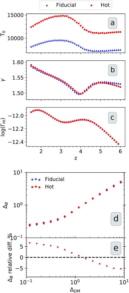
Panels (a)–(c) show the redshift evolution of temperature at mean baryonic overdensity (|$T_0$|), power-law index (γ) of the temperature–density relation, and H i photoionization rate (ΓH i), respectively, for our ‘fiducial’ ‘hot’ simulations (see Section 3 for details). Panel (d) shows the baryon–dark matter overdensity relation seen in the two simulation boxes at |$z$| = 2.0. In panel (e), we plot the relative difference between the two distributions that quantifies the effect of additional pressure smoothing experienced by the baryons in the ‘hot’ simulations.
To understand the effect of baryonic pressure smoothing between the two boxes, we shoot 4000 random sightlines through both the boxes for |$z$| = 2.0 snapshot. We calculate the 1D dark matter and baryonic overdensities (ΔDM and ΔB, respectively) along these sightlines using a standard Cloud-in-Cell algorithm for dark matter field and SPH smoothing for baryonic field over 4096 grids. We then bin the ΔDM values logarithmically in the range of 0.1–10 and find the median ΔB corresponding to each ΔDM bin for 4000 sightlines. We plot the ΔDM versus ΔB relation in panel (d) of Fig. 1 for the ‘fiducial’ and ‘hot’ simulation box. In panel (e), we plot the relative percentage differences in ΔB at each ΔDM bin for the ‘hot’ model with respect to our ‘fiducial’ model. In the underdense regions (ΔDM ∼ 0.1), the ΔB corresponding to ‘hot’ model is higher than that for the ‘fiducial’ model by 7 per cent. In the overdense regions (ΔDM ∼ 10), the ΔB corresponding to the ‘hot’ model is less by 5 per cent. The fact that the overdense region becomes less overdense and underdense region becomes less underdense shows the enhanced pressure smoothing effect in the baryonic density fields for the ‘hot’ model. Thus, we will use both our simulation boxes to investigate the effect of the thermal state of the gas and pressure smoothing effects on the clustering properties of Lyα absorbers.
Note that in Maitra et al. (2020a), we found the relative difference in ΔB is very small when we consider UVB models with allowed range in power-law spectral index for the quasar spectral energy distribution (SED; see their fig. 14 for details). From the measurements presented in Gaikwad et al. (2021), we find the value of T0 to in the range (0.95–1.45) × 104 K for the redshift range of our interest. Our ‘hot’ model typically produces higher T0 values and hence the actual pressure smoothing effects may be smaller than that of our ‘hot’ model.
Additionally, we will also use two hydrodynamical simulation boxes from publicly available Sherwood simulation6 suite (Bolton et al. 2017) to study the effect of wind and AGN feedback on the Lyα clustering at |$z$| ∼ 2.0. Both these simulations were performed in an 80 h−1 cMpc cubic box with 2 × 5123 particle using P-Gadget-3 (Springel 2005). The ‘80–512’ model is run with quick_lyalpha flag (as described in Viel et al. 2005) without any stellar or wind feedback. The second simulation ‘80–512–ps13+agn’ implements the star formation and energy-driven wind model of Puchwein & Springel (2013) and the AGN feedback. Both simulations have same initial seed density field, utilize Haardt & Madau (2012) UVB, and use the same set of cosmological parameters from Planck Collaboration XVI (2014), where Ωm = 0.308, ΩΛ = 0.692, Ωb = 0.0482, h = 0.678, σ8 = 0.829, ns = 0.961. As can be seen these are very close to the cosmological parameter used for our simulations discussed above.
3.2 Forward modelling of Lyα forest spectra
We shoot random sightlines through the simulation box that contains particle information such as overdensity (Δ), peculiar velocity (|$v$|), and temperature (T). We then use SPH smoothing to get 1D Δ, |$v$|, and T fields along these sightlines. We employ this SPH smoothing by sampling over 4096 uniform grids along box length. The choice of this gridding scheme is to keep the pixel size of the simulated spectra similar to the observations. To compute the H i density (nH i) along a sightline, we consider two choices of ΓH i.
The ΓH i from Khaire & Srianand (2019) that is the default photoionizing background in our simulation boxes. We refer to this as ΓKS19. We use this while exploring the effects of various astrophysical parameters on clustering of Lyα absorbers in simulations.
The ΓH i obtained by matching the observed and simulated mean transmitted fluxes, which we will refer to as Γobs. We use this while comparing simulated statistics with the observed ones.
Using the nH i, |$v$|, and T fields, we calculate the Lyα optical depth τ as a function of wavelength along these sightlines (see equation 30 of Choudhury, Srianand & Padmanabhan 2001). The Lyα transmitted flux is computed as a negative exponential of τ. In the case of Sherwood simulations, we sample over a sparser 2048 uniform grids, since the number of particles is lesser than our simulation box. We do not use these simulations for comparing the simulated statistics with observation, but rather to investigate the effect of wind and AGN feedback only. For the Sherwood simulations, we have rescaled optical depths with the ΓH i from Khaire & Srianand (2019) UVB model.
To mimic the observed spectra, we first convolve the simulated transmitted flux with an instrumental Gaussian with a full width at half-maximum (FWHM) value of ∼6 |$\mathrm{km\, s}^{-1}$| (i.e. the typical instrumental resolution of Keck/HIRES and VLT/UVES). We then add a Gaussian random noise to the flux to mimic the observed noise properties. Similar to ΓH i, we make two choices for generating noise along the sightlines.
Gaussian random noise corresponding to a uniform SNR of 50 pixel−1. We will refer to this as |$\rm SNR_{50}$| and will use it while exploring the effects of various astrophysical parameters on clustering of Lyα absorbers in simulations. We will typically use this in conjunction with ΓKS19 photoionizing background.
Gaussian random noise based on the observed SNR distribution across the sightlines in our KODIAQ and SQUAD sample. We randomly draw a value from the observed distribution of median SNR in a given redshift bin, and then assign that value uniformly across a simulated sightline. We repeat this procedure for all the sightlines. We will refer to this as |$\rm SNR_{obs}$| and will use it while comparing simulated statistics with the observed ones, typically in conjunction with Γobs.
Finally, we also decompose the simulated Lyα forest transmitted flux into distinct Voigt profile components using viper (Gaikwad et al. 2017b). We then use the ‘absorber’ list created by viper for our clustering analysis.
4 OBSERVED H i COLUMN DENSITY DISTRIBUTION
In Fig. 2, we plot the ‘sensitivity curve’ showing the total redshift path-length (Δ|$z$|) over which the absorption produced by the gas having H i column density NH i can be detected at more than 3σ level for the KODIAQ and SQUAD samples in the three redshift bins. The coloured ticks on the sensitivity curve denote the log NH i value corresponding to completeness at the level of 99 per cent. We find that logNH i = 13.5 is more than 99 per cent complete in all the redshift bins. So, for our study, we only consider Lyα absorbers having NH i > 1013.5 cm−2. For this column density limit we get the redshift path-lengths close to those summarized in Table 1.
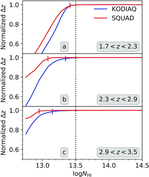
Sensitivity curve showing the total redshift path-length (Δ|$z$|) as a function of logNH i for the KODIAQ (blue curves) and SQUAD (red curves) samples in the three redshift bins. The curve has been normalized to 1 for 100 per cent completeness limit. The coloured ticks on the sensitivity curve denote the logNH i value corresponding to completeness at the level of 99 per cent. We find that logNH i = 13.5 is more than 99 per cent complete (vertical dotted line) in all the redshift bins. We use this value as a minimum NH i threshold for studying clustering of Lyα absorbers. Total redshift path-length covered for each redshift for this NH i threshold is provided in Table 1.
In Fig. 3, we plot the NH i distribution for the KODIAQ and SQUAD samples separately for the three redshift bins of |$z$| = [1.7–2.3, 2.3–2.9, and 2.9–3.5]. The error in the distribution is estimated using two methods: one-sided Poissonian uncertainty in the number of absorbers corresponding to ±1σ and bootstrapping error computed over all the sightlines for a given redshift bin. The larger of the two errors is taken to be the error associated with the distribution. The NH i distribution is similar between the two samples within the error bars. The figure also clearly reveals the redshift evolution in the distribution. The number of absorbers in the lower NH i bin decreases and in the higher NH i bins increases with increasing redshift. We compare our NH i distributions with those obtained by Kim et al. (2013) in two redshift bins: |$z$| = 1.9–2.4 and 2.4–3.2 using 18 high-resolution, high-SNR quasar spectra obtained from the ESO VLT/UVES archive. We find reasonable agreement between our NH i distribution and that of Kim et al. (2013) for the 2.3 ≤ |$z$| ≤ 2.9 bin. However, in the 1.7 < |$z$| < 2.3 bin we do see our values are slightly higher than those of Kim et al. (2013).
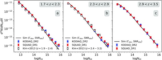
The NH i distribution of Lyα absorbers in the KODIAQ and SQUAD data sample at three different redshift bins. The errors correspond to larger of the two errors: one-sided Poissonian uncertainty in the number of absorbers corresponding to ±1σ or bootstrapping error about the mean distribution. The hollow dots represent measurements by Kim et al. (2013) in two redshift bins: |$z$| = 1.9–2.4 and 2.4–3.2. The black curves represent NH i distribution from our fiducial simulation obtained by matching observed mean transmitted flux and having random Gaussian noise similar to the observed SNR distribution.
As a sanity check for our simulations, we also plot the NH i distribution obtained using the forward modelled sightlines for our fiducial simulation (with Γ = Γobs and |$\rm SNR=SNR_{obs}$|) at |$z$| = 2.0, 2.6, and 3.2 in Fig. 3. The simulated and observed distributions match well with each other in all the three redshift bins. However, we do find that the simulations to slightly underproduce the number of high column density (i.e. log(NH i) ≥ 15.0) absorbers at |$z$| = 2.0 and 2.6 in comparison to the KODIAQ and SQUAD samples.
In Fig. 4, we plot the NH i distribution from the combined KODIAQ+SQUAD sample for the three redshift bins. These values are tabulated in Table A1 in Appendix A. We find indications for evolution of the NH i distribution. The lowest redshift bin 1.7 ≤ |$z$| ≤ 2.3 has higher number of low NH i absorbers (NH i ∼ 1013 cm−2) in comparison to the 2.9 ≤ |$z$| ≤ 3.5 bin. On the other hand, the highest redshift bin 2.9 ≤ |$z$| ≤ 3.5 has larger number of high NH i absorbers (NH i > 1014 cm−2).

Measured H i column density distribution of Lyα absorbers in the combined KODIAQ+SQUAD data sample at three redshift intervals. The error bars are obtained as explained in Fig. 3.
5 CLUSTERING OF Lyα ABSORBERS
We study the clustering of Lyα absorbers by decomposing the Lyα forest into distinct Voigt profile components. This absorber-based approach allows one to study clustering of the Lyα absorbers as a function of NH i (see Cristiani et al. 1997, for early clustering studies based on Voigt profile Lyα components at high-|$z$|). In this section, we calculate the longitudinal (redshift-space) two-point and longitudinal three-point correlation of absorbers in KODIAQ and SQUAD samples and their dependence on NH i and |$z$|.
5.1 Longitudinal two-point correlation
Since the observed SNR does not vary appreciably along individual sightlines (unlike what we encounter at low-|$z$| in Maitra et al. 2020b), we assume a constant median SNR along each individual sightline while populating the random absorbers for our clustering analysis. The two-point correlation is estimated using 100 random sightlines for each of the data sightline and then by normalizing DD and RR with the total number of data–data (nD) and random–random (nR) pair combinations nD(nD − 1)/2 and nR(nR − 1)/2, respectively. We compute the two-point correlation in logarithmically spaced r∥ bins of [0.125–0.25, 0.25–0.5, 0.5–1, 1–2, 2–4, 4–8, 8–16, 16–32, 32–64] h−1 cMpc.
First, the correlations are calculated separately for NH i > 1013.5 cm−2 absorbers in the KODIAQ and SQUAD samples and compared in panel (a)–(c) in Fig. 5 in the three redshift intervals as a function of longitudinal separation r∥. We calculate the associated errors using two methods: one-sided Poissonian uncertainty in the number of absorber pairs corresponding to ±1σ and bootstrapping error. We take the larger of the two errors to be the error associated with the correlation. It is evident from the figure that the two-point correlation function measured for the two samples match very well for the two highest redshift bins. However in the low-|$z$| bin we see differences in the measurements from the two sample. Note that in this redshift range the data are collected in the blue part of the CCD where the data are typically noisy. Also while the redshift path-length probed for the two samples are nearly same (see Table 1) typical SNR achieved and redshift coverage per sightline in the SQUAD spectra are much higher than that of KODIAQ as can be seen from the appreciable difference in the number of quasar sightline used. We also notice that within the narrow redshift bin the distribution of redshift range covered is also different. The SQUAD sightlines typically probe lower |$z$| than the KODIAQ sightlines.
Absorber-based longitudinal two- and three-point correlation (top to bottom) of Lyα absorbers (NH i > 1013.5 cm−2) as a function of comoving longitudinal scale for three different redshift intervals of interest in this work. The velocity scales corresponding to the comoving longitudinal length scales are indicated in the top abscissa. The correlations are shown for KODIAQ and SQUAD sample separately. The error bar shown corresponds to the larger of the two errors: one-sided Poissonian uncertainty in the number of absorber pairs (or triplets) corresponding to ±1σ or bootstrapping error. Both the sample show significant detections of two- and three-point correlation function.
The two-point correlation has a non-zero amplitude within r∥ = 8 h−1 cMpc at 1.7 ≤ |$z$| ≤ 2.3 and 2.3 ≤ |$z$| ≤ 2.9 redshift bins and within r∥ = 4 h−1 cMpc at 2.9 ≤ |$z$| ≤ 3.5 redshift bin. At scales below 0.25 h−1 cMpc (∼75 |$\mathrm{km\, s}^{-1}$| at |$z$| = 2.0, ∼97 |$\mathrm{km\, s}^{-1}$| at |$z$| = 2.6, and ∼122 |$\mathrm{km\, s}^{-1}$| at |$z$| = 3.2), we find a suppression in the correlation amplitudes at all the redshift bins. This characteristic suppression can be attributed to a lower limit on the scale for identification of multiple Lyα absorption lines set by a finite line width of the thermally broadened absorption along with instrumental resolution and other systematic effects. In Section 6, we explore various physical parameters that can influence the measured two-point correlations at different scales (including the suppression seen at small scales) in detail using simulated data.
Next, we combine the KODIAQ and SQUAD data samples and plot the combined two-point correlation in panels (a)–(c) in Fig. 6. The values are tabulated in Table A2 in Appendix A. We detect positive two-point correlation up to a length scale of r∥ = 8 h−1 cMpc in all the redshift bins. The strongest two-point correlation is seen at r∥ = 0.25–0.5 h−1 cMpc bin at 1.7 ≤ |$z$| ≤ 2.3 with an amplitude of ξ = 1.39 ± 0.11. Strongest correlation is seen in the same r∥ bin for |$z$| = 2.3 ≤ |$z$| ≤ 2.9 and 2.9 ≤ |$z$| ≤ 3.5 too. Their amplitude decreases with increasing redshift (ξ = 1.08 ± 0.09 at |$z$| = 2.3–2.9 and 0.41 ± 0.04 at |$z$| = 2.9–3.5). Our measurements are consistent with the early results of Cristiani et al. (1997) albeit with much better sensitivity and over smaller redshift bins as expected due to the large sample used.
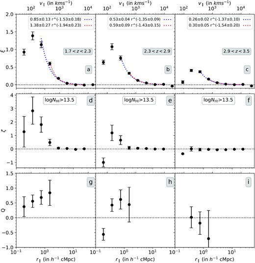
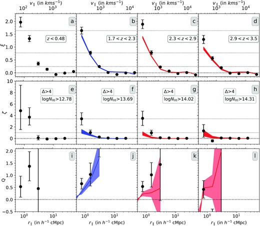
Absorber-based longitudinal two-, three-, and reduced three-point correlation (top to bottom) of Lyα absorbers (NH i > 1013.5 cm−2) as a function of longitudinal scale for three different redshift intervals. The corresponding velocity scales are indicated in the top abscissa. The correlations are shown for combined KODIAQ+SQUAD sample. The error bar shown corresponds to the larger of the two errors: one-sided Poissonian uncertainty in the number of absorber pairs (or triplets) corresponding to ±1σ or bootstrapping error. The coloured dashed curves in the top panels show the power law best fit to the profile of two-point correlation at r∥ > 0.5 h−1 cMpc (blue) and r∥ > 1 h−1 cMpc. In each panel, we also provide the best-fitting power law.
In the top panels of Fig. 6, we fit the observed radial profile of clustering using a power law. As ξ measured at small scales are possibly affected by systematic effects we consider the fit for r > 0.5 and 1.0 h−1 cMpc. The best-fitting values are also shown in each panel. For |$z$| = 2.3–2.9 and 2.9–3.5 the best-fitting values of power-law parameters are consistent within errors on the cut-off value of r∥. Based on these fits we find the ξ(r∥ = 1 h−1 cMpc) = 0.53 ± 0.04 and 0.26 ± 0.02, respectively, for these two redshifts. In the case of |$z$| = 1.7–2.3 bin, it appears that the single power law will not provide adequate fit to all the data above r > 0.5 h−1 cMpc. We find ξ(r∥ = 1 h−1 cMpc) = 0.85 ± 0.13 based on fits to data points at r > 0.5 h−1 cMpc. Thus the observed clustering of Lyα absorbers with log NH i > 13.5 shows strong evolution in amplitude over the redshift range considered. If we approximate the redshift evolution to a power law, then we find roughly ξ ∝ (1 + |$z$|)−3.5. This evolution is much steeper than what is expected purely based on dark matter evolution [i.e. (1 + |$z$|)−5/3; see Cristiani et al. 1997]. We present a detailed discussion on the redshift evolution in Section 7.
The power-law coefficient of radial profile of the two-point function ranges between −1.35 and −1.94. In Maitra et al. (2020a), we found that the radial profile of the simulated two-point function in the longitudinal direction is well approximated by a power law with the index of ∼−0.8. It will be important to confirm such a difference in real data using transverse correlations. In Section 6, we discuss the effect of peculiar velocities on the radial profile.
5.2 Longitudinal three-point correlation
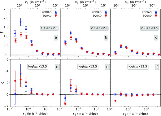
Similar to two-point correlation, we also plot the three-point correlation separately for the KODIAQ and SQUAD samples first as a function of longitudinal separation r∥ in panel (d)–(f) of Fig. 5. The error bars are calculated similar to two-point correlation. Both the samples give similar three-point correlation function in all the redshift bins. Only in the first r∥ bin of |$z$| = 2.3–2.9 and 2.9–3.5 redshift intervals we do find some discrepancy that can come from difference in systematics in the two samples. We combine the two samples and plot the resulting three-point correlation as a function of r∥ in panels (d)–(f) of Fig. 6. We clearly detect three-point correlation at a much higher significant level.
Similar to two-point correlation, the three-point correlation is also largely suppressed in the r∥ = 0.125–0.25 h−1 cMpc bin. At the lowest redshift bin, we detect positive three-point correlation up to a scale of 2 h−1 cMpc. The strongest detections in three-point correlation come at r∥ = 0.25–0.5 and 0.5–1 h−1 cMpc bins (ζ = 2.83 ± 1.02 and ζ = 1.81 ± 0.59, respectively) with a significance of 2.8σ and 3.1σ level. In the intermediate-redshift bin (i.e. 2.3 ≤ |$z$| ≤ 2.9), positive three-point correlation is seen up to a scale of 1 h−1 cMpc only. The three-point correlation values at r∥ = 0.25–0.5 and 0.5–1 h−1 cMpc bins are ζ = 1.19 ± 0.59 and ζ = 0.66 ± 0.35, respectively. In the highest redshift bin (i.e. 2.9 ≤ |$z$| ≤ 3.5), we detect no positive three-point correlation.
5.3 Dependence of NH i threshold
It is well known that the two-point correlation function of both low- and high-|$z$| Lyα absorbers strongly depends on NH i (Cristiani et al. 1997; Penton, Stocke & Shull 2002; Danforth et al. 2016). In our past studies involving redshift-space clustering of low-|$z$| Lyα absorbers in observations (Maitra et al. 2020b) or transverse clustering of |$z$| ∼ 2 absorbers in simulations (Maitra et al. 2020a), we had found that both two- and three-point correlation depend strongly on the NH i of the absorber. Here, we will investigate the NH i dependence of redshift-space two-, three-, and reduced three-point correlation in the three redshift bins: |$z$| = 1.7–2.3, 2.3–2.9, and 2.9–3.5. We do so for three longitudinal scales: r∥ = 0.5–1, 1–2, and 2–4 h−1 cMpc. In case of reduced three-point correlation, we omit the 2–4 h−1 cMpc scale since the signals are very noisy. The results are plotted in Fig. 7.
![Absorber-based longitudinal two-point, three-point, and reduced three-point correlation (top to bottom) of Lyα absorbers as a function of NH i thresholds in different redshift intervals (left to right). The plots are made for scales r∥ = [0.5–1 (blue), 1–2 (red), and 2–4 (green)] h−1 cMpc. The dashed curves represent the power-law fit for the two-point ($\xi =\xi _{14}\mathcal {N}_{14}^{\beta }$, where $\mathcal {N}_{14}$ is the limiting NH i in units of 1014 cm−2) and three-point correlation ($\zeta =\zeta _{14}N_{14}^{\beta }$) as a function of NH i thresholds. The error bars shown correspond to the larger of the two errors: one-sided Poissonian uncertainty in the number of absorber pairs (or triplets) corresponding to ±1σ or bootstrapping error.](https://oup.silverchair-cdn.com/oup/backfile/Content_public/Journal/mnras/509/1/10.1093_mnras_stab3053/1/m_stab3053fig7.jpeg?Expires=1750166103&Signature=1RVPfqjBKe8YaoQOcW1D6kfliNR7nMaXx8aOH~MzltjF9G1PgAdXJVregDdXOOZozvpHy6RPG-72rUckw8gTfJmWYTSfN057ZcEw0folawvdrh5gSp64au10eH0y6WUNVza5O56vx-v2qKqG46rLlFqfwRR5cdRfZrXqB1hfpVSu-8lfQLBOacmQ0LXgErSfokGffNZcPsrNX~91lIzWR-dZN8rFYD-TttkzqwrKp-67SY0I9lUsgEAc4h6Mkv4~REeUlLzGAbimcDd8PiAC37aJU-c5xoJBQ3wxEOOAxz8XSWx-O0cgjtl4ekafW2ZFngRTcQSQFRhqVdArdoWKIg__&Key-Pair-Id=APKAIE5G5CRDK6RD3PGA)
Absorber-based longitudinal two-point, three-point, and reduced three-point correlation (top to bottom) of Lyα absorbers as a function of NH i thresholds in different redshift intervals (left to right). The plots are made for scales r∥ = [0.5–1 (blue), 1–2 (red), and 2–4 (green)] h−1 cMpc. The dashed curves represent the power-law fit for the two-point (|$\xi =\xi _{14}\mathcal {N}_{14}^{\beta }$|, where |$\mathcal {N}_{14}$| is the limiting NH i in units of 1014 cm−2) and three-point correlation (|$\zeta =\zeta _{14}N_{14}^{\beta }$|) as a function of NH i thresholds. The error bars shown correspond to the larger of the two errors: one-sided Poissonian uncertainty in the number of absorber pairs (or triplets) corresponding to ±1σ or bootstrapping error.
We find a strong NH i dependence of both two- and three-point correlation at all scales and in all the redshift bins. To quantify this trend, we fit the NH i dependence of two-point correlation with a power-law fit of the form |$\xi =\xi _{14}\mathcal {N}_{14}^{\beta }$|, where |$\mathcal {N}_{14}$| is limiting NH i in units of 1014 cm−2. We do this for three-point correlation too (|$\zeta =\zeta _{14}\mathcal {N}_{14}^{\beta }$|). At |$z$| = 1.7–2.3, we find strong NH i dependence on two-point correlation. This dependence is slightly stronger at smaller scales with a power-law index β > 0.7 in comparison to r∥ = 2–4 h−1 cMpc where β ∼ 0.6. At the smallest comoving scale (0.5–1 h−1 cMpc), the amplitude of the power-law fit for two-point correlation evolves strongly from ξ14 = 0.77 ± 0.02 at 2.9 ≤ |$z$| ≤ 3.5 to ξ14 = 2.86 ± 0.12 at 1.7 ≤ |$z$| ≤ 2.3. This trend is true for the two larger scales also. There is also a slight indication of evolution in the power-law index β at the scales r∥ = 0.5–1 and 1–2 h−1 cMpc for the two-point correlation.
In the case of three-point correlation, the NH i dependence is stronger. In fact, the power-law index β for three-point correlation is roughly double of the β for two-point correlation. However, due to large error bars on the fits, much of the trends seen in two-point correlation cannot be confirmed for three-point correlation. Interestingly, unlike two- point and three-point correlation, the reduced three-point correlation Q is relatively independent of NH i thresholds and this remains true for all the redshift bins. This trend is similar to what has been found in our previous studies too.
5.4 Effect of metal line contamination
Clustering studies in Lyα forest can be affected by contamination coming from absorption lines of metal ions. As a first step, we consider two subsamples of Lyα forest data from the full sample: one in the redshift range of |$z$| = 1.9 ≤ |$z$| ≤ 2.1 and other for 2.9 ≤ |$z$| ≤ 3.5 in the SQUAD survey. These two subsamples belong to two redshift extremities (described in Section 2) in our full sample and can represent the trend in redshift evolution of metal contamination, if any. Next, we identify metal line systems in the two subsamples manually and mask the Lyα forest affected by the contamination from these systems. First, we find that the NH i distribution of the absorbers in the two redshift subsamples with and without metal contamination is nearly identical. Same is true for two- and three-point correlation, as can be seen in Fig. 8. The effect of metal contamination is much less significant as compared to the error bars presented Fig. 8 or even for our full sample in Fig. 5. So, we will neglect the effect of metal contamination for this study.
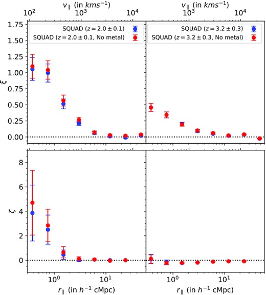
Effect of metal contamination on absorber-based longitudinal two- and three-point correlation (top to bottom) of Lyα absorbers (NH i > 1013.5 cm−2) as a function of longitudinal scale for different redshift intervals. Measurements with and without metal line contamination are shown in blue and red points, respectively. The error bars shown correspond to the larger of the two errors: one-sided Poissonian uncertainty in the number of absorber pairs (or triplets) corresponding to ±1σ or bootstrapping error.
6 EFFECT OF VARIOUS PARAMETERS ON THE CLUSTERING OF Lyα ABSORBERS
In this section, we investigate the effect of peculiar velocity and astrophysical parameters of the IGM on the clustering properties of Lyα absorbers using simulation box at |$z$| = 2. First, we check the effect of peculiar velocities using spectra generated by switching off the velocity field (other than thermal and natural broadening) while generating the spectrum. Next we check how changing the UVB changes clustering by simply varying the ΓH i parameter during the simulated flux generation stage. We will then study the effect of the thermal state and thermal history of the IGM using the two simulation boxes mentioned in Section 3: the ‘fiducial’ box with Khaire & Srianand (2019) UVB (i.e. α = 1.8) and the ‘hot’ box with ‘enhanced α = 1.8’ UVB. We will also investigate the impact of wind and AGN feedback on the clustering signal using Sherwood simulations.
6.1 Effect of peculiar velocities
We check the effect of peculiar velocities on the clustering of Lyα absorbers using our fiducial simulation box. We turn-off the peculiar velocities of the SPH particles in our simulation during the forward modelling process and generate simulated spectra. We compute the two- and three-point correlation of the Lyα absorbers obtained by Voigt profile fitting of these spectra. We then compare this two- and three-point correlations obtained with the ones computed with peculiar velocities turned on. The results are plotted in Fig. 9. In case of two-point correlation, we find that correlation amplitude is amplified at all scales greater than 0.25 h−1 cMpc when the peculiar velocity is turned on. The amplification is strongest at r∥ = 0.5–1 h−1 cMpc where peculiar velocity increases the correlation amplitude by a factor of ∼3. The amplification becomes weaker at larger scales with an amplification of only ∼1.2 at r∥ = 2–4 h−1 cMpc. It is also evident from the figure that the radial profile of ξ(r) is steepened appreciably by the presence of peculiar velocity. The ξ(r) obtained when the peculiar velocity is off is still steeper than ξ(r) profile seen along the transverse direction in our simulations (see fig. 7 of Maitra et al. 2020a). It will be interesting to see whether such a trend is also seen in observed transverse correlations. Simultaneous measurement of transverse and longitudinal correlations will allow us to probe the parameters of the background cosmology (the so-called Alcock–Paczyński test; Alcock & Paczynski 1979).
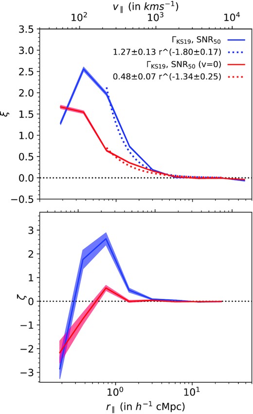
Effect of peculiar velocity on two- and three-point correlation at |$z$| = 2.0. Results for models with (blue) and without (red) the effects of peculiar velocities are shown. The dashed curves in the top panel show the power-law best-fitting models for the two-point correlation at r∥ > 0.5 h−1 cMpc.
The effect of peculiar velocity is much more drastic in the case of three-point correlation. We find positive three-point correlation only at the scale of r∥ = 0.5–1 h−1 cMpc when the peculiar velocities are switched-off. At this scale, the three-point correlation is amplified by a factor of ∼5 by the presence of peculiar velocity. The trends seen here are consistent with what we found for low-|$z$| absorbers in Maitra et al. (2020b). In that case, we notice the presence of peculiar velocities increasing the two- and three-point correlations by factors of ∼1.7 and 2.1, respectively, at scales of 1–2 pMpc (|$z$| = 0.1 simulations). Thus it appears that Lyα absorbers observed over the full redshift range (i.e. 0 ≤ |$z$| ≤ 3.5) are part of converging flows. It also emphasizes the importance of accurately modelling the peculiar velocity field (i.e. redshift-space distortions) in order to measure the correct spatial clustering (and bias parameters) from the redshift-space clustering.
6.2 ΓH i dependence
By changing the ΓH i in the simulation, one effectively changes the ionization state of the IGM; a higher ΓH i results in the H i population being more photoionized and vice versa. This alters the kind of baryonic overdensities that one probes for a given NH i value. So, an absorber with a given NH i will probe higher baryonic overdensities if the IGM is more ionized. This, in turn, would mean that for absorbers with a certain minimum NH i threshold, the clustering signal would go up if one amplifies the ΓH i, since correlations would be coming from larger overdensities. With this in mind, we simulate transmitted flux with two ΓH i values: one corresponding to the upper limit of the error bar of ΓH i reported at |$z$| = 2 in Bolton & Haehnelt (2007) (Γ12 = 2.1) and the other corresponding to the lower limit of the error bar of (Γ12 = 0.8). First, we compare the NH i distribution between these two ΓH i values in the middle panel of Fig. 10. As expected, the one with larger ΓH i value is more ionized and has a lower NH i distribution.
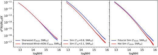
Effect of feedback process (left), H i photoionization rates (ΓH i; middle), and for thermal history (right) on the H i column density distribution function at |$z$| ∼ 2. Various simulations used are indicated in each panel.
We plot ξ, ζ, and Q as a function of longitudinal separation r∥ for these two different ΓH i values in Fig. 11. We find that the correlation amplitudes are very sensitive to ΓH i. As expected, we find that absorbers corresponding to higher ΓH i value, probing higher densities, have greater ξ and ζ values at all scales. The effect is more pronounced in the case of ζ. Interestingly, this large ΓH i effect on ξ and ζ almost nullify each other, when one considers Q. In comparison to ξ and ζ, the change in Q values does not show any coherent trend between the two ΓH i values. In summary, for a given set of cosmological parameters both two- and three-point correlation are highly sensitive to the background photoionization rates and increase with increase in ΓH i. However, in reality a well-measured NH i distribution will provide an independent constraints on ΓH i. Thus simultaneous usage of clustering (two-point correlation, three-point correlation, and Q) and NH i distribution will provide stringent constraints on ΓH i and possibly on parameters of the underlying cosmology (as clustering is also sensitive to the background cosmology).
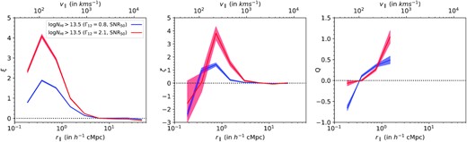
Simulated two-, three-, and reduced three-point correlation (left to right) of Lyα absorbers having NH i > 1013.5 cm−2 as a function of longitudinal separation r∥ for two different ΓH i values: one corresponding to the upper limit of the error bar of ΓH i reported at |$z$| = 2 in Bolton & Haehnelt (2007) (Γ12 = 2.1; red curves) and the other corresponding to the lower limit of the error bar of (Γ12 = 0.8; blue curves). It is evident from this figure that the clustering properties of absorbers above a given NH i threshold depend strongly on ΓH i.
6.3 Dependence on thermal and pressure broadening
Using the clustering analysis of simulated Lyα forest, Peeples et al. (2010a,b) had reported that correlations in redshift space are dominated by thermal broadening, while transverse correlations using projected quasar pair spectra are mainly dominated by pressure broadening effects. However, this analysis was based on pixel-based statistics using Lyα forest transmitted flux. Our absorber-based approach may have different dependencies on the thermal state of the IGM that we would like to explore.
As mentioned before, we base our explorations on the ‘fiducial’ and ‘hot’ models discussed in Section 3. We shoot random sightlines and calculate the correlations for the Lyα absorbers separately for the two boxes. While the thermal and pressure effects are different between the two boxes, their photoionization rates are similar. So, the correlation functions should only show the compound effect of thermal and pressure broadening between the two simulations. First, we compare the NH i distribution between these two boxes in the right-hand panel of Fig. 10. We find that there is a small difference in the distributions between the two simulations in comparison to the effect of ΓH i. The difference is more pronounced in the higher NH i end due to logarithmic scaling. This difference in the NH i distribution between the two simulations is primarily due to difference in temperature-dependent recombination rates. There can also be an additional effect of the absorbers being more thermally broadened thereby making the multiple components fitting of line-blended absorption systems more difficult (especially when we do not use higher order Lyman lines as in viper).
Next, we plot two-, three-, and reduced three-point correlation as a function of r∥ in the top panels of Fig. 12 for these two boxes. In the case of two-point correlation, there are negligible differences between the two boxes based on the observed correlation functions at scales greater than r∥ = 0.25 h−1 cMpc. In the r∥ = 0.125–0.25 h−1 cMpc bin, the amplitude of the two-point correlation is smaller for the ‘fiducial’ simulation. The three- and reduced three-point correlation are similar for the two boxes at all scales within the error bars. This similarity in the correlation functions between the ‘fiducial’ and ‘hot’ simulation is contrary to what Peeples et al. (2010a,b) had found based on a pixel-based statistics using transmitted flux. The main difference between our absorber-based approach and a flux-based approach is that in absorber-based approach, the Lyα absorbers contain information of two physical quantities: NH i and the b parameter. The b parameter is responsible for the thermal broadening seen in Lyα absorption. On the other hand, thermal broadening does not affect the measured NH i value of an absorber. So, for a fixed NH i threshold, our correlation statistics is relatively independent of the thermal broadening effect. This is not the case for flux-based approach. Since thermal broadening smooths the transmitted flux field, the flux deviation is altered in each pixel thereby altering the correlation function also. The only thermal effect we see for our absorber-based approach is at scales close to the b parameter where the inability to distinguish line blending in thermally broadened structures will slightly change the correlation amplitudes. We see this effect at scales <0.25 h−1 cMpc for the two-point correlation profile, wherein both ξ and ζ values are slightly lower for the ‘hot’ box having larger b parameter.
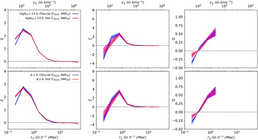
Dependence of simulated clustering on thermal parameters of the IGM. Top: two-, three-, and reduced three-point correlation (left to right) of Lyα absorbers having NH i > 1013.5 cm−2 as a function of longitudinal separation r∥ for two simulations, one with ‘fiducial’ Khaire & Srianand (2019) UVB and another with enhanced ‘hot’ Khaire & Srianand (2019) UVB. The two simulations represent the joint effect of thermal broadening and pressure broadening (from different thermal histories) on clustering. Bottom: same correlations for the two simulations, but with a constant overdensity threshold of Δ > 4. Using a constant Δ threshold nullifies any differences originating from different local thermal parameters and captures the effect of pressure broadening only from different thermal histories.
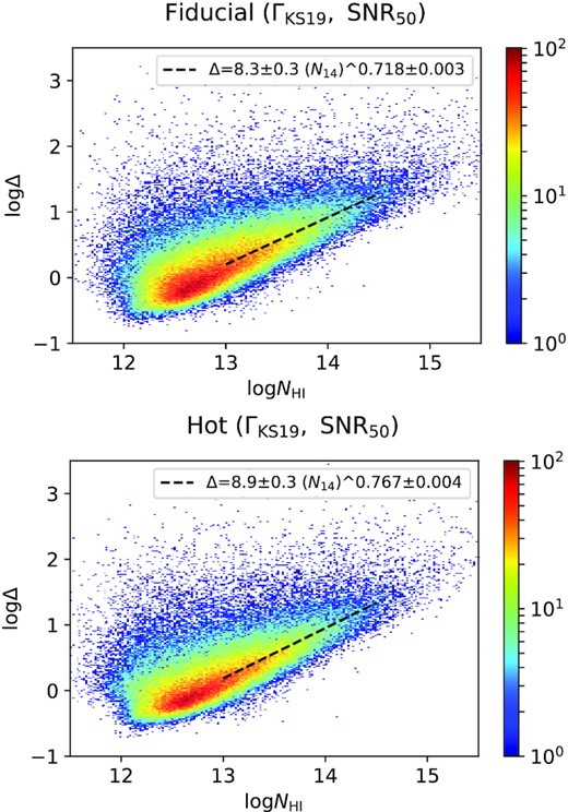
Neutral hydrogen column density (NH i) versus τ weighted baryon overdensity (Δ) plots at |$z$| = 2 for ΓH i = ΓKS19 and SNR = 50 for our ‘fiducial’ and ‘hot’ simulations. The colour represents the number of points in a certain grid. The black dashed line represents the best-fitting relationship (best-fitting values in legend) followed by the median Δ in the range of log(NH i) = (13, 14.5).
Using this, we find the NH i thresholds of the absorbers for an overdensity threshold of Δ > 4 (corresponding to logNH i > 13.56 and 13.55 for the ‘fiducial’ and ‘hot’ simulations, respectively). In the bottom panels of Fig. 12, we plot the two-, three-, and reduced three-point correlation as a function of r∥ for a constant overdensity threshold of Δ > 4. Overall, the correlations are all consistent with each other between the two simulations (as expected based on nearly identical logNH i cut-offs found for the two models). But the discrepancy in two-point correlation between the ‘fiducial’ and ‘hot’ simulations at small scales still remains. This suggests that for scales below r∥ = 0.25 h−1 cMpc the clustering is affected by the pressure broadening of the baryonic gas. So, probing clustering in Lyα absorbers at this scale will provide valuable information regarding the thermal history of the IGM. However, in order to do so, one should have a good handle on the systematics introduced by the spectral SNR and the multiple Voigt profile component decomposition of the blended absorption profile.
6.4 Dependence on feedback processes
Here we study the impact of wind and AGN feedback on the clustering properties of the Lyα absorbers at |$z$| ∼ 2 using two Sherwood simulations: one without any feedback and the other with wind+AGN feedback (for details see Section 3). As evident from the left-hand panel in Fig. 10, the two simulations are consistent in producing the number of low-NH i absorbers with each other. However, the one with feedback produces larger number of high-NH i absorbers. This effect was also pointed out by Nasir et al. (2017) in their analysis of low-|$z$| simulations (see also Gurvich, Burkhart & Bird 2017; Viel et al. 2017; Maitra et al. 2020b). Therefore, accurately measured NH i distribution at the high-NH i end can in principle constrain the effect of various feedback processes. However, one has to use simultaneous fitting of Lyα and higher series Lyman lines to have a robust deblending of the Voigt profile components at higher NH i ranges.
In Fig. 14, we plot the two-, three-, and reduced three-point correlations as a function of longitudinal separation r∥ for the Sherwood simulation with and without wind+AGN feedback. It is seen that both two- and three-point correlations are similar between the two simulations at scales greater than 0.5 h−1 cMpc. However, at scales below 0.5 h−1 cMpc, the correlation amplitudes are suppressed for the simulation with feedback. The effect is more clearly resolved in the case of two-point correlation where the error bars are much less. Interestingly, the reduced three-point correlation remains relatively unaffected at all scales. These effects are consistent with what was found for the low-|$z$| Lyα absorbers by Maitra et al. (2020b).
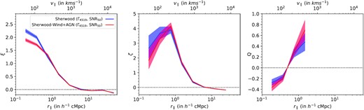
Two-, three-, and reduced three-point correlation (left to right) of Lyα absorbers having NH i > 1013.5 cm−2 as a function of longitudinal separation r∥ in Sherwood simulations with (red curves) and without wind+AGN (blue curves) feedback.
In summary, we find that both two- and three-point correlations are affected by peculiar velocities at all scales and hence, getting the correct spatial distribution requires a proper modelling of the redshift-space distortion effects. We also find that clustering in Lyα absorbers is affected by feedback processes and thermal and pressure effects at scales below 0.5 h−1 cMpc. It is, however, sensitive to H i photoionization rates at all scales. So, at scales above 0.5 h−1 cMpc, Lyα clustering can be a sensitive probe of photoionization rates for a given set of cosmological parameters.
7 REDSHIFT EVOLUTION OF CLUSTERING AND ITS IMPLICATIONS TO EVOLUTION IN THE PHYSICAL CONDITIONS OF THE IGM
In this section, we compare the measured clustering at different redshifts with the predictions of our fiducial simulation (see Section 3). Assuming the cosmological parameters used here are correct, we try to see what kind of evolution in physical state of the IGM (in particular ΓH i) is required to explain the observed trend. As shown above, the absorber-based correlation is relatively independent of thermal and pressure broadening or any feedback process at scales greater than 0.5 h−1 cMpc and is largely sensitive to ΓH i (see Section 6) for a given set of cosmological parameter. Hence our absorber-based correlation statistics should act as an independent robust probe for estimating the ionization state of the IGM.
7.1 Observed clustering and H i photoionization rates
For this exercise, we use simulated spectra from our fiducial box with Gaussian noise based on the SNR distribution from the observations (|$\rm SNR_{\rm obs}$|, see Section 3.2). We take 4000 simulated sightlines each for |$z$| = 1.7–2.3 and 2.3–2.9 bins and 1000 for |$z$| = 2.9–3.5. We consider less realizations for the high-|$z$| bin as decomposing the Lyα forest with Voigt profiles takes lot more time for the high-|$z$| case due to heavy blending of lines.
First, we use the ΓH i values from Khaire & Srianand (2019, denoted by ΓKS19) for generating the simulated sightlines. These values mainly trace the mean ΓH i measurements of Becker & Bolton (2013). In Fig. 15, we compare the two- and three-point correlations obtained from these simulations (blue curves) with the observed statistics (black points). Note that we only plot results for scales greater than 0.5 h−1 cMpc as these are mostly unaffected by thermal and pressure smoothing effects, feedback processes, or systematics involving multiple components fitting of Lyα absorption profiles. In the lowest redshift bin (i.e. 1.7 ≤ |$z$| ≤ 2.3), we find that the two- and three-point correlation from the simulations obtained with ΓKS19 agree well with the observations. This is not surprising as the ionization by the uniform UVB is valid at these redshifts and thermal parameters predicted for the Khaire & Srianand (2019) UVB model match well with the recently measured values by Gaikwad et al. (2021, see their fig. 18). Also we are using consistent cosmological parameters from the CMB experiments.
Absorber-based longitudinal two-point (top panels) and three-point correlation (bottom panels) of Lyα absorbers (NH i > 1013.5 cm−2) as a function of longitudinal scale for different redshift intervals. The error bar shown corresponds to the larger of the two errors: one-sided Poissonian uncertainty in the number of absorber pairs (or triplets) corresponding to ±1σ or bootstrapping error. The black points represent the observed correlation function obtained from joint KODIAQ+SQUAD sample. The blue curve represents correlation function obtained from gadget-3 simulation using ΓH i from Khaire & Srianand (2019). The red curve represents correlation function obtained from simulation by matching the observed mean transmitted flux.
However, for |$z$| = 2.3–2.9 bin, the predicted two- and three-point correlation amplitudes are less in comparison to the observed correlations. This deviation is even more pronounced for the |$z$| = 2.9–3.5 bin. Thus it appears that we need to produce the same range in H i column densities from relatively higher overdense regions at high redshifts. Just to explore this possibility, we next simulate spectra using ΓH i values that we get by matching the simulated mean transmitted flux with the observed mean transmitted flux (called Γobs). In this case we need to increase ΓH i by 36 per cent and 100 per cent for the redshift ranges |$z$| = 2.3–2.9 and |$z$| = 2.9–3.5, respectively. The resulting two-point correlation is also shown in Fig. 15. It is clear that if we adjust ΓH i to match the observed mean transmitted flux in our simulations the predicted clustering results have better agreement with the observations. Three-point correlation functions predicted by our models are also shown in the bottom panel of Fig. 15. Our models reproduce these measurements reasonably well.
Becker & Bolton (2013) measured ΓH i in the ranges (0.78–1.39) × 10−12 s−1, (0.65–1.16) × 10−12 s−1, and (0.60–1.11) × 10−12 s−1 for redshifts 2.4, 2.8, and 3.2, respectively. Thus our requirement that ΓH i = 1.27 × 10⁻¹² s−1 is not abnormal for the redshift bin 2.3 ≤ |$z$| ≤ 2.9. However the required ΓH i of 1.41 × 10⁻¹² s−1 for the redshift interval 2.9 ≤ |$z$| ≤ 3.5 is 2.3σ higher than the measurements of Becker & Bolton (2013). Note here we are assuming the thermal state of the gas in our simulations is correct. However, Gaikwad et al. (2021) have shown that T0 (γ) measured in the redshift range 2.5 ≤ |$z$| ≤ 3.2 are systematically higher (lower) than those predicted by the background assumed here. Also the assumption of ionization equilibrium evolution of the IGM may not be valid due to the He ii reionization at these redshifts. Especially for the highest redshift bin where one expects inhomogeneous thermal fluctuations from the end stages of He ii reionization.
In summary, we find that our clustering measurements over the redshift range 2.3 ≤ |$z$| ≤ 3.5 are not reproduced by our fiducial model. To match our observations, an absorber with a given NH i should come from regions of higher overdensity compared what has been predicted by our simulations. One possibility is to have higher ΓH i(|$z$|) compared to what has been used in our simulations. While our exercise demonstrates the need to revisit ΓH i(|$z$|) measurements, we reiterate that it has to be done by simultaneously matching various observables. As we use Voigt profile decomposed components for our clustering analysis, performing joint constraints on various parameters (like the one performed by Gaikwad et al. 2021, for constraining thermal parameters) is computationally intensive and time consuming. While that is beyond the scope of this paper, which focuses mainly on presenting the observed clustering measurements, we hope to engage in such an exercise in a near future.
7.2 Evolution of clustering in baryonic density fields
In Section 5, we studied the observed redshift evolution of clustering of Lyα absorbers for a fixed NH i threshold. This redshift evolution sources most probably from the evolution of thermal and ionization state of the IGM and the evolution in clustering of baryonic density field (see discussions in Maitra et al. 2020a). Now, instead of having a constant NH i threshold at each redshift, we vary the NH i threshold such that we will have a constant baryonic overdensity Δ threshold at all redshifts. In doing so, we would be able to study the evolution in the clustering properties of the baryonic field. This will allow us to disentangle the effects of thermal and ionization evolution of the IGM and the clustering of the baryonic density field.
For this study, we also include clustering measurements by Maitra et al. (2020b) of low-|$z$| (|$z$| < 0.48) Lyα absorbers using quasar sample of Danforth et al. (2016) observed with HST/COS. This allows us to probe the evolution in clustering of the baryonic density field measured for the Voigt profile components over a large redshift range (i.e. 0 ≤ |$z$| ≤ 3.5). First, in order to get a constant overdensity threshold at each redshift, we compute the NH i versus Δ relation from the simulations at |$z$| = 2.0, 2.6, and 3.2. In the case of |$z$| = 2.0, we will use ΓH i from Khaire & Srianand (2019) since it reproduces the observed clustering signals nicely. For |$z$| = 2.6 and 3.2, we use the ΓH i obtained by matching the observed mean flux instead, since have a better agreement with the observed clustering signals. In Fig. 16, we plot the NH i versus τ weighted Δ relationship plot at |$z=2.0, \ 2.6$|, and 3.2. The best-fitting relationship is also given in each panel. For the low-|$z$| Lyα absorbers, we take the NH i versus Δ relation from fig. 8 in Gaikwad et al. (2017a), i.e. |$\Delta =34.8\pm 5.9\times N_{14}^{0.770\pm 0.022}$|.
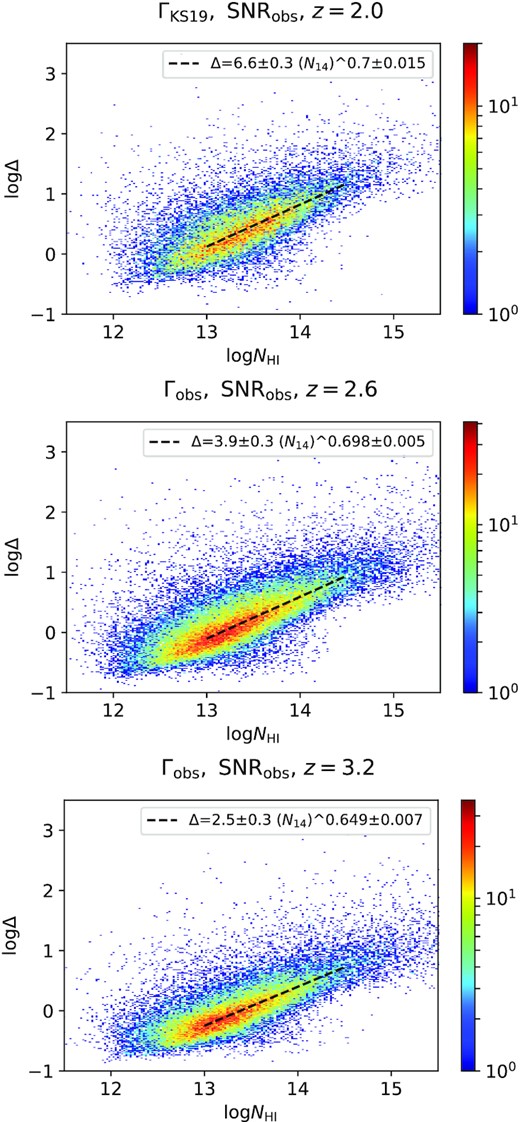
Neutral hydrogen column density (NH i) versus τ weighted baryon overdensity (Δ) plots at |$z$| = 2 for ΓH i = ΓKS19 and at |$z$| = 2.6, 3.2 with Γobs with |$\rm SNR_{obs}$| for our fiducial simulation. The colour represents the number of points in a certain grid. The black dashed line represents the best-fitting relationship (best-fitting values are provided in legend) followed by the median Δ in the range of log NH i = (13, 14.5).
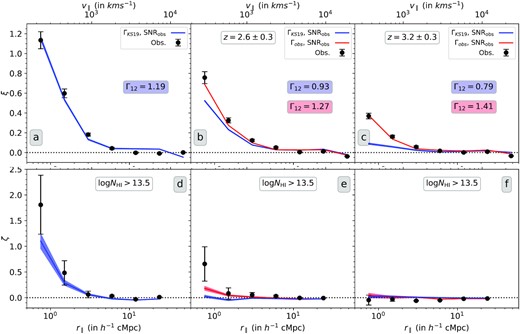
In Fig. 17, we plot the two- and three-point correlations as a function of r∥ for a constant overdensity threshold of Δ > 4 at |$z$| < 0.48, |$z$| = 1.7–2.3, |$z$| = 2.3–2.9, and |$z$| = 2.9–3.5 (corresponding to logNH i > 12.77, 13.69, 14.02, and 14.31 in the four redshift bins, respectively). We also plot simulated correlation curves for |$z$| = 2.0, 2.6, and 3.2. We provide black dotted horizontal lines for two- and three-point correlations as a perspective for the comparison of the correlation amplitudes at different redshift with respect to |$z$| = 1.7–2.3. The observed and simulated correlation functions agree reasonably well with each other, except in the r∥ = 0.5–1 h−1 cMpc bin, where the simulations produce slightly reduced correlation amplitudes. Comparing this with Fig. 15 (where the correlation amplitudes were calculated for a smaller NH i threshold of 1013.5 cm−2) indicates a somewhat weaker NH i dependence of Lyα absorbers clustering at this scale in simulations.
Absorber-based longitudinal two-, three-, and reduced three-point correlation (top to bottom) of Lyα absorbers for Δ > 4 (corresponding logNH i thresholds given) as a function of longitudinal scale for different redshift intervals. The error bar shown corresponds to the larger of the two errors: one-sided Poissonian uncertainty in the number of absorber pairs (or triplets) corresponding to ±1σ or bootstrapping error. The left-hand plot represents correlation function obtained at |$z$| < 0.48 using HST/COS sample (Danforth et al. 2016). The black points represent the observed correlation function obtained from HST/COS or joint KODIAQ+SQUAD sample. The blue and red curves represent correlation function obtained from simulation using ΓKS19 and Γobs, respectively. The black dotted horizontal lines are used as a perspective for comparing correlation amplitudes at different redshifts with respect to the 1.7 < |$z$| < 2.3 bin.
Interestingly, we also find that for a fixed Δ threshold, the redshift evolution of the correlation amplitudes is much weaker in comparison to a fixed NH i threshold. This is true for simulations too. In the case of two-point correlation, we see a weak evolution in the amplitudes at scales less than 2 h−1 cMpc in going from the highest to the lowest redshift bin. In case of three-point correlation, a slightly stronger evolution is seen in the r∥ = 1–2 h−1 cMpc bin. The significance of this is, however, less because of larger error bars at |$z$| < 0.48 and the correlations being noisy at |$z$| = 2.9–3.5. The reduced three-point correlation Q remains more or less constant within the given error bars.
This weak evolution of two- and three-point correlation seen for a fixed overdensity threshold confirms the fact that the large redshift evolution seen in the correlations for a fixed NH i threshold sources primarily from the redshift evolution of NH i versus Δ relation and does not reflect the evolution of clustering in the baryonic field itself, or the underlying dark matter probed by the Lyα absorption. This is in agreement to our findings in Maitra et al. (2020b) about the redshift evolution of transverse clustering in Lyα absorbers.
8 SUMMARY
We present measurements of LOS (i.e. redshift-space) two- and three-point correlation function of Lyα absorbers at 1.7 < |$z$| < 3.5 using the largest sample till date (i.e. 292 quasar sightlines) of high-resolution (∼6 |$\mathrm{km\, s}^{-1}$|) spectra from the publicly available KODIAQ and SQUAD samples. We report the measurements of redshift-space two-point correlation (in three redshift bins) with high significance and first detections of redshift space three-point correlation for high-|$z$| Lyα absorbers. We study their spatial profile, redshift evolution, and NH i dependence. We use hydrodynamical simulations to investigate the effects of peculiar velocities, feedback processes, the ionization state of the IGM, and thermal and pressure smoothing effects. We also compare our measurements with the predictions of simulations and draw some conclusions related to the physical state of the gas. The main results are summarized below.
8.1 Clustering properties of Lyα absorbers
We studied redshift-space two- and three-point correlation for Lyα absorbers having NH i > 1013.5 cm−2 in three redshift bins: |$z$| = 1.7–2.3, 2.3–2.9, and 2.9–3.5. We detect positive two-point correlation up to a length scale of r∥ = 8 h−1 cMpc in all the redshift bins studied with the strongest detection (>10σ) coming from the length scale r∥ = 0.25–0.5 h−1 cMpc. We also find a strong evolution of two-point correlation with redshift, which is stronger than the redshift evolution expected purely on the basis of dark matter evolution (Cristiani et al. 1997). We show that the radial profile of the two-point correlation can be well approximated with a power law for scale above 0.5 h−1 cMpc for |$z$| = 2.3–2.9 and 2.9–3.5, and above 1 h−1 cMpc for |$z$| = 1.7–2.3. The power-law index typically varies between −1.9 and −1.4 with an error of ∼0.2.
We also study redshift-space three-point correlation using triplets having equal arm length configurations. We detect positive three-point correlation up to a length scale of 2 h−1 cMpc at |$z$| = 1.7–2.3 and up to 1 h−1 cMpc at |$z$| = 2.3–2.9. We do not detect any three-point correlation at |$z$| = 2.9–3.5 for NH i > 1013.5 cm−2 absorbers (corresponding to mean overdensity at such redshifts). The strongest detection in three-point correlation is seen at 1.7 ≤ |$z$| ≤ 2.3 for scales ∼1–2 h−1 cMpc with an amplitude of 1.81 ± 0.59 (∼3.1σ significance). The corresponding reduced three-point correlation is found to be Q = 0.68 ± 0.23. Unlike three-point correlation, the reduced three-point correlation is found to be relatively scale independent.
Both two- and three-point correlation amplitudes are found to be suppressed at scales below 0.25 h−1 cMpc (∼75 |$\mathrm{km\, s}^{-1}$| at |$z$| = 2.0, ∼97 |$\mathrm{km\, s}^{-1}$| at |$z$| = 2.6, and ∼122 |$\mathrm{km\, s}^{-1}$| at |$z$| = 3.2) in all the redshift bins. This small-scale suppression can be attributed to the difficulty in identification of multiple Voigt profile components for thermally broadened absorption structure, as well as instrumental resolution and other systematic effects.
8.2 Dependence of NH i on clustering
Based on the assumption of a simple NH i versus Δ relation, one expects stronger NH i absorbers to arise from more overdense regions. It is also expected that clustering strength will scale with overdensity. With this motivation, we studied the NH i dependence of both two- and three-point correlation at scales r∥ = 0.5–1, 1–2, 2–4 h−1 cMpc in all the redshift bins. We find that both two- and three-point correlation increase with increasing NH i threshold at all scales and in all the redshift bins. Their NH i threshold dependence can be well approximated with a power law. While the two-point correlation increases with NH i threshold with a typical power-law index of ∼0.7, the three-point correlation has a stronger dependence with an index of ∼1.4. Interestingly, we find that while two- and three-point correlation increase with increasing NH i thresholds, the reduced three-point correlation Q remains relatively unaffected by it.
8.3 Effect of redshift-space distortion
Using hydrodynamical simulations at |$z$| = 2, we find that peculiar velocity amplifies the real-space two-point correlation at all scales. The effect is strongest at the scale of 0.5–1 h−1 cMpc with an amplification factor of ∼3. The effect goes weaker with increasing scale with an amplification factor of only ∼1.2 at r∥ = 2–4 h−1 cMpc. So, the peculiar velocities make the real-space two-point correlation profile steeper in redshift space. The effect of peculiar velocity is even stronger in the case of three-point correlation with an amplification factor of ∼5 at the scale of 0.5–1 h−1 cMpc. The amplification seen in two- and three-point correlations in redshift space suggests that the Lyα absorbers are part of converging flows.
8.4 Effect of astrophysical parameters
We also investigated the effect of astrophysical parameters of the IGM governed by its thermal history and ionization state, as well as the effect of feedback processes on clustering of Lyα absorbers. By comparing our ‘fiducial’ simulation with a ‘hot’ simulation, we found that thermal and pressure smoothing effects only affect the clustering signal at scales less than 0.25 h−1 cMpc. We also consider two Sherwood simulations to study the effect of wind and AGN feedback and found it to be relevant only at scales below 0.5 h−1 cMpc. The H i photoionization rate affects the clustering signals at all scales with clustering amplitude increasing with increasing ΓH i values. Hence, one can in principle use the two- and three-point correlation of Lyα absorbers at scale above 0.5 h−1 cMpc as a sensitive probe of ΓH i.
We also investigated whether simulations correctly reproduce the observed clustering statistics at scales above 0.5 h−1 cMpc using ΓH i values from Khaire & Srianand (2019) (ΓKS19). At the lowest redshift bin of |$z$| = 1.7–2.3, we find that the observed clustering statistics of Lyα forest is reproduced reasonably well by our models. However these models underpredict the clustering amplitudes at higher redshifts. We show that better matching can be found by increasing the ΓH i that will also make our simulations reproduce the observed mean transmitted flux. While this exercise demonstrates the need to revisit the ΓH i measurements, we reiterate that it has to be done by simultaneously matching various observables. We leave such a comprehensive parameter extraction to a future project.
8.5 Redshift evolution of clustering
As mentioned before, we found a strong evolution of two- and three-point correlation of Lyα absorbers having NH i > 1013.5 cm−2. In order to understand whether this corresponds to an actual evolution of clustering in the baryonic overdensities or is just a by-product of how NH i versus Δ relation evolves with redshift, we calculated the correlation with a fixed overdensity threshold of Δ > 4. We found that both two- and three-point correlations remain relatively constant in all the redshift bins. We also compared our results with the correlation statistics in |$z$| < 0.48 Lyα absorbers (Maitra et al. 2020a) and found only a slight enhancement in two- and three-point correlation signals. This confirms the fact that a strong evolution of two- and three-point correlation for a fixed NH i threshold sources from the evolution of NH i versus Δ relation.
8.6 Future perspective
We present all our clustering measurements in the tabulated form in Appendix A to enable future parameter estimation studies by other groups. As discussed before, our simulations suggested the need for a slightly elevated H i photoionization rates in comparison to the presently available measurements to match the clustering signals at higher redshifts. This necessitates a more thorough study of the entire parameter space involving thermal and ionization parameters of IGM, as well as cosmological parameters to properly constrain the H i photoionization rate. This, however, requires simultaneous Voigt profile fitting over sightlines covering the entire parameter space that is computationally expensive. This is beyond the scope of this work and is hence left as a future exercise.
The study of redshift-space clustering in Lyα absorbers at small scales (i.e. ≤0.5 cMpc) will benefit greatly from the spectra obtained using very high resolution (i.e. R ∼ 100 000) spectrographs like European Extremely Large Telescope (EELT)/HIgh REsolution Spectrograph (HIRES; Marconi et al. 2016) and Echelle SPectrograph for Rocky Exoplanets and Stable Spectroscopic Observations (ESPRESSO; Pepe et al. 2021). Both two- and three-point correlation signals at larger scales can be determined with better significance with the help of large number of high-resolution spectra from future surveys like the Maunakea Spectroscopic Explorer (MSE; McConnachie et al. 2016). Such large surveys will also pave way for the measurement of transverse three-point correlation of Lyα absorbers using projected quasar triplets. However, one needs a large number of triplet sightlines (i.e. ∼100 triplet sightlines are needed for a ∼5σ detection at scales ∼4 h−1 cMpc as discussed in section 5 of Maitra et al. 2020b) in order to obtain significant transverse three-point correlation signals. Such triplet sightlines are very rare in nature. However, with the help of future large surveys like MSE, Dark Energy Spectroscopic Instrument (DESI; DESI Collaboration et al. 2016), and Legacy Survey of Space and Time (LSST), one expects a significant improvement in the number of known quasar triplets.
In this work, we also explored the effect of metal contamination in the clustering of Lyα forest and found its effect to be negligible. It will, however, be interesting to investigate the clustering of these metal line systems and its redshift evolution by making a list of metal line system for the entire sample. Such an exercise will also allow us to perform cross-correlation studies to associate these metal line absorptions with H i absorption. Our measurement will also allow us to infer linear bias and possibly the first non-linear bias terms for the IGM at high-|$z$|. We hope to present a detailed self-consistent discussion on the bias in our upcoming work.
SUPPORTING INFORMATION
Appendix A.
Please note: Oxford University Press is not responsible for the content or functionality of any supporting materials supplied by the authors. Any queries (other than missing material) should be directed to the corresponding author for the paper.
ACKNOWLEDGEMENTS
We acknowledge the use of high performance computing facilities PERSEUS and PEGASUS at IUCAA. We thank the referee for useful comments, J. Bolton for the Sherwood simulations, and K. Subramanian, T. R. Choudhury, P. Petitjean, and A. Pranjape for useful discussions. PG acknowledges the support of the UK Science and Technology Facilities Council (STFC). The Sherwood simulations were performed using the Curie supercomputer at the Tre Grand Centre de Calcul (TGCC), and the DiRAC Data Analytic System at the University of Cambridge, operated by the University of Cambridge High Performance Computing Service on behalf of the STFC DiRAC HPC Facility (www.dirac.ac.uk). This was funded by BIS National E-infrastructure capital grant (ST/K001590/1), STFC capital grants ST/H008861/1andST/H00887X/1, and STFC DiRAC Operations grant ST/K00333X/1. DiRAC is part of the National E-Infrastructure.
DATA AVAILABILITY
The data underlying this paper are available in the paper and in its online supplementary material.
Footnotes
This configuration is equivalent to the squeezed triplet configurations (θ = 0°) with 1:2 arm length ratio.
