


ABSTRACT
A recent study suggests that the observed multiplicity of super-Earth (SE) systems is correlated with stellar overdensities: field stars in high phase-space density environments have an excess of single-planet systems compared to stars in low-density fields. This correlation is puzzling as stellar clustering is expected to influence mostly the outer part of planetary systems. Here, we examine the possibility that stellar flybys indirectly excite the mutual inclinations of initially coplanar SEs, breaking their co-transiting geometry. We propose that flybys excite the inclinations of exterior substellar companions, which then propagate the perturbation to the inner SEs. Using analytical calculations of the secular coupling between SEs and companions, together with numerical simulations of stellar encounters, we estimate the expected number of ‘effective’ flybys per planetary system that lead to the destruction of the SE co-transiting geometry. Our analytical results can be rescaled easily for various SE and companion properties (masses and semimajor axes) and stellar cluster parameters (density, velocity dispersion, and lifetime). We show that for a given SE system, there exists an optimal companion architecture that leads to the maximum number of effective flybys; this results from the trade-off between the flyby cross-section and the companion’s impact on the inner system. Subject to uncertainties in the cluster parameters, we conclude that this mechanism is inefficient if the SE system has a single exterior companion, but may play an important role in ‘SE + two companions’ systems that were born in dense stellar clusters. Whether this effect causes the observed correlation between planet multiplicity and stellar overdensities remains to be confirmed.
1 INTRODUCTION
Planets with masses/radii between Earth and Neptune, commonly called super-Earths (SEs) or mini-Neptunes, can be found around 30 per cent of solar-type stars (e.g. Lissauer et al. 2011; Fabrycky et al. 2014; Winn & Fabrycky 2015; Zhu et al. 2018). A large sample of them were discovered by the Kepler mission, with orbital periods below 300 d. SE systems contain an average of three planets (Zhu et al. 2018), generally ‘dynamically cold’, with eccentricities e ∼ 0.02 and mutual inclinations ΔI ∼ 2○ (e.g. Winn & Fabrycky 2015). However, there is an observed excess of single transiting planets that could be sign of a dynamically hot sub-population of misaligned planets (so-called Kepler dichotomy, Lissauer et al. 2011; Johansen et al. 2012; Read, Wyatt & Triaud 2017), and indicating that the mutual inclinations in a multiplanet system decrease with the number of planets (Zhu et al. 2018; He, Ford & Ragozzine 2019; Millholland et al. 2021).
Recent work by Longmore, Chevance & Kruijssen (2021) has revealed an intriguing correlation between stellar phase-space density and the architecture of planetary systems, in particular the multiplicity. This work followed a similar analysis by Winter et al. (2020), which uncovered a correlation between stellar phase-space density and the occurrence of hot Jupiters. Using Gaia DR2 data (Gaia Collaboration et al. 2018), Longmore et al. (2021) computed the local stellar phase-space density of planet-hosting stars and their neighbours (within 40 pc) to determine whether the exoplanet host was in a relatively low or high phase-space density zone compared to its neighbours. They hypothesized that stars in current stellar overdensities were previously part of dense stellar clusters, from which only local residual overdensities remain. They showed that Kepler systems in local stellar phase-space overdensities have a significantly larger single-to-multiple ratio compared to those in the low phase-space density environment. The origin of this correlation is puzzling, as stellar clustering is expected to affect mostly the outer part of planetary systems in very dense environments (Laughlin & Adams 1998; Malmberg, Davies & Heggie 2011; Parker & Quanz 2012; Cai et al. 2017; Li, Mustill & Davies 2020a). Recent works have also suggested that the correlation is weaker when using a smaller unbiased stellar sample (Adibekyan et al. 2021), and that the current stellar overdensities could be associated with stellar age or to galactic-scale ripples as opposed to dense birth clusters (Mustill, Lambrechts & Davies 2021; Kruijssen et al. 2021). Alternatively, new studies have suggested that stellar flybys can excite the eccentricities and inclinations of outer planets/companions, which then trigger the formation of hot Jupiters from cold Jupiters via high-eccentricity migration (Wang et al. 2020; Rodet, Su & Lai 2021). For this flyby scenario to be effective, certain requirements (derived analytically in Rodet et al. 2021) on the companion property (mass and semimajor axis) and the cluster property (such as stellar density and age) must be satisfied. In this paper, we will examine a similar ‘outside–in’ effect of stellar flybys on the SE systems. Earlier, Zakamska & Tremaine (2004) examined the excitation and inward propagation of eccentricity disturbances in planetary systems. Our work focuses on inclination disturbances, as they are most relevant in determining the co-transit geometry of multiplanet systems.
In recent years, long-period giant planets have been observed in an increasing number of SE systems. Statistical analysis combining radial velocity and transit observations suggests that, depending on the metallicities of their host stars, 30–60 per cent of inner SE systems have cold Jupiter companions (Zhu & Wu 2018; Bryan et al. 2019). The dynamical perturbations from external companions can excite the eccentricities and mutual inclinations of SEs, thereby influencing the observability (co-transiting geometry) and stability of the inner system (Boué & Fabrycky 2014; Carrera, Davies & Johansen 2016; Lai & Pu 2017; Huang, Petrovich & Deibert 2017; Mustill, Davies & Johansen 2017; Hansen 2017; Becker & Adams 2017; Read et al. 2017; Pu & Lai 2018; Denham et al. 2019; Pu & Lai 2020; Rodet & Lai 2021). This requires the giant planets to be dynamically hot, which can be achieved by planet-planet scattering. Alternatively, in dense stellar environments, the eccentricities and inclinations of giant planets can be increased by stellar flybys.
In this paper, we examine the possibility that SEs systems become misaligned following a stellar encounter (‘flyby-induced misalignment cascade’ scenario), using a combination of analytical calculations (for the secular planet interactions) and numerical simulations (for stellar flybys). In Section 2, we outline the proposed scenario and its key ingredients. In Section 3, we examine the inclination requirement for an outer companion to break the co-transiting geometry of two inner initially coplanar SEs. In Section 4, we evaluate the extent to which a stellar encounter can raise the inclination of an outer companion. In Section 5, we derive the expected number of ‘effective’ flybys (i.e. those that succeed in breaking the co-transiting geometry of SEs) per system as a function of the properties of the planetary system (SEs+companion) and its stellar cluster environment. Finally, in Section 6, we extend our calculation to SE systems with two outer companions. In Section 7, we examine the effect of different flyby masses. In Section 8, we summarize our main results, recalling the key figures and equations of the paper.
2 SCENARIO: FLYBY-INDUCED MISALIGNMENT CASCADE
The observed excess of single-transiting SEs or mini-Neptunes could be sign of a dynamically hot sub-population of inner (≲0.5 au) planets with appreciable mutual inclinations. The recently-evidenced correlation between single-transiting systems and stellar overdensities suggests that stellar environments could play a significant role in this misalignment. However, close-in SEs are largely protected from perturbations induced by the stellar environment thanks to their proximity to the host star.
According to recent statistical estimates, 30–60 per cent of inner SE systems have cold Jupiter companions (≳1 au, mass ≳0.3 MJ; see Zhu & Wu 2018; Bryan et al. 2020). Such companions widen the effective cross-section of the planetary system, and thus its vulnerability to the dynamical perturbations from the stellar environment. The architecture of the inner SEs can be indirectly impacted by stellar flybys through the eccentricity/inclination excitations of the outer companions.
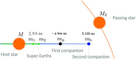
In this paper, we consider a system of two SEs with masses m1, m2 and semimajor axes a1 < a2 ≲ 0.5 au, on circular coplanar orbits around a host star (mass M = M1 ∼ 1 M⊙, radius R1 ∼ 1 R⊙). An outer companion (mass mp ≪ M) is located at ap on an initially circular coplanar orbit (see Fig. 1). In Section 6, we will consider the case of two exterior companions surrounding SEs.
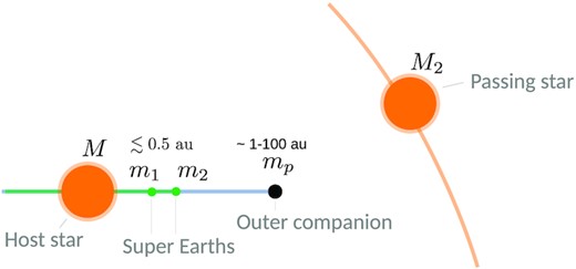
Schematic of the flyby-induced misalignment cascade scenario. An initially coplanar system comprising two inner planets (SEs) and an outer companion encounters a passing star. The stellar flyby changes the orbital inclination of mp, which then induces misalignment between the orbits of m1 and m2.
The system may experience close encounters with other stars, if the stellar density is large enough. This is typically the case in the beginning of the planetary system’s life, when it is embedded in its dense birth cluster. Most of these clusters are loosely bound or unbound, so that they tend to be disrupted over tens of millions of years (the current phase-space overdensities would be the remnants of these clusters). However, in the early phase of the cluster, close encounters may be frequent enough to influence the planetary architecture.
In the following sections, we will derive the minimum required inclination of the companion Ip,crit to break the SEs co-transiting geometry, and the corresponding likelihood that a stellar encounter would generate such an inclination.
3 SECULAR DYNAMICS OF PLANET MISALIGNMENT
When the outer companion planet to the SEs in an initially coplanar system suddenly becomes misaligned by Ip, the mutual inclination ΔI between the SEs will oscillate around a forced value (Lai & Pu 2017; Rodet & Lai 2021). In the following, we derive the minimum misalignment Ip,crit required for the forced inclination to be greater than the critical value ΔIcrit (see equation 1). In theory however, due to the oscillation of ΔI, the co-transiting geometry of the SEs will be broken only part of the time even if the forced inclination is greater than ΔIcrit.
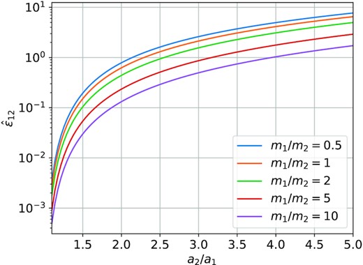
The rescaled coupling parameter |$\hat{\varepsilon }_{12}$| as a function of the semimajor axial ratio a2/a1 of the SE system, for different mass ratios m1/m2 (see equation 8). Systems with higher |$\hat{\varepsilon }_{12}$| are more easily perturbed by the outer companion.
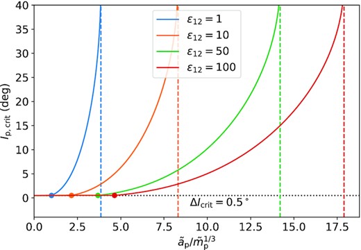
Minimum companion’s inclination Ip,crit required to produce a forced misalignment ΔIcrit = 0.5○ between two SEs (equations 12 and 14), as a function of the scaled companion semimajor axis, |$\tilde{a}_{\rm p}/\tilde{m}_{\rm p}^{1/3} = a_{\rm p}/(1~\mathrm{au}) ~ (m_{\rm p}/\mathrm{M_{J}})^{-1/3}$|, for different inner SEs systems, characterized by different values of ε12 (see equation 7). The horizontal dashed line indicates ΔIcrit = 0.5○, the filled circles indicate the change of regimes (between ε12,p > 1 and ε12,p < 1), while the vertical dashed lines indicate the maximum |$\tilde{a}_{\rm p}/\tilde{m}_{\rm p}^{1/3}$|, beyond which it is impossible to generate ΔIcrit = 0.5○ regardless of the Ip value (see equation 15).
4 EFFECT OF FLYBY ON THE OUTER PLANET
In this section, we calculate the expected effect of a stellar flyby on the orbit of the outer planet/companion, and estimate the likelihood that the companion can attain Ip > Ip,crit. To this end, we perform a suite of N-body simulations to determine the distribution of the post-flyby inclination Ip and eccentricity ep. Following a similar approach to Rodet et al. (2021), we suppose that the companion (with mp ≪ M2, the mass of the flyby star) is on an initially circular orbit, and we ignore the inner planets (their proximity to the host star effectively shields them from stellar encounter). We integrate a nearly parabolic (e = 1.1) encounter between two equal-mass stars using IAS15 from the Rebound package. The integration time is chosen so that the distance between M1 and M2 is equal to 100ap at the beginning and end of each simulation, and the time-step is adaptive. We sample uniformly the dimensionless distance at closest approach |$\tilde{q} \equiv q/a_{\rm p}$| (where q is the periastron of the encounter) from 0.05 to 10, the cosine of the inclination cos i, and the argument of periastron ω of the flyby, and the initial phase λp of the planet mp. For each |$\tilde{q}$|, we carry out 30 × 20 × 20 (in cos i, ω, λp) = 12 000 simulations, and obtain the final orbital elements of the planet. The effect of the flyby on Ip is mainly determined by the flyby inclination i, so we interpolate our data using the 30 tested inclinations to produce a denser grid of results (see Fig. A1) and avoid under-sampling effects in computing the Ip distribution (see below).
4.1 Effect on the inclination
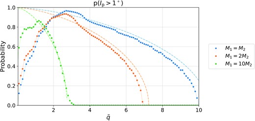
For a given |$\tilde{q}$|, we derive p(ep < 1), the probability that the planet remains bound, and p(Ip > Ip,min), the probability that the planet remains bound and has a final inclination larger than some specified Ip,min. These probabilities are shown in Fig. 4 as a function of |$\tilde{q}$|, for different values of Ip,min. For |$\tilde{q}\gtrsim 3$|, p(Ip > Ip,min) can be derived analytically using the secular approach. This derivation is detailed in the Appendix, as well as the comparison with the N-body results.
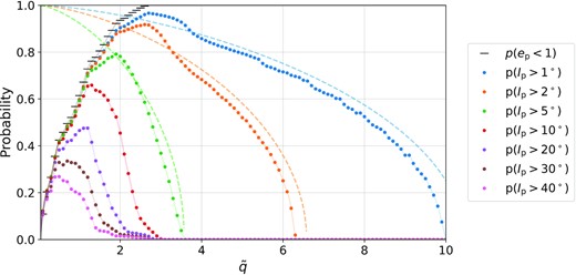
The probability p(Ip > Ip,min) for a flyby to raise the inclination of the outer planet to Ip > Ip,min (while keeping the planet bound), as a function of the dimensionless distance at closest approach |$\tilde{q} = q/a_{\rm p}$|. Each point is computed from 30 × 20 × 20 N-body simulations that sample the flyby geometry. The dashed lines are the analytical results in the secular approximation, assuming a parabolic encounter (see the Appendix for derivation and comparison). The difference between the approximation and the simulations is due in part to the N-body set-up, where the eccentricity of the flyby is 1.1 rather than 1. The short bars give p(ep > 1), the probability that the planet remains bound after the flyby.

4.2 Effect on the eccentricity
Stellar flybys not only change the inclination of the outer planet but also excite the planet’s eccentricity. Fig. 6 shows the joint distribution of Ip and ep after stellar flybys. The inclination increases are correlated to eccentricity excitations, so that the post-flyby orbit of the planet is not circular. However, its eccentricity will very likely stay low (ep ≲ 0.5) if the inclination gain is small (Ip ≲ 5○). In this case, the inclination dynamics presented in Section 3 is largely unchanged compared to the circular orbit case. When we consider higher Ip, then the eccentricity can become larger. In that case, the stability of the system is not guaranteed, so the inclination dynamics for circular orbit may not hold. In the following section, we will show that the occurrence rate of our flyby-induced misalignment scenario depends mostly on the statistics for small Ip, so that we can safely ignore the eccentricity’s effect on the inclination dynamics. In particular, we can neglect the cases where the flyby induces strong scatterings between planets.
Correlation between the eccentricity ep and inclination Ip of the outer planet after stellar flybys. The plots are generated from N-body simulations with different flyby geometries and distance at closest approaches, and the colour scales logarithmically with the local density of simulations. The plots only show simulations where the planet remains bound. The upper panels gather all flyby distances at closest approach |$\tilde{q}$| (with the right-hand panel showing a zoom-in on the low inclination part of the left-hand panel), the lower panels distinguish three different ranges of |$\tilde{q}$|. The stripes-like structure in the lower right-hand panel is not physical, and is due to the discrete inclination sampling.
5 OCCURRENCE RATE OF SUPER-EARTH MISALIGNMENT INDUCED BY STELLAR FLYBYS: SINGLE OUTER PLANET
Figs 7 and 8 show |$\mathcal {N}(\Delta I \gt 0.5^\circ , a_{\rm p})$| as a function of the semimajor axis of the outer planet ap, for different values of mp and ε12 [which characterizes the coupling of the inner SE system, see equation (7)]. The two regimes (linear and decreasing power-law dependence of ap) are clearly visible on the plots. Moreover, there is a maximum ap,max above which no Ip can induce the required ΔIcrit (see equation 15), and thus |$\mathcal {N}(\Delta I\gt \Delta I_{\rm crit}, a_{\rm p}) = 0$| for ap > ap,max.
![Number of stellar flybys that generate ΔI > ΔIcrit = 0.5○ in the SE system as a function of ap of the outer planet companion, for different values of mp [solid lines; see equations (20)–(22)]. Each curve terminates at ap,max, given by equation (15). The peak of each curve is located at $(a_{\rm p, peak}, \mathcal {N}_{\rm max})$. The inner SE system is characterized by ε12 = 10 (equation 7), and the cluster parameters are fixed to the fiducial values of equation (17): tcluster = 20 Myr, σ⋆ = 1 km.s−1, n⋆ = 103 pc−3, and $M_\mathrm{tot} = 2 \, {\rm M}_\odot$.The light dashed lines give $\mathcal {N}(I_{\rm p} \gt I_{\rm p, min}, a_{\rm p})$ for different values of Ip,min (see equation 16).](https://oup.silverchair-cdn.com/oup/backfile/Content_public/Journal/mnras/509/1/10.1093_mnras_stab3046/1/m_stab3046fig7.jpeg?Expires=1750189528&Signature=qSMivI0OCea4GtO9LHuSArCaihc8n-kDtlo3ARA9MjxHtZ0UJOAWHcc4njQxbJaDf1XksG9XqVFu4yxqwaXLgT26hrTUT9xC8NVrLOIE-xwAhMlUkDVyZ42IxwVz1fm5V13JS0WUPTo3oCBnBLNfkAk~i7N5kX7VC4AgzSJvXnFER4AatUKGDTQa9DdRN~1MzYcKH2Y-4OYea4MnjqHxp42-ILDgyvghM1E4YfYCPMgIXR9nvf8Ktka2PaJlx3sJ86j1BKAuj1rW-a~mUN3pkPJAIVsj9f0Zpackrppv8VyqrOlM7z4qdWygZ3yqal6GGDIwz8zGoCwcrRUNVlDkAg__&Key-Pair-Id=APKAIE5G5CRDK6RD3PGA)
Number of stellar flybys that generate ΔI > ΔIcrit = 0.5○ in the SE system as a function of ap of the outer planet companion, for different values of mp [solid lines; see equations (20)–(22)]. Each curve terminates at ap,max, given by equation (15). The peak of each curve is located at |$(a_{\rm p, peak}, \mathcal {N}_{\rm max})$|. The inner SE system is characterized by ε12 = 10 (equation 7), and the cluster parameters are fixed to the fiducial values of equation (17): tcluster = 20 Myr, σ⋆ = 1 km.s−1, n⋆ = 103 pc−3, and |$M_\mathrm{tot} = 2 \, {\rm M}_\odot$|.The light dashed lines give |$\mathcal {N}(I_{\rm p} \gt I_{\rm p, min}, a_{\rm p})$| for different values of Ip,min (see equation 16).

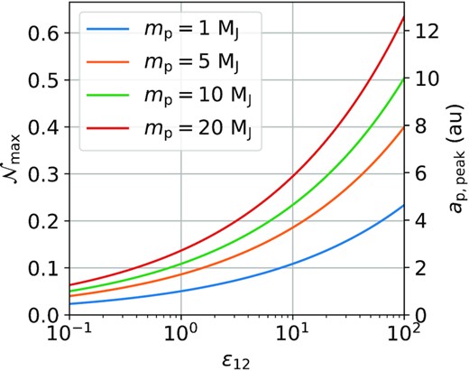
The maximum possible number of flybys |$\mathcal {N}_{\rm max}$| that can produce ΔI > 0.5○ in the SE system and corresponding ap,peak as a function of ε12, for different mp (see equations 23–24). The |$\mathcal {N}_{\rm max}$| value uses the cluster parameters tcluster = 20 Myr, σ⋆ = 1 km s−1, and n⋆ = 103 pc−3. |$\mathcal {N}_{\rm max}$| scales with |$m_{\rm p}^{1/3}$|, but can be easily rescaled for different parameters (see equation 17) and different mp (since |$\mathcal {N}_\mathrm{max} \propto m_{\rm p}^{1/3}$|).
6 SUPER-EARTH SYSTEMS WITH TWO EXTERIOR COMPANIONS
In the previous section, we have seen that flyby-induced misalignment of SEs by way of a single outer companion/planet is somewhat inefficient (see equation 24). In this section, we add a second companion mb in a circular orbit (semimajor axis ab) around the host star (see Fig. 10). This second companion can be farther away, thus increasing the effect cross-section for flybys. The flyby-induced misalignment Ib on this second companion will misalign the first companion by Ip, which will then increase the mutual inclination ΔI between the SEs.
Schematic of the flyby-induced misalignment cascade scenario considered in Section 6: an initially coplanar system comprising two inner planets (SEs) and two outer companions encounters a passing star.
Similarly to Section 5, we focus on the cases where the architecture of the system pre-flyby is coplanar. For companions at large separations (≳50 au, Tokovinin 2017), this is not the most likely configuration. If a wide companion form with a primordial inclination, then flybys are not needed to misalign the inner system. In such systems, the stellar environment is expected to play a less important role than the initial conditions in the inner system dynamics. Here, we are interested in systems that are significantly impacted by the stellar environment, so we focus on initially coplanar companions.
ε12,p ≳ 1 and |$\varepsilon _{\rm \bar{12}p, b} \gtrsim 1$|
The first companion mp has a strong influence on the SEs, and the second companion mb has a strong influence on the inner ‘SEs+mp’ system. The misalignment Ib of mb generated by a flyby is then directly transmitted to mp and the SEs (i.e. ΔI ≃ Ip ≃ Ib).
ε12,p ≲ 1 and |$\varepsilon _{\rm \bar{12}p, b} \gtrsim 1$|
The first companion has a weak influence on the SEs, but the second companion has a strong influence on the inner system. The misalignment of mb is directly transmitted to mp (i.e. Ip ≃ Ib), but the mutual inclination ΔI of the SEs is reduced from Ip (see equation 9).
ε12,p ≳ 1 and |$\varepsilon _{\rm \bar{12}p, b} \lesssim 1$|
The first companion has a strong influence on the SEs, but the second companion has a weak influence on the inner system. The misalignment Ip of mp is then reduced from Ib, while it is directly transmitted to the SEs (i.e. ΔI ≃ Ip).
ε12,p ≲ 1 and |$\varepsilon _{\rm \bar{12}p, b} \lesssim 1$|
The first companion has a weak influence on the SEs, and the second companion also has a weak influence on the inner system. The misalignment of mp is then reduced from Ib, and the mutual inclination of the SEs is also reduced from Ip.
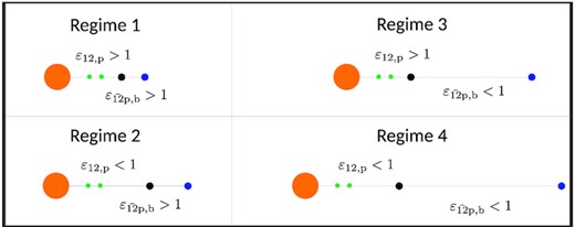
Schematic of the four different regimes characterized by the coupling parameters ε12,p (see equation 6) and |$\varepsilon _{\rm \bar{12}p, b}$| (see equation 29). When ε12,p ≳ 1 (≲1), the first companion mp has a stronger (weaker) influence on the SEs (m1 and m2) compared to the mutual coupling between m1 and m2; when |$\varepsilon _{\rm \bar{12}p, b} \gtrsim 1$| (≲1), the second companion mb has a stronger (weaker) influence on the inner ‘SEs+mp’ system compared to the mutual coupling between the SEs and mp. In this schematic, a companion is strong if its distance to the inner bodies is similar to the distance between the inner bodies or if it is much more massive.
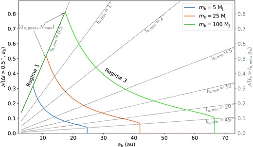
Number of stellar flybys that generate ΔI ≳ ΔIcrit = 0.5○ in the SE system as a function of ab of the outermost companion, for different values of mb (solid lines; see equation 35). Each curve terminates at ab,max, given by equation (34). The inner SE system is characterized by ε12 = 10 (equation 7), |$a_{\bar{12}} = 0.5$| au, and the inner companion’s parameters are fixed to ap = 2 au and mp = 1 MJ, so that ε12,p ≳ 1. This situation corresponds to regimes 1 (for small ab) and 3 (for high ab). The cluster parameters are fixed to the fiducial values of equation (17): tcluster = 20 Myr, σ⋆ = 1 km s−1, and n⋆ = 103 pc−3. The light dashed lines give |$\mathcal {N}(I_{\rm b} \gt I_{\rm b, min}, a_{\rm b})$| for different values of Ib,min (see equation 16, applied to the outermost companion). See Figs 7 and 8 for the cases of SEs with a single companion.
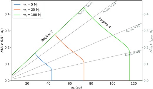
Same as Fig. 12, except for ap = 5 au, corresponding to ε12,p = 0.07 (see equation 7). For this value of the coupling parameter, the first companion mp should have a minimum Ip,crit ∼ 7○ > ΔIcrit (see equation 14) to generate a misalignment ΔI > ΔIcrit within the inner SE system. This case corresponds to regimes 2 (for small ab) and 4 (for high ab).
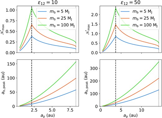
Maximum number of flybys |$\mathcal {N}_{\rm max}$| that gives ΔI ≳ ΔIcrit = 0.5○ (top) and optimal ab,peak (bottom) as a function of ap (equation 37), for different values of mb. Note that ab,peak is chosen so as to maximize the number of flybys, i.e. such that |$\varepsilon _{\rm \bar{12}p,b} = 1$| (equation 36). The optimal ap is indicated with a dashed vertical line: it corresponds to ε12,p = 1 and does not depend on mb. The maximum ap at around 8 au (left) or 15 au (right) is similarly independent of mb (equation 15). The SEs system is fixed, with ε12 = 10 (left) and ε12 = 50 (right), |$a_{\bar{12}} = 0.5$| au, and the mass of the first companion is fixed to mp = 1 MJ. The cluster parameters are tcluster = 20 Myr, σ⋆ = 1 km s−1 , and n⋆ = 103 pc−3. Note that |$\mathcal {N}_{\rm max}$| scales with |$a_{\bar{12}}^{-1/2}$| and |$m_{\rm p}^{-1/3}$|, and is proportional to tcluster, |$\sigma _\star ^{-1}$|, and n⋆.

Maximal ‘peak’ number of flybys |$\mathcal {N}_{\rm max,peak}$| that gives ΔI ≳ ΔIcrit = 0.5○ (top) and corresponding ab,peak (bottom) as a function of ε12 (equations 41–42), for different values of mb. The optimal ap and ab values, ap,peak and ab,peak, are set by ε12p = 1 and |$\varepsilon _{\rm \bar{12}p,b} = 1$| (equations 38–39), so as to maximize the number of flybys. The optimal ap,peak is indicated with a dashed black line on the bottom plot – it does not depend on mb. The SEs location is set to |$a_{\bar{12}} = 0.5$| au, and the mass of the first companion is fixed to mp = 1 MJ. The cluster properties are tcluster = 20 Myr, σ⋆ = 1 km s−1, and n⋆ = 103 pc−3, but note that |$\mathcal {N}_{\rm max, peak}$| scales with |$a_{\bar{12}}^{-1/2}$| and |$m_{\rm p}^{1/6}$|, and is proportional to tcluster, |$\sigma _\star ^{-1}$|, and n⋆.
7 DEPENDENCE ON THE MASS OF THE STELLAR PERTURBER
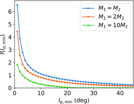
Our calculations in the previous sections assume that the stellar perturber has the same mass as the host star of our planetary system (M1 = M2). In reality, most of the stars in the Galaxy are less massive than |$1\, {\rm M}_\odot$|, and the impact of a flyby depends on the mass of the perturber M2. On the other hand, for a fixed stellar mass density, if the mass is mostly distributed between lighter stars, we expect n⋆ to be higher.
Similar than Fig. 4, for Ip,min = 1○ and different M2 (equation 43). For the same distance at closest approach, the effect of the flyby decreases with decreasing perturber mass M2. For small |$\tilde{q}$|, a decreased mass leads to less configurations becoming unbound, which ultimately increases the probability to have a bound system with small inclination.
8 SUMMARY AND DISCUSSION
8.1 Summary
In this paper, we have studied a new mechanism for dynamical excitations of Super-Earths (SE) systems following a close stellar encounter. We are motivated by the recently claimed correlation between the multiplicity observed in Kepler transiting systems and stellar overdensities (Longmore et al. 2021). The proposed mechanism consists of stellar flybys exciting the inclinations of one or two exterior companion giant planets (or brown dwarfs), which would then induce misalignment in an initially coplanar SE system. Even a modest misalignment (ΔI ≳ 0.5○) could break the co-transiting geometry of the SEs, resulting in an apparent excess of single-transiting systems. We study two cases: in one, the SE system has a cold Jupiter companion at a few au; in the other, the SE system has two companions, a cold Jupiter and a wider planetary or substellar companion. Our results can be rescaled easily with the SE system or companion properties.
To evaluate the probability for a system to experience such an ‘effective’ flyby (that can generate ΔI ≳ 0.5○ for the SEs), we combine analytical calculation (on stellar encounters and the secular coupling between the SEs and companions) with N-body simulations (to evaluate the effects of representative close encounters). Given the large parameter space and related uncertainties, we have attempted to present our results in an analytical or semi-analytical way, so that they can be rescaled easily for different SE and companion properties and stellar cluster parameters.
When the SE system only has one planetary companion, we show that the mechanism is relatively ineffective. If the outer planet is close to the SEs, then stellar flybys will have a small chance of changing its orbital inclination. On the other hand, if the outer planet is farther away, then it will have little impact on the SE dynamics, and on their transiting geometry in particular. This trade-off is shown in Figs 7 and 8. For given density, velocity dispersion, and lifetime of the stellar cluster, we can evaluate the expected number of stellar flybys that will disrupt the co-transiting geometry of the SEs as a function of the SE system (characterized by the coupling parameter ε12, equation 7) and the companion properties (semimajor axis and mass). Fixing all parameters but the companion semimajor axis (ap), the number of ‘effective’ flybys peaks for an optimal ap which, for typical Kepler SEs, corresponds to a few astronomical units for mp ∼ 1 MJ (see equation 23). The corresponding maximum number of effective flybys and its dependencies in all related parameters is displayed in equation (24). With only one companion, this flyby-induced misalignment scenario is unlikely to produce statistically significant effect of the SE multiplicity; even when assuming a high cluster density, less than 1 in 10 suitable systems (with an exterior giant planet) will experience the required stellar flyby.
When the SE system has two companions, the effective cross-section for stellar flybys increases. The misalignment induced on the outermost (second) companion mb by the flyby can be transmitted to the inner (first) companion mp, which would them be able to break the co-transiting geometry of the SEs. A relatively close (small ab) second companion would have a strong influence on the inner system (SEs and mp) (characterized by the parameter |$\varepsilon _{\rm \bar{12}p, b}$|, equation 29), and transmit its misalignment Ib fully to the first companion (i.e. Ib ∼ Ip for |$\varepsilon _{\rm \bar{12}p, b} \gtrsim 1$|). On the other hand, a far-out second companion has a better chance of experiencing close stellar flybys, but could have a smaller effect on the inner system. The trade-off is shown in Figs 12 and 13 for two different locations of the first companion, close to the SEs or farther away. Fixing the properties of the SEs, the number of effective flybys peaks for an optimal combination of ap and ab which, for typical Kepler ‘SE+cold Jupiter systems’, corresponds to a few AU and tens of AU, respectively, for substellar second companions. The corresponding number of flybys and its dependencies on various parameters is displayed in equation (41). The optimal architecture (semimajor axes of the two companions as a function of their masses and the SE parameters) is described in equations (38) and (39) (see Figs 14 and 15). Our calculations show that the number of effective flybys (that can generate ΔI > 0.5○ for the SEs) increases significantly when a second companion is added, suggesting that most initially coplanar SE systems with two companions in stellar overdensities will experience a flyby that will misalign their orbits, and thus break the co-transiting geometry.
8.2 Discussion
In this paper, we have adopted some simplifications in deriving the analytical estimates of the effect of flybys on SE systems with exterior companions. One of the simplifications that we made was to ignore the encounters with binary stars. Tight binaries with separation abinary ≪ ap are expected to behave similarly to a single stellar perturber. On the other hand, only one component will play a role in encounters with large-separation binaries (abinary ≫ ap). For intermediate cases, more exploration is needed (see e.g. Li, Mustill & Davies 2020b).
Our calculations show that SE systems with only one outer companion are unlikely to be much impacted by the stellar flybys, while systems with two companions are likely to be impacted (depending on various parameters). However, SE systems with two companions may be rarer than their one-companion counterparts. Ultimately, further information on the correlation between inner SE systems and exterior planets/substellar companions will be needed to determine the relative prevalence of the mechanisms studied in this paper. Moreover, a deeper knowledge on the properties of stellar birth clusters (lifetime and density in particular) and their relation to the observed overdensities characterized in Winter et al. (2020) and Longmore et al. (2021) is needed to draw firm conclusions on the role of the flyby-induced misalignment scenario in multiplanet systems.
ACKNOWLEDGEMENTS
We thank the referee, A. Mustill, for useful comments that have improved this paper. This work has been supported in part by the NSF grant AST-17152 and NASA grant 80NSSC19K0444. We made use of the python libraries numpy (Harris et al. 2020), scipy (Virtanen et al. 2020), and pyqt-fit, and the figures were made with matplotlib (Hunter 2007).
DATA AVAILABILITY
The output of the N-body flyby simulations (Section 4) can be found on https://github.com/LaRodet/FlybySimulations.git. All the figures can be directly reproduced from this data set and from the equations.
REFERENCES
APPENDIX: SECULAR PERTURBATION ON THE INCLINATION BY A PARABOLIC FLYBY
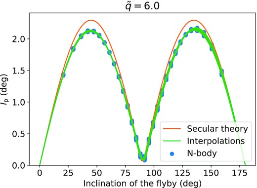
Inclination of the planet after the flyby, from the secular theory (orange, equation A4) and N-body simulations (clustered blue dots). Each of the 30 simulated inclinations groups 20 × 20 simulations, with various ω and λp. The green lines are the interpolation of Ip over the inclination of the flyby for each couple (ω, λp). These results and interpolations are used to produce Fig. 4.
