


ABSTRACT
We have carried out relativistic three-dimensional simulations of high-power radio sources propagating i,nto asymmetric cluster environments. We offset the environment by 0 or 1 core radii (equal to 144 kpc), and incline the jets by 0, 15, or 45° away from the environment centre. The different environment encountered by each radio lobe provides a unique opportunity to study the effect of environment on otherwise identical jets. We find that the jets become unstable towards the end of the simulations, even with a Lorentz factor of 5; they nevertheless develop typical Fanaroff–Riley class II radio morphology. The jets propagating into denser environments have consistently shorter lobe lengths and brighter hotspots, while the axial ratio of the two lobes is similar. We reproduce the recently reported observational anticorrelation between lobe length asymmetry and environment asymmetry, corroborating the notion that observed large-scale radio lobe asymmetry can be driven by differences in the underlying environment.
1 INTRODUCTION
Radio sources are inextricably linked to their host galaxy through feedback processes (McNamara & Nulsen 2007; Fabian 2012; Hardcastle & Croston 2020) that influence black hole growth (Rafferty et al. 2006; Alexander & Hickox 2012; Dubois et al. 2012), star formation (Gaibler et al. 2012; Weinberger et al. 2018), and the small- to large-scale environment through gas circulation, heating, and shock driving (Croton et al. 2006; Rafferty, McNamara & Nulsen 2008; Mukherjee et al. 2016; English, Hardcastle & Krause 2016; Yates, Shabala & Krause 2018). Their influence on galaxy evolution and formation is underscored by the significant attention paid towards analytic (Scheuer 1974; Begelman & Cioffi 1989; Falle 1991; Kaiser & Alexander 1997; Alexander 2002, 2006; Shabala & Alexander 2009; Krause et al. 2012; Raouf et al. 2017), semi-analytic (Turner & Shabala 2015; Hardcastle 2018; Raouf et al. 2019), and numerical (Krause 2005; Gaibler, Khochfar & Krause 2011; Wagner, Bicknell & Umemura 2012; Hardcastle & Krause 2014; Mukherjee et al. 2016; Bicknell et al. 2018; Yates et al. 2018; Li et al. 2018; Perucho, Martí & Quilis 2019; Horton, Krause & Hardcastle 2020b) models to understand this phenomenon. These radio sources are most commonly studied through observations of the kpc to Mpc scale radio lobes (Bennett & Simth 1962; Hardcastle et al. 2019b; Seymour et al. 2020) inflated by the relativistic jet beam, throughout which a population of relativistic electrons accelerated at shocks emits through synchrotron and inverse-Compton processes (Kaiser, Dennett-Thorpe & Alexander 1997; Turner et al. 2018a)
Radio sources have historically been classified into two distinct categories (Fanaroff & Riley 1974) based on whether the large-scale lobe morphology is edge-darkened (Fanaroff–Riley class I, FR I) or edge-brightened (FR II). As radio telescope sensitivity and resolution have increased, this distinction has become increasingly murky: compact radio sources with some low-frequency extended emission have been termed FR 0s (Baldi, Capetti & Giovannini 2019; Capetti et al. 2019; Garofalo & Singh 2019); low luminosity (|$L_{150} \le 10^{25}\, \textrm {W~Hz}^{-1}$|) FR II radio sources have been observed (Mingo et al. 2019); radio sources that exhibit hybrid FR I/II characteristics suggest that precession and projection effects can drastically alter the observed morphology (Krause et al. 2019; Harwood, Vernstrom & Stroe 2020; Horton et al. 2020a, b); the consideration of mergers, cluster weather, and remnant or restarting radio sources further complicates the observed lobe morphology (Mahatma et al. 2018; Yates et al. 2018; English, Hardcastle & Krause 2019; Hardcastle et al. 2019a; Joshi et al. 2019; O’Neill et al. 2019; Bruni et al. 2020).
Many complex processes are likely at work behind the observed morphologies; however, one key factor is the environment into which the radio source is expanding. Analytic models predict a strong dependence on lobe size as a function of environment (Kaiser & Alexander 1997; Alexander 2006; Krause et al. 2012), which is reproduced by simulations (Mendygral, Jones & Dolag 2012; Hardcastle & Krause 2013; Bourne & Sijacki 2017; Yates et al. 2018). Observationally, the observed length asymmetry in radio lobes pairs was recently shown to be linked to the underlying environment asymmetry, as traced by optical galaxy counts by Rodman et al. (2019), who found a statistically significant anticorrelation between the two.
At first sight, it might sound trivial that jets propagate more slowly into a higher density environment. However, the environment sets the pressure level in the radio lobes, which in turn affects the hydrodynamic collimation of the jet (e.g. Kaiser & Alexander 1997). Jets in a denser environment have higher pressure lobes and narrower jets that concentrate the thrust in a smaller area of the jet head and thus make it propagate faster and change the area over which feedback is distributed. While the sound speed in radio lobes is high such that, to first order, pressure differences are quickly readjusting, it is well known that dynamically changing as well as quasi-persistent pressure gradients exist, for example away from hotspots (fig. 12; Krause 2003). There is thus a non-linear feedback loop, and only a simulation that includes all these relevant processes can make a proper prediction for this situation.
In this work, we confront the findings of Rodman et al. (2019) with hydrodynamic simulations of radio jets in asymmetric environments and show that the observed radio source asymmetry is consistent with being caused by the underlying environment asymmetry. Section 2 describes the technical simulation setup, environment prescription, and parameter space explored. In Section 3 we present our findings, and our conclusions in Section 6.
Throughout this work, we adopt the Planck15 cosmology (Planck Collaboration XIII 2016) with |$H_0 = 67.6\, \textrm {km~s}^{-1}\, \textrm {Mpc}^{-1}$| and ΩM = 0.307.
2 SIMULATIONS
The simulations presented in this paper model astrophysical jets as relativistic fluid flows using the freely available numerical simulation package pluto1 (Mignone et al. 2007). We use a simulation setup that builds upon our earlier work (Yates et al. 2018), extended to model relativistic jets in three dimensions.
2.1 Environment
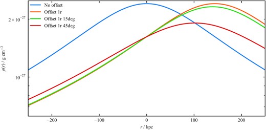
Environment density as a function of radius along the jet axis for the environment parameters described in Section 2.1. The environment centre is offset by 0 or 1 core radii, while the jet inclination angle with respect to the environment is 0, 15, or 45°.
The pressure profile is calculated from the density profile using |$P(r) = \frac{k_\textrm {B} T \rho (r)}{\mu m_\textrm {H}}$|. We take μ = 0.60 and |$T = 3.46\times 10^7\, \textrm {K}$|, consistent with observed temperatures in clusters. Cooling is not included in our simulations. This is a valid assumption provided the environment cooling time is long; the central cooling time tcool for the environment presented here is on the order of |$1.5\, \textrm {Gyr}$| for a metallicity of Z = −1.0 (Sutherland & Dopita 1993), more than an order of magnitude longer than the jet lifetimes considered in this work.
2.2 Computational methods
Version 4.3 of pluto is used to carry out the simulations presented here. The relativistic hydrodynamics physics module is used, along with the hllc Riemann solver, linear reconstruction, second-order Runge–Kutta time-stepping, the Taub–Mathews (TM) equation of state, and a Courant–Friedrichs–Lewy number of 0.33.
The simulations were carried out on a static three-dimensional Cartesian grid centred at the origin with a side length of |$l_\textrm {x,y,z} = 400\, \textrm {kpc}$|, cell count of (nx, ny, nz) = (550, 550, 960), and reflective boundary conditions. A central uniform grid patch of 100 cells is defined around the injection region in all three dimensions (|$-2.5 \rightarrow 2.5\, \textrm {kpc}$|, a resolution of |$0.05\, \textrm {kpc}$|) to ensure that injection of the initially conical jet and its hydrodynamic collimation by ambient pressure are sufficiently resolved. Either side of the central grid patch is a geometrically stretched grid consisting of 430 cells in Z, and 225 cells in X and Y; giving a minimum resolution of |$1.7\, \textrm {kpc}$| and |$2.8\, \textrm {kpc}$| per cell, respectively. Reflective boundary conditions were applied to both the lower and upper grid boundaries.
A two-dimensional spherical axisymmetric grid is used in a resolution study to verify that jet recollimation is captured correctly. In these simulations the jet is aligned with the axis of symmetry, and the simulation domain is taken to be |$(r, \theta) = (0.2\, \textrm {kpc}, 0^{\circ }) \rightarrow (800\, \textrm {kpc}, 180^{\circ })$|. A high-resolution uniform radial grid patch of 256 cells covers the injection region (|$r = 0.2 \rightarrow 2\, \textrm {kpc}$|, a resolution of |$7\, \textrm {pc}$| per cell), while the remainder of the domain is uniformly covered by 1650 cells. Azimuthally the jet injection region is uniformly resolved for each side by 300 cells over the first 5°, and 250 cells over the next 12°. A lower resolution uniform grid patch of 400 cells is placed from θ = 17° → 163°, as for the adopted jet half-opening angle of 15° this region will mainly contain sideways expansion of the jet lobe and cocoon. At a distance of |$200\, \textrm {kpc}$| this provides a resolution of |$58\, \textrm {pc}$| across the jet head. The lower radial boundary has an inflow condition within the jet nozzle; reflective boundary conditions were applied outside the jet nozzle and at the upper radial boundary. Axisymmetric boundary conditions were applied to both the lower and upper azimuthal boundaries.
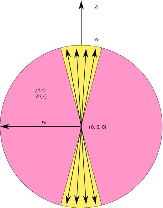
Jet injection zone.
2.3 Parameter study
We simulate a radio jet pair, each with a power of |$Q=3 \times 10^{38}\, \textrm {W}$|, typical of moderate-power FR IIs (Turner, Shabala & Krause 2018b; Shabala et al. 2020). The main science simulations consist of a pair of relativistic jets on a three-dimensional grid. We vary the offset from the cluster centre (0 or 1 core radii, corresponding to 0 or |$144\, \textrm {kpc}$|), as well as the inclination angle with respect to the centre (0°, 15°, or 45°). The jets are relativistic, γ = 5 (vj = 0.98c), have a half-opening angle θj = 10°, and are initially overpressured and underdense compared to the ambient medium. Finally, we conduct a resolution study with high-resolution two-dimensional relativistic simulations to verify that we are capturing the jet recollimation dynamics correctly in the three-dimensional simulations.
The simulations and their parameters are listed in Table 1. To aid with the discussion, in all offset cases we define the jet directed towards the cluster centre as the primary jet, while the jet directed away from the cluster centre as the secondary jet.
A list of parameters for the simulations presented in this paper. Q is the total one-sided power of the radio source, which is the same for all runs. vj is the jet velocity, roffset is the radial offset from the environment centre, θi is the inclination angle of the jet with respect to the environment centre, Θj is the temperature parameter of the jet at injection, and ηr is the relativistic generalized density contrast at injection.
| Code | Q (W) | vj (c) | roffset (kpc) | θi (°) | Θj | ηr | |
|---|---|---|---|---|---|---|---|
| Main simulations | off0r | 3 × 1038 | 0.98 | 0 | 0 | 3.2 × 10⁻³ | 5.9 × 10⁻² |
| off1r | 144 | 0 | 8.8 × 10⁻² | ||||
| off1r-15deg | 15 | ||||||
| off1r-45deg | 45 | ||||||
| 2D resolution study | 2doff0r | 0.90 | 0 | 0 | 7.5 × 10⁻⁴ | 3.7 × 10⁻¹ | |
| 2doff1r | 144 | 0 | 5.1 × 10⁻⁴ | 5.5 × 10⁻¹ |
The simulations presented here were carried out on the kunanyi (Tasmanian Partnership of Advanced Computing) and Raijin (National Computational Infrastructure) high-performance computing facilities. Between 1400 and 4800 cores were used, and the three-dimensional relativistic simulations each took approximately 300 000 CPU hours.
2.4 Synthetic radio observables
Emission due to synchrotron radiation is the main method by which the large-scale structure of radio sources can be observed. Synchrotron radiating particles are likely accelerated both along the jet and at the jet hotspots, continuing to radiate as they flow back into the radio lobes (Hardcastle et al. 2016; Matthews, Bell & Blundell 2020; Rieger & Duffy 2021). Thus to compare observed radio source structure with simulations, the synchrotron emissivity of a simulated radio source needs to be calculated. While the simulations presented here do not contain the magnetic fields necessary for a complete treatment of synchrotron radiation, the emissivity can be calculated by assuming a constant departure from equipartition for the magnetic field and electron energy densities (Kaiser et al. 1997; Turner & Shabala 2015). Magnetohydrodynamic simulations show that the ratio of particle to magnetic pressure (plasma β) remains on average constant over time (Hardcastle & Krause 2014), but has large spread spatially due to lobe turbulence (Gaibler, Krause & Camenzind 2009). Thus our assumption has the effect of smoothing out any local magnetic field variations across the lobes.
Spectral ageing is not included in this work, so the synthetic radio spectrum has an identical shape for all frequencies; frequency serves only to change the normalization j0. The emissivity is weighted by the jet tracer fluid, to account for mixing of jet and ambient material. We note that this method for calculating the emissivity does not include any losses, which alter the observed morphology of the radio source (Turner et al. 2018a) and the evolution of luminosity with time (Kaiser et al. 1997; Shabala & Godfrey 2013; Turner & Shabala 2015; Hardcastle 2018). In this work, we focus on the dynamics of the radio source, and so neglect both radiative and adiabatic losses, in addition to Doppler boosting due to relativistic fluid motions. English et al. (2016) showed that the effect of Doppler boosting on total luminosity is small due to both the small amount of emission associated with the jets and the relatively low bulk Lorentz factors found on the grid, consistent with our simulations.
3 RESULTS
3.1 Dynamics and morphology
We show logarithmic density maps of our main simulations at the end of the simulation time in Fig. 3. The jets re-collimate successfully before entraining gas later via three-dimensional instabilities and transitioning to turbulence. The jet disruption is very similar to the mechanism described in Massaglia et al. (2016), and is essentially due to the low Mach number in the collimated jet. When the jet first collimates, the internal relativistic Mach number is above 10. Along the jet, it then oscillates between approximately 6 and 10, with a declining trend of the minima. Where it drops below 5 (shown as the white contour in Fig. 3), the jet disrupts. We find that the jet disruption radius is roughly equal for a primary/secondary jet pair in a given environment over the simulated time. Additionally, no significant differences are present between environments.
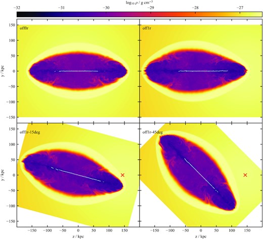
Maps of midplane density for the suite of relativistic three-dimensional simulations at |$t=32\, \textrm {Myr}$|. The slices are taken in the Y–Z plane. The upper left-hand panel shows the jets in a non-offset environment, while the remaining three panels show jets in an environment offset by 1 core radius (|$144\, \textrm {kpc}$|). The jets in the two lower panels are inclined 15° and 45° away from the environment centre, respectively; the image panels are rotated by the corresponding amount such that the environment centre is aligned with the horizontal axis. The location of the environment centre is marked in the three offset simulations with a red cross. White contours on each plot denote an internal Mach number of 5. The primary jet is propagating towards the environment centre, in the +Z direction, while the secondary jet is propagating in the −Z direction. In the offset environments, the primary jet is propagating into a rising density and pressure profile, and produces a shorter, narrower cocoon, compared to the secondary jets. Lateral asymmetry is observed across the primary lobe when the jet is inclined with respect to the environment centre. In this case the jet head preferentially expands away from the dense centre of the environment creating a lopsided structure.
In Fig. 4 we show midplane slices of velocity along the jet axis. The white contours (which denote a bulk velocity of 0.5c) highlight the deceleration of jet material after the disruption point. Clear backflow is present in all simulations, and slight asymmetries are introduced in the inclined jets due to the environment (the lower two panels of Fig. 4). The overall lobe shape is pinched in the case of the primary jet (see e.g. top right-hand panel of the same figure).
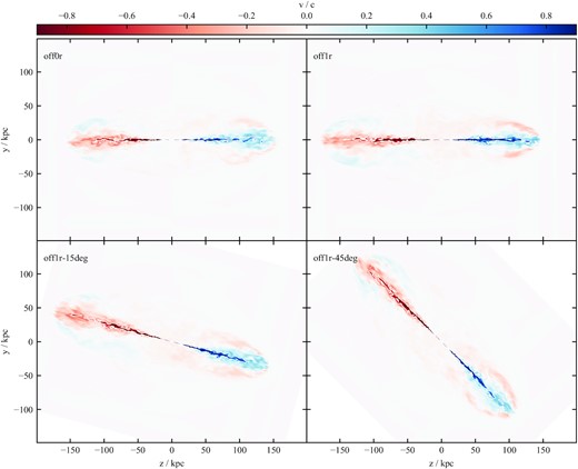
Maps of midplane velocity along the jet axis for the suite of relativistic three-dimensional simulations at |$t=32\, \textrm {Myr}$|. The slices are taken in the Y–Z plane, oriented as in Fig. 3. White contours on each plot denote a bulk velocity magnitude of 0.5c.
We measure the lobe morphology using a tracer threshold of 10−6. Gaibler et al. (2009) have shown that lobe morphologies do not strongly depend on the exact value of this parameter. Fig. 5 shows the lobe length evolution as a function of time. We also plot the lobe length evolution as modelled by RAiSE (Turner & Shabala 2015), using the same jet parameters and environment. The jets undergo a fast expansion phase for the first few Myrs, before beginning to slow; this initial ‘breakout’ phase is not captured by the RAiSE model. However, at later times, the rate of jet length evolution is consistent with the analytical model.
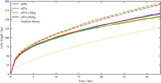
Lobe length as a function of time for all three-dimensional simulations, calculated using a jet tracer threshold. The primary lobe is shown as the solid line, while the secondary lobe is shown as the dot–dashed line. The theoretical evolution of a non-offset lobe modelled using the RAiSE analytic model (Turner & Shabala 2015) with the same jet parameters and environment is shown as the dashed line.
In all offset cases, the primary jet is shorter – as predicted by analytic theory (e.g. Kaiser & Alexander 1997) for a rising density profile – and the lobe is pinched compared to the secondary jet. This causes the observed lobe length asymmetry; initially, the primary and secondary lobes are similar, but they diverge as the source ages. Inclining the jet with respect to the cluster centre has no significant effect on lobe length.
In Fig. 6 we plot the evolution of the length and width ratios for all three-dimensional simulations. All offset simulations show significant departures from the baseline, demonstrating that the secondary lobe is becoming both longer and wider than the primary with time.
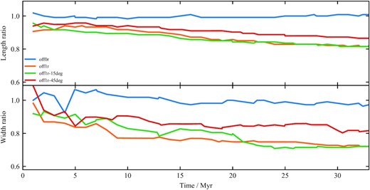
Lobe length (upper) and width (lower) ratios (primary/secondary) as a function of time for all three-dimensional simulations.
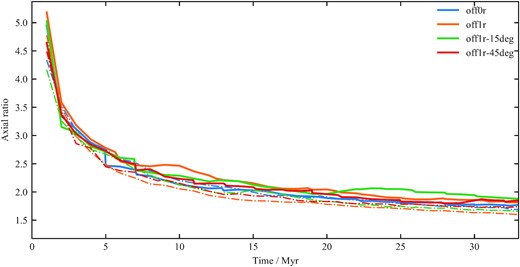
Following Hardcastle & Krause (2013) we define the lobe axial ratio as the ratio between the lobe length and the lobe width, as measured at the midpoint of the lobe; the axial ratio for all simulations is plotted in Fig. 7. The lobes produced by relativistic jets are initially elongated with high axial ratios, during the breakout phase of the jet. As the jet head propagation slows, the lobes begin to inflate because they are overpressured compared to the environment, causing the axial ratio to approach the range [1.5, 2]. This is significantly lower than in the non-relativistic simulations of Hardcastle & Krause (2013). Since a large fraction of observed axial ratios is between 1.5 and 2 (figs 6–9; Mullin, Riley & Hardcastle 2008), our relativistic jets with self-consistent hydrodynamic collimation may explain many radio sources better than non-relativistic ones, although projection effects non-trivially affect this.
Lobe axial ratio as a function of time for all three-dimensional simulations. Line styles are as in Fig. 5.
In contrast to the length and width ratio evolution, the difference in axial ratio between the primary and secondary lobes for the 1rc-offset relativistic simulations is small. At later times this difference becomes more pronounced, with the primary lobes having a consistently higher axial ratio compared to the secondary lobes. The width ratio evolution is a function of both the length ratio (as the lobe width is measured at the midpoint between the core and the hotspot), as well as the pinching occurring in the primary lobes.
Relativistic jets produce initially narrow lobes. The length evolution of the lobe is driven by balancing both the jet head pressure and momentum flux against the ambient density and pressure, while the transverse expansion is determined solely by the lobe pressure (Hardcastle & Krause 2013). All simulations have axial ratios that evolve with time, indicating that they are not expanding self-similarly, consistent with analytical models of Turner & Shabala (2015) and Hardcastle (2018).
3.2 Simulated radio emission
In addition to the purely morphological differences, the primary and secondary jets have different lossless lobe luminosities and size-luminosity tracks, as shown in Figs 8 and 9. The secondary jet has consistently higher lobe luminosities for a given time, due to the increased volume. Lobe pressure can be considered homogeneous across the entire radio source due to the high sound speed, except for the overpressured hotspots. This results in a strong correlation between luminosity and lobe volume for the lossless calculations used in this work, and so the secondary jets produce lobes with higher luminosities due to their larger volume. The luminosity evolution of all our primary lobes is very similar; the same is true for the luminosity evolution of all our secondaries. Hence, we conclude that our results are robust for variations of the angle the jet makes with the environment symmetry axis.
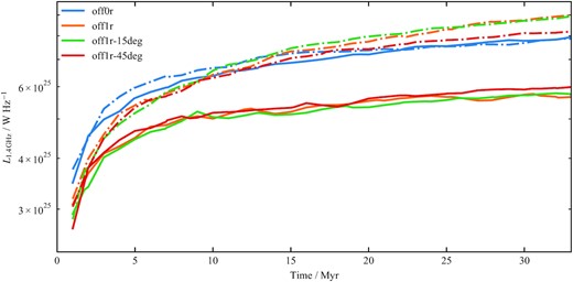
Luminosity evolution as a function of time for all three-dimensional simulations. The luminosity is calculated for an observing frequency of |$1.4\, \textrm {GHz}$| by integrating the tracer-weighted emissivity over the simulation domain. No losses are included in the emissivity calculation, so these are the upper limits of the luminosity. Line styles are as in Fig. 5.

Fig. 9 shows the impact of environment profiles on size-luminosity tracks. The primary size-luminosity tracks of the offset simulations begin to flatten out after the initial |${\sim}80 \, \textrm {kpc}$|, as the environment itself starts to flatten out. The secondary size-luminosity tracks on the other hand continue rising for the 1rc-offset simulations inclined at 0 and 15°.
We show synthetic radio images in Fig. 10. We note once more that radiative losses would make the central parts of the lobes less prominent and increase the surface brightness contrast between the hotspot and lobe. Despite the jets becoming unstable and undergoing entrainment, the general source structure is FR II-like and clear hotspots are produced. Subtle differences are consistently visible between the primary and secondary lobes. The primary jets exhibit enhanced surface brightness at the hotspots as expected from theory (Kaiser et al. 1997).

Synthetic surface brightness maps for the relativistic three-dimensional simulations at |$32\, \textrm {Myr}$|. The surface brightness is calculated for an observing frequency of |$1.4\, \textrm {GHz}$|, at a redshift of z = 0.05, observed with a 2D Gaussian beam with |$\theta _\textrm {FWHM} = 5\, \textrm {arcsec}$| and a pixel size of |$1.8\, \textrm {arcsec}^2$|. The surface brightness is shown in units of mJy per beam, and there are six evenly spaced contours in log space from |$\log _{10} \textrm {Surf.~bright.} = 1.5\, \textrm {to}\, 2.5\, \textrm {mJy~beam}^{-1}$| The primary lobe exhibits enhanced surface brightness at the hotspot, and reflects the narrower underlying cocoon.
4 COMPARISON TO OBSERVATIONS
A large number of extended radio sources show some degree of length asymmetry in their radio lobes. A large analysis of these asymmetric objects was presented by Rodman et al. (2019). The authors used a sample of mainly double-lobed radio sources identified as having asymmetric straight radio lobes through the Radio Galaxy Zoo citizen science project (Banfield et al. 2015), using data from the Faint Images of the Radio Sky at Twenty Centimeters (FIRST; Becker et al. 1995) and the Australian Telescope large Area Survey (ATLAS; Norris et al. 2006; Middelberg et al. 2008). Their final sample contained radio sources with redshift z < 0.3, selected to have approximately straight radio lobes greater than |$100\, \textrm {kpc}$| in size, with at least 20 neighbour galaxies associated through photometric redshifts to the host galaxy using the Sloan Digital Sky Survey (SDSS) DR10 (Ahn et al. 2014). Galaxies were associated with one of the radio lobes based on whether they lay within either a 45 or 90° cone aligned with the lobe major axis.
The key finding of Rodman et al. (2019) is a strong anticorrelation between the radio lobe length and number density of galaxies associated with that lobe. Use of optical galaxy clustering as a good proxy for the underlying environment is supported by Schindler, Binggeli & Böhringer (1999), who showed that the galaxy and intra-cluster gas distributions in the Virgo cluster are similar. A length-environment density anticorrelation is predicted by Kaiser & Alexander (1997; Turner & Shabala 2015), and Rodman et al. (2019) concluded that large-scale environment asymmetry is driving the radio lobe asymmetry.
In Fig. 11 we compare our simulations with data from fig. 9 from Rodman et al. (2019). Those authors plot the lobe length asymmetry of observed radio sources against the environment asymmetry as derived from optical galaxy clustering. To reproduce their plot, the lobe length asymmetry ratio is calculated at each timestep as lratio = lp/ls and plotted against the environment density ratio ρratio = ρ(lp)/ρ(ls) for each simulation. The initial environment density (given by equation 1) is used, and lp and ls refer to the primary and secondary lobe lengths, respectively. We plot the environment density ratio on the same axis as the optical galaxy clustering asymmetry ratio.
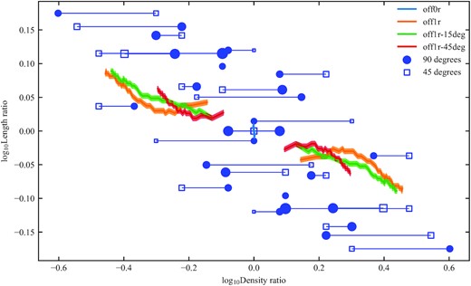
Length asymmetry ratio as a function of density asymmetry ratio using data courtesy of Rodman et al. (2019, fig. 9). The numerical simulation data for the three-dimensional simulations is shown in the same colours as Fig. 5, from t = 0 to |$t=32\, \textrm {Myr}$|. Error bands are shown for the simulation tracks, taken to be the ±1σ bounds of the 0rc-offset simulation. Observed data is represented as the closed circles and open squares, where the symbol size is proportional to the galaxy count. The observed data has been mirrored along the line y = x, to reflect the freedom in choosing the primary radio lobe. Optical asymmetry ratio calculated using a cone of 90° is shown as the closed circles, while a cone of 45° is shown as the open squares – the observed data for each radio galaxy is connected by a horizontal line.
We find that the simulations reproduce the observed anticorrelation found by Rodman et al. (2019), and fill a significant portion of observed parameter space. As the environment density asymmetry increases with source length (and hence age), these tracks show the temporal evolution of a radio source through this diagram. An estimate of the scatter in our method is given by the asymmetry tracks for the 0-offset simulations, which is confined to the very centre of the parameter space. While our simulations do not completely explain the observed asymmetries, they do reproduce the overall trend. Based on this, our results imply that a significant portion of the observed length asymmetry in radio lobes can be traced back to large-scale environment asymmetries, in agreement with Rodman et al. (2019).
5 DISCUSSION
It is important to consider the assumptions present in our simulations before summarizing our results. These simulations do not include magnetic fields; this is a valid assumption given their relatively small influence on the large-scale lobe morphology. However, magnetic fields are likely to play a role in jet stability and collimation (Matsumoto, Komissarov & Gourgouliatos 2021), something which we aim to investigate in future work. The absence of magnetic fields also necessitates an approximate radio emissivity model. The main effect of losses is to dim radio lobes in the central parts, where electrons from the oldest part of the backflow reside. Since our main interest here is the lobe morphology towards the tips of the lobes, the basic lossless model used in this work is sufficient for discussing the observable large-scale morphological differences.
Interestingly, we find that towards the end of the simulations, our jets are unstable on the 10 s of kpc scale, despite having a Lorentz factor of 5. We have convinced ourselves in two-dimensional axisymmetric control runs that this is purely a three-dimensional (and therefore realistic) effect. This is reminiscent of the three-dimensional jet disruption for low Mach number jets demonstrated in much detail by Massaglia et al. (2016). The interesting corollary here is that stable FR II jets with our chosen power (intermediate for FR IIs) require Lorentz factors higher than 5 to form a stable jet out to the 100 kpc scale. This finding is independent of the environments simulated, as jet stability is determined by the cocoon properties (density, pressure) that are similar across the different simulations.
Nevertheless, our sources have clear FR II structure from our simulated radio maps and hence the comparison to the observations is justified. As in the observations, we find that environment asymmetry translates to lobe length asymmetry. Our simulations take full account of the hydrodynamic recollimation of the relativistic jet. Hence, the system is free to adjust jet recollimation, and hence jet width dynamically with the lobe pressure, and our jets stay collimated for long enough, for that process to be simulated faithfully. Our central lobe pressures are, however, uniform enough, such that the recollimation happens similarly for both jets of a radio source. Hence, the lobe asymmetry follows the naive expectation. Significant random scatter may be added to the lobe length asymmetry from the initial interactions of the jets with the dense, stochastically clumped, interstellar medium within the galaxy (Gaibler et al. 2011).
6 SUMMARY AND CONCLUSIONS
In this work, we have presented three-dimensional simulations of powerful relativistic radio jets in an isothermal beta environment, to study the effect of asymmetric environments on large-scale lobe morphology and radio observables. These jets have varying offsets and inclination angles with respect to cluster centre; all other jet parameters are held constant. We follow their evolution from conical injection and subsequent collimation to inflation of the large-scale radio lobes. In summary, our work has shown the following:
Lobes propagating into denser environments are consistently shorter, exhibit a pinched morphology, and have enhanced surface brightness at the hotspot when compared with their counterparts.
The inflated cocoon exhibits morphology deviations with inclination angle; backflow at the primary jet head preferentially expands away from the environment centre due to the increased density. The effect is, however, rather small, and overall deviations from axisymmetry appear to be dominated by random effects of three-dimensional instabilities. The backflow is consistently narrower in the denser environment.
The jet collimation process is similar for both jets of a radio source regardless of offset and inclination angle. This is due to the homogeneous pressure distribution in the cocoon.
Our simulations reproduce the observed link between radio source asymmetry and environment asymmetry (Fig. 11). This supports the theory that jet–environment interaction plays a significant role in determining radio source morphology at large scales and opens the possibility of using radio sources as probes of the host environment in observations by next-generation survey instruments like SKA and it’s pathfinders.
ACKNOWLEDGEMENTS
We thank Aikaterini Vandorou, Geoffrey Bicknell, Dipanjan Mukherjee, and Alex Wagner for useful discussions. We also thank an anonymous referee for their useful comments. PYJ thanks the University of Tasmanian for an Australian Postgraduate Award, the ARC Centre of Excellence for All Sky Astrophysics in 3 Dimensions for a stipend, and both the University of Tasmania and the Astronomical Society of Australia for their international travel support. SS thanks the Australian Government for an Endeavour Fellowship 6719_2018. PYJ and SS thank the Centre for Astrophysics Research at the University of Hertfordshire for their hospitality
This work was supported by resources awarded under Astronomy Australia Ltd.’s ASTAC merit allocation scheme, with computational resources provided by the National Computational Infrastructure (NCI), which is supported by the Australian Government. We also gratefully thank the Tasmanian Partnership for Advanced Computing of the University of Tasmania for the computational resources provided. We acknowledge the work and support of the developers providing the following python packages: astropy (Astropy Collaboration 2018, 2013), jupyterlab (Kluyver et al. 2016), matplotlib (Hunter 2007), numpy (Harris et al. 2020), and scipy (Virtanen et al. 2020).
DATA AVAILABILITY
The data underlying this article will be shared on reasonable request to the corresponding author.
