


ABSTRACT
Active galactic nucleus (AGN) emission is dominated by stochastic, aperiodic variability which overwhelms any periodic/quasi-periodic signal (QPO) if one is present. The Auto-Correlation Function (ACF) and Phase Dispersion Minimization (PDM) techniques have been used previously to claim detections of QPOs in AGN light curves. In this paper, we perform Monte Carlo simulations to empirically test QPO detection feasibility in the presence of red noise. Given the community’s access to large data bases of monitoring light curves via large-area monitoring programmes, our goal is to provide guidance to those searching for QPOs via data trawls. We simulate evenly sampled pure red noise light curves to estimate false alarm probabilities; false positives in both tools tend to occur towards time-scales longer than (very roughly) one-third of the light-curve duration. We simulate QPOs mixed with pure red noise and determine the true-positive detection sensitivity; in both tools, it depends strongly on the relative strength of the QPO against the red noise and on the steepness of the red noise PSD slope. We find that extremely large values of peak QPO power relative to red noise (typically ∼104−5) are needed for a 99.7 per cent true-positive detection rate. Given that the true-positive detections using the ACF or PDM are generally rare to obtain, we conclude that period searches based on the ACF or PDM must be treated with extreme caution when the data quality is not good. We consider the feasibility of QPO detection in the context of highly inclined, periodically self-lensing supermassive black hole binaries.
1 INTRODUCTION
Active galactic nuclei (AGNs), driven by matter accreting on to supermassive black holes (SMBHs), are among the most powerful and steady sources of luminosity in the Universe. AGNs are luminous across the electromagnetic spectrum (EM) – bolometric luminosities can span typically 1040–1047 erg s−1 – particularly in the optical/UV regime. In many cases, emission in the radio and gamma-ray bands due to collimated jets is also observed. Since their discovery, AGNs have featured in a range of both theoretical and observational insights. Correlations between SMBH masses and both the stellar velocity dispersions and luminosities of host galaxy bulges suggest co-evolution of SMBHs and their host galaxies (Magorrian et al. 1998; Ferrarese & Merritt 2000). AGNs likely provide galaxy-scale radiative and mechanical feedback (e.g. McNamara & Nulsen 2007). Additionally, AGNs could serve as excellent testing grounds for general relativity through the investigation of dynamical accretion flows, and supermassive binary black hole systems might potentially reveal a wealth of information via multimessenger signals.
AGN continuum emission can be strongly variable on time-scales from ks to years; study of this continuum variability can elucidate characteristic time-scales that provide insight into accretion flow or jet physics. Variability mechanisms are likely linked to system parameters such as black hole mass MBH, luminosity, accretion rate relative to Eddington, etc. For example, the characteristic time-scales measured in broad-band X-ray power spectral density (PSD) functions (‘breaks’ in the continuum power-law slope; Edelson & Nandra 1999; Uttley, McHardy & Papadakis 2002; Markowitz et al. 2003) scale with both MBH and luminosity, as empirically quantified by McHardy et al. (2006). The extrapolation of this relation to stellar-mass black hole X-ray binaries (BHXRBs) – along with X-ray/radio luminosity relations (Edelson & Nandra 1999) – supports the notion of identical accretion mechanisms in both classes of objects, and leads to the interesting possibility that variability components present in one class of object may be present in the other. The X-ray PSDs of several actively-accreting BHXRBs also reveal quasi-periodic oscillations (QPOs; e.g. Wijnands, Homan & van der Klis 1999; Casella et al. 2004; Motta et al. 2015). The so-called low-frequency QPOs typically observed near frequencies f ∼ 1–30 Hz, evolve in frequency as source luminosity and inner disc size evolve and may be associated with Lense–Thirring precession in the inner disc (e.g. Ingram & Done 2012). High-frequency QPOs usually occur at 40–450 Hz; the frequencies scale as the inverse of MBH, and thus may be an imprint of MBH and spin (Remillard et al. 1999; Abramowicz & Kluźniak 2001).
The efforts to locate periodic signals (either strictly- or quasi-periodic) in both Seyfert AGN and blazars have involved studies using light curves spanning the EM spectrum. Some interpretations posit a ‘hotspot’ in the innermost accretion disc, yielding inferred constraints on the size of the inner disc or on MBH (e.g. Gupta, Srivastava & Wiita 2009). Some periodicities reported in blazars are interpreted as due to jets’ precessing in and out along the line of sight (e.g. Villata & Raiteri 1999; Li et al. 2009a; Sandrinelli et al. 2016) including modulation associated with the blazar being part of a gravitationally bound SMBH binary system (e.g. Lehto & Valtonen 1996; Valtonen et al. 2006). Additional recent claimed periods for quasars have also been interpreted as support for binary SMBH systems; luminosity variations are ascribed to modulations in the mass accretion rate caused by the binary’s orbital motion (e.g. Liu et al. 2015; Graham et al. 2015; Charisi et al. 2016).
However, statistically robust detections of strictly-periodic oscillations (SPOs) or QPOs remain a challenge. Limited data quality for AGN can pose a challenge. For example, searches for QPOs in the broad-band X-ray PSDs or periodograms1 of Seyferts is hampered by poor frequency resolution, particularly in comparison to the higher-quality X-ray timing data for BHXRBs in which QPOs are typically detected (Vaughan & Uttley 2005). Hence, so far there have been only a few robust X-ray-based claims, such as the QPO observed in RE J1034 + 396, which persists at a time-scale of ∼1 h across observations spanning years (Gierliński et al. 2008; Alston et al. 2014) a ∼2 hr QPO detected in MS 2254.9 − 3712 (Alston et al. 2015) and a ∼ 24 minute QPO in IRAS 13224 − 3809 (Alston et al. 2019); for additional detections see Ashton & Middleton (2021). However, the behaviour of the PSD – e.g. distribution and scatter of periodogram points; biases – under a variety of noise processes (white, red, etc.) and in astrophysical contexts is now well-understood (e.g. Fisher 1929; Leahy et al. 1983; Papadakis & Lawrence 1993). Particularly when data quality is high, meaning data sampling is relatively continuous (few major gaps) and close to even spacing, the periodogram or PSD is straightforward to use for detections of QPOs (e.g. Vaughan 2005). Otherwise alternate statistical methods are generally employed for the detection of periodic/QPO signals in AGN with sparsely sampled data points, such as the Auto-Correlation Function (ACF), Phase Dispersion Minimization (PDM), wavelet analysis, sinusoidal fitting, etc. Generally, QPOs claimed in AGN using these alternate methods are non-repeatable in additional observations, are based on improper usage of statistical tools, such as simply identifying the highest-amplitude points in a periodogram as outliers (e.g. Webb et al. 1988; Smith & Nair 1995; Pihajoki, Valtonen & Ciprini 2013; Ackermann et al. 2015), or improper calibration of the ‘false alarm probability.’ In particular, the presence of stochastic, aperiodic ‘red noise’ is seen at all wavebands and dominates the AGN emission and which tends to bury any possible periodic/quasi-periodic signal, if any present. In addition, pure stochastic red noise processes (no QPO present) are seen to spuriously mimic few-cycle sinusoid-like periods (Kozłowski et al. 2010; Vaughan et al. 2016), which can be misinterpreted as an intrinsic periodic signal. Hence, it is crucial to account for the amount and form of the red noise which can impact the calculation of statistical significances of detection of periods and calibration of false alarm probability while using any statistical tool. Many claims of AGN periodicities in the literature simply made no attempt to account for this red noise ‘background.’ In addition, many claims of AGN periodicities in the literature are few-cycle (e.g. Ackermann et al. 2015; Bon et al. 2016). In either of these scenarios, it is likely the claimed periodicity does not exist, and is merely an artefact of red noise. Finally, the accumulated publications of periods in AGN do not yet exhibit any obvious trend between time-scale and system parameters such as MBH or accretion rate relative to Eddington. In contrast, the continuum break time-scales in X-ray PSDs and the characteristic frequencies of low-frequency QPOs and broad Lorentzian components in BHXRBs are observed to robustly depend on MBH and/or accretion rate.
We are in the era of ‘Big Data’, with the ground-based observing programmes such as PanSTARRS, the Palomar Transient Factory, and LOw Frequency ARray (LOFAR) and near-future programmes such as the Vera C. Rubin Large Synoptic Survey Telescope (LSST), Zwicky Transient Factory (ZTF), and Square Kilometer Array (SKA) now monitor or will monitor large fractions of the sky. The resulting light-curve data bases are likely to enable period searches over 103–106 AGN simultaneously, and examples of period searches resulting from such database trawls already exist (e.g. Graham et al. 2015; Charisi et al. 2016). If false alarm probabilities for given statistical tests are not properly calibrated, then tests run on a statistically large sample can potentially yield false detection rates. Our goal is to provide guidance for AGN QPO searches and publications, so in this work, we formulate guidelines on the proper use of two commonly-used statistical methods – the ACF and Phase Dispersion Minimization (PDM) – in red noise-dominated AGN light curves. We test their efficacy in robustly distinguishing between a pure stochastic red noise process (no QPOs) and a mixture of red noise and a high-quality QPO signal.
This paper is arranged as follows. In Section 2, we review our methodology for light-curve simulations. In Sections 3 and 4, we present results for the ACF and PDM, respectively, for both pure red-noise processes and mixtures of red noise plus QPOs, for an evenly-sampled light curve. In Section 5, we explore the effects of gaps and irregular sampling patterns in the light curve while using the PDM. We review results in light of interpretation and application to physical systems in Section 6. A summary of our main results is presented in Section 6.
2 METHODOLOGY: LIGHT-CURVE SIMULATION AND INPUT PSD MODELS
Our method is to assume certain forms for the underlying PSD (continuum shape, presence/lack of QPOs), simulate light curves, run the ACF or PDM on these light curves, and accumulate statistics on whether QPOs are detected. With regards to PSD model shape, we can consider that radio-quiet AGN have highly similar accretion processes to those occurring in BHXRBs, and that variability processes in both object classes are likely to be identical. In the X-ray PSDs of BHXRBs, broad-band continuum shapes and narrow-band QPOs are frequently modelled with cut-off power-law models and/or broad or narrow Lorentzian components (e.g. Nowak 2000; Belloni, Psaltis & van der Klis 2002; Pottschmidt et al. 2003; Axelsson, Borgonovo & Larsson 2005; Grinberg et al. 2014; De Marco et al. 2015). However, in both Seyfert (disc emission dominates) and blazar (jet emission dominates) AGN, data quality for PSD measurement at all wavelengths is generally more poor compared to those for BHXRB X-ray PSDs. For Seyferts, modelling of broad-band X-ray PSDs generally suffices to use unbroken power laws or broken or slowly-bending power laws; an exception is the X-ray PSD of the Seyfert 1 Ark∼564, which is fitted with two broad Lorentzians (McHardy et al. 2007). For blazars, broad-band PSDs at multiple wavelengths have been measured to roughly follow power laws (e.g. Goyal et al. 2017; Goyal et al. 2018; Goyal 2019) or bending power laws (Chatterjee et al. 2018). In this paper, we perform all analyses assuming that the red noise PSD continuum can be modelled as a simple power law or occasionally as a broken power law, as is typical for most AGN data, and/or as is suitable for relatively limited dynamic ranges in temporal frequency. However, we advise readers to explore specific PSD continuum shapes and perform their own Monte Carlo simulations, if needed. We simulate time series similar to AGN light curves by using the algorithm developed by Timmer & Koenig (1995). In this method, non-deterministic linear time series are produced by randomizing both the phase and amplitude of the Fourier transform of the input data of an arbitrarily chosen PSD shape. The method of Timmer & Koenig (1995) produces light curves adhering to a Gaussian flux distribution; readers are referred to Emmanoulopoulos, McHardy & Papadakis (2013) for simulating light curve corresponding to arbitrary (non-Gaussian) flux distributions. For all input PSD models, we adopt the ‘RMS2/Hz’ normalization of Miyamoto et al. (1991) and van der Klis (1997).
A is the amplitude in units of Hz−1 at an arbitrary frequency of 10−6 Hz; in the X-ray PSDs of Seyferts, power is typically of order 103 − 4 Hz−1; we adopt A = 1.5 × 10⁴ Hz−1, β is the red noise power-law slope, where more positive values correspond to steeper slopes. We search for signatures in the ACF or PDM that could be mistaken for a QPO. That is, by testing a range of PSD power-law slopes β, such simulations enable us to explore the false alarm probability associated with Type I errors (false-positive detection of a QPO using ACF/PDM) for a range of pure stochastic processes.
Finally, we consider mixtures of red noise and QPO processes: We model variability whose PSD is described by the sum of a broadband power-law continuum plus a narrow Lorentzian for a range of power-law slopes and Lorentzian RMS strength.
Many signals claimed in literature e.g. for claims of QPO from SMBH binaries lack estimates of the quality factor Q and are frequently assumed to be strict periods for simplicity. For example, in self-lensing SMBH binaries, the variations in the light curves could be strictly periodic though not with consistent wave amplitude due to variations in the accretion disc continuum luminosity. However, possible effects such as additional variability modes associated with the binary orbital motional/tidal interactions or the effects of periodic streams of matter impacting the disc may contribute to quasi-periodic components in the observed emission. In the case of precessing jets of blazars, some papers (e.g. Abraham 2000; Britzen et al. 2018) describes that the precession yields strictly periodic behaviour in the resultant light curves due to periodic beaming assuming a constant input (pre-beaming) flux. But it is easy to envision how non-sinusoidal behaviour can occur: the flux that gets amplified could depend on how many individual knots are being ejected at certain phases of precession, and there can be divergence in the fluxes and ballistic behaviour of individual jet knots.
It is impossible to consider all possible light-curve sampling patterns. For our initial tests in Sections 3–5, we assume what we refer to as our ‘baseline’ sampling: evenly sampled light curves with a duration of 250 d and having one point per day, corresponding to one representative ground-based optical observing season between 115-d yearly sun gaps. In lieu of testing potential QPOs at all frequencies between 1/(250 d) and the Nyquest frequency of 1/(2 d), we choose three representative test frequencies fL: 2.0, 8.0, and 32.0 × 10⁻⁷ Hz, corresponding to time-scales of 57.9, 14.5, and 3.6 d, and spanning 4.3, 17.2, and 69.0 cycles, respectively; we refer to them low-, medium-, and high-frequency (LF, MF, and HF) QPOs (not to be confused with the LF and HF QPOs routinely identified in the X-ray PSDs of BHXRBs near typically 0.1–30 Hz and 40–450 Hz, respectively).
Finally, we neglect the effect of Poisson noise, the measurement uncertainty associated with photon counting. In the power spectrum, this noise term is a constant level of power impacting all frequencies. In the presence of red noise, its presence likely impacts only the highest frequencies, but the exact range of course depends on both red noise slope and the level of power due to Poisson noise. As this power is another source of continuum noise, the effect would be to reduce the true-positive detection likelihood for a given value of Prat, which is defined relative to the level of red noise at that frequency. Our results can thus be considered as a ‘best case’ scenario for true-positive detections in this regard. Given that each observation has a different level of Poisson noise, different red noise PSD shape, etc., testing all such scenarios is not feasible for the current paper, but we strongly encourage readers to perform their own simulations taking into account the true PSD continuum shape as it is affected by the power due to Poisson noise.
As we are testing only a few ‘representative’ sampling patterns, we leave it to users to run their own Monte Carlo simulations (MCS) of both pure red noise processes (for a range of continuum red noise model shapes, e.g. testing unbroken and broken/bending power-law models as necessary) and mixtures of red noise + QPOs, following our paper as a guide, and testing their own sampling patterns, candidate QPO frequencies, and signal-to-noise values. More specifically, users are advised to test suitable ranges of red noise shapes (both in power-law continuum slopes and normalizations), QPO test frequencies, and values of log (Prat).
3 ACF ANALYSIS FOR PERIOD SEARCHING
The z-discrete correlation function (ZDCF; Alexander 2013) is a new method to compute the CCF when the data sets are very sparsely and irregularly sampled. It uses equal population binning and Fisher’s z-transform to compute a more accurate estimate of the CCF: the resulting bias is more moderate and tends to zero as the number of points increases. We use the ZDCF for all the tests below.
The Interpolated Correlated Function (ICF) and its associated bootstrap error (ICF; White & Peterson 1994; Peterson et al. 1998) is also used for unevenly sampled data. It linearly interpolates between data points and resamples to achieve an evenly sampled light curve. The risk, as described by White & Peterson (1994), is that results can be misleading if the interpolation does not correctly approximate the intrinsic red-noise behaviour. Given that we test a wide range of red-noise power-law slopes, including slopes as steep as β = 3, we adhere to using the ZDCF.
3.1 The behaviour of the ACF for pure Lorentzian processes
In the ‘ideal’ case of strictly periodic sinusoidal oscillations without the addition of any red noise variability, the ACF is a cosine, with correlation coefficient |$\rm r_{corr} = 1$|, at time lags corresponding exactly to the period and successive harmonics of the strictly periodic signal. In Lorentzian profiles, when the quality factor Q is reasonably high (Q ≳ 3), there are still quasi-regularly spaced peaks occurring near the expected time lags for subsequent corresponding harmonics. To quantify the dispersion in peak time lag τ and |$\rm r_{corr}$|, we simulate 1000 light curves (which is sufficient to probe the 99.7 per cent confidence limit) for the pure Lorentzians spanning a range of quality factors from 1 to 120. We define the first peak as the maximum value of the ACF after the first negative-to-positive crossing and before the second positive-to-negative crossing. We determine the 99.9 per cent confidence range of τ1, τ2, |$\rm r_{corr1}$|, and |$\rm r_{corr2}$| where the subscripts 1 and 2 correspond to the fundamental peak and the second peak (second harmonic), respectively. For values of Q larger than ∼20, the dispersion in τ1 remains approximately constant as shown in Fig. 1. Hence, we use a high value of Q = 30 for all the following tests for our study. The dispersions of τ1 & τ2 for the LF, MF, & HF QPOs are given in Table 1. We see that the 99.9 per cent limits in τ1 & τ2 are within ±20 per cent, ±10 per cent, and ±4 per cent of the input value of fL for the LF, MF, and HF cases, respectively. We later use these 99.9 per cent confidence contours as the limits within to search for the first and second harmonics when we search for QPOs mixed with broad-band red noise using the ACF at each different test frequencies. We note that the 99.9 per cent limits of |$\rm r_{corr1}$| range from 0.1 to 1.0 in the LF case, while they are more constrained to values >0.45 in the MF and HF cases. The limits of |$\rm r_{corr2}$| range from 0.1 to 1.0 in the LF and MF cases, while they are constrained to values >0.4 in the HF case.
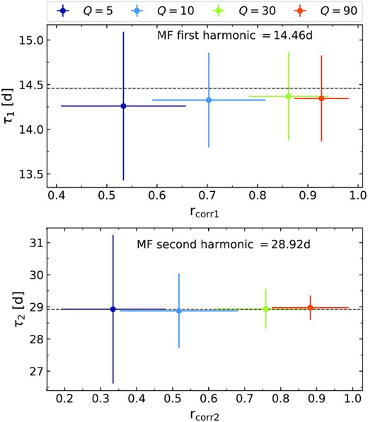
The mean and dispersion of the times of the fundamental peak (|$\rm \tau _1$|) & the second peak (|$\rm \tau _2$|) plotted against their corresponding correlation coefficient values for the MF Lorentzian signal obtained for 1000 MCS for few selected Lorentzian widths for the ACF.
The mean and dispersion of the time values of the fundamental peak (|$\rm \tau _1$|) and the second peak (|$\rm \tau _2$|) for pure Lorentzians for 1000 MCS having Q = 30 at the three test frequencies for the ACF.
| Centroid frequency | |$\rm \tau _1$| (d) | τ2 (d) | ||
|---|---|---|---|---|
| fL (10−7 Hz) | Mean (μ) | S.D (σ) | Mean (μ) | S.D (σ) |
| 2.0 (LF QPO) | 57.84 | 3.37 | 116.30 | 7.83 |
| 8.0 (MF QPO) | 14.37 | 0.48 | 28.93 | 0.61 |
| 32.0 (HF QPO) | 3.99 | 0.045 | 7.00 | 0.00 |
| Centroid frequency | |$\rm \tau _1$| (d) | τ2 (d) | ||
|---|---|---|---|---|
| fL (10−7 Hz) | Mean (μ) | S.D (σ) | Mean (μ) | S.D (σ) |
| 2.0 (LF QPO) | 57.84 | 3.37 | 116.30 | 7.83 |
| 8.0 (MF QPO) | 14.37 | 0.48 | 28.93 | 0.61 |
| 32.0 (HF QPO) | 3.99 | 0.045 | 7.00 | 0.00 |
3.2 The behaviour of the ACF for pure red noise power-law processes
3.2.1 Unbroken power-law model
We generate pure red noise light curves using an unbroken power-law PSD model for a wide range of slopes β (0.4–3.0), in steps of Δβ = 0.2 for 1000 realizations at each step.
In Fig. 2(a), we display the ACFs of a few selected light curves generated with the same power-law model, β = 2.2, but with different random number seeds. We note the appearance of spurious broad bumps and wiggles in some ACFs; some of the peaks after the zero lag can attain values of |$\rm r_{corr}$| as high as 0.8 or 0.98. For one particular realization, the green curve in Fig. 2(a), the ACF has three broad bumps wherein the second and third peaks correspond to time lags roughly 2 and 3 times the delay of the first peak. This signature is similar to that expected for a quasi-periodic signal, but it was generated by a purely stochastic process.
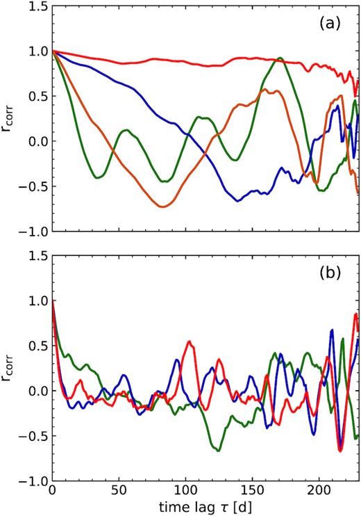
The ACFs of pure red-noise light curves generated with (a) an underlying unbroken power-law PSD that has a power-law slope of β = 2.2, and with different random number seeds. Such a pure random stochastic red noise process causes broad bumps and wiggles in the ACFs. For example, consider the green line: the first peak occurs at time lag of ∼55 days, with successive peaks near 110 and 165 d. Such a signature is similar to that expected from a quasi-periodic signal and thus can possibly misintepreted as a period, (b) for an input PSD with a broken power-law model, with slope β = 2 above a temporal frequency of 5.62 × 10⁻⁷ Hz breaking to γ = 1 below it. Again, broad bumps and wiggles are common.
As a preliminary exploration of false positives and the time-scales over which they can occur, we adopt the following criteria for false positives: only the ACF that crosses zero level at |$\rm r_{corr}=0.0$|and rises up to a non-zero value will register a positive detection at the time lag (τ1) with maximum value of correlation coefficient (|$\rm r_{corr1}$|). In this way, we have the false positives determined as a function of time lag. Again, to register a second peak, the |$\rm r_{corr}$| should drop from the maximum value corresponding to |$\rm r_{corr1}$|, cross zero and rise up again to peak at a non-zero value. That will register a second positive peak at the corresponding time lag τ2 at the second maximum correlation coefficient |$\rm r_{corr2}$| after the zero lag. For illustration, in Fig. 2(a), the green lines will register false-positive detection at time lags corresponding to three peaks, while the orange and blue line will show false positives at time lags corresponding to the first and second peak after crossing zero. The ACF in red will not register any false positives at any time lag since it never crosses zero. Because the ACF and PDM points are very highly self-correlated in the presence of red noise, determining the effective number of independent time-scales is not straightforward (in contrast to, say, an evenly-sampled periodogram). Consequently, we emphasize that our false-alarm rate tests are conducted with the goal of detecting whether or not a pure red noise process can generate *at least one* false signal *at any frequency*. This means that our derived false-alarm probabilities are conservative in the sense that the likelihood of one single signal at one given frequency being real is even lower.
In Fig. 3, we plot the distribution of false-positive peaks as a function of time-scale τ for four selected values of β. We note that the 99.9 per cent confidence distributions of |$\rm {\it r}_{corr1}$| & |$\rm {\it r}_{corr2}$| of the first and second peak become wider with increasing slope: they have |$\rm {\it r}_{corr1,2} \lt 0.45$| for β ≲ 0.8,0.6 and as the slope increases, it can range anywhere from 0 to as high as 0.9 or greater for β ≳ 1.6. This figure can be used to provide an estimate of the region of (τ1, |$\rm {\it r}_{corr1}$|) space where it is statistically likely or unlikely to encounter a false-positive peak. For a candidate peak at τ1, say, roughly 83 d =1/3 of the duration, if β = 1.0 (2.0), then only if |$\rm {\it r}_{corr1}$| is greater than roughly 0.7 (0.8) will there be a strong likelihood (>99.7 per cent) that the signal is genuine. By τ1 = 125d, 1/2 of the duration, minimum values of |$\rm {\it r}_{corr1}$| needed to confidently claim a genuine signal rise to ∼0.85 for β = 2.0.
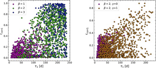
The distribution of the time scales of the first peak after the zero lag against the corresponding correlation coefficient of false positives detected in ACF for 1000 simulations of pure red noise signals of (left) unbroken PL PSD model for few selected spectral index slopes (right) broken PL PSD model for β = 2.0 breaking to few selected low-frequency slope (γ) below a temporal break frequency of 5.6 × 10⁻⁷ Hz.
Note that in Fig. 3, for slopes 2.0 and steeper (green and blue points), the majority of the false-positive peaks (τ1) occur at time-scales longer than very roughly 1/3 duration of the light curve: For β = 1.0, 2.0, and 3.0, the fractions of false peaks residing at time-scales of >1/3 duration are 261/1000 = 26.1 per cent, 790/857 = 92.2 per cent, and 316/319 = 99.1 per cent, respectively. That is, simply excluding all peaks occurring at time-scales longer than very roughly 1/3 duration is a simple and effective way to reduce the total number of false-positive detections for relatively steep red-noise slopes. When considering time-scales shorter than ∼1/3 of the duration, false-positive signals can also be minimized by excluding signal whose values of |$\rm {\it r}_{corr1}$| and |$\rm {\it r}_{corr2}$| are less than ∼0.55 and 0.45, respectively.
We also try to look for peaks without the zero crossings, i.e. the ACF which crosses any non-zero level say at |$\rm {\it r}_{corr}=0.2/0.3/0.4$| and rises up to a maximum value (i.e. |$\rm {\it r}_{corr1} \gt 0.2/0.3/0.4$|, respectively) is registered as a positive detection at the corresponding time lag (τ1). We find that even on choosing a non-zero crossing level, the red noise light curves produces significantly high percentage of false positives. For example, it shows false positives greater than 99.7 per cent (99 per cent) at β ≳ 1.2 (1.0) for the crossing level of |$\rm r_{corr}=0.2$| (0.3).
3.2.2 Broken power-law model
We generate pure red noise light curves considering broken power-law models for 1000 realizations. We study it for just few selected values of high-frequency spectral index slopes β (1.0,2.0,3.0) breaking below a temporal mid-frequency of 5.6 × 10⁻⁷ Hz to lower spectral index slopes of γ (0.0,1.0,2.0).
In Fig. 2(b), we plot the ACFs of a few selected light curves shown for a high frequency slope of β = 2.0, breaking to low frequency slope of γ = 1.0. Similar to the unbroken PL model, we see various bumps and wiggles in the ACF of broken PL model as well. The 99.9 per cent confidence distributions of |$\rm r_{corr1}$| become wider with increasing slopes of β and γ independently: for β = 1.0, 2.0 breaking to γ = 0.0, has the upper confidence limit of |$\rm r_{corr1}$| to be 0.35 and 0.45, respectively. When β = 3.0, breaking to γ = 1.0, 2.0, it has the |$\rm r_{corr}$| range from 0 to 0.98.
In Fig. 3, we plot the distribution of false positives of the first peak after zero lag for the case of β = 2.0 breaking to γ = 0.0 and γ = 1.0. We see that for the case of β = 2.0 breaking to a flatter spectrum, the majority fraction (99.2 per cent) of the candidate peaks (τ1) at time-scales < 83 d (1/3 duration) and with |$\rm r_{corr1}\lt $| 0.4, while for breaking to a more steeper spectral slope of γ = 1.0, while it still has the many of the candidate peaks (55.9 per cent) below 1/3 duration, it can still have false positives at longer time-scales with high correlation coefficient values of |$\rm r_{corr1} \gtrsim$| 0.8. Hence, we conclude that excluding peaks at time-scales longer than very roughly 1/3 duration of the light curve serves well in reducing the false-positive detections for broken-power law PSD models as well.
3.2.3 False alarm probabilities
In all discussions on errors, we consider the null hypothesis, H0, to be pure red noise variability, while the alternate hypothesis, H1, is a mixture of a QPO and red noise.
Type I error (false positive):Expanding upon the discussion from above, we calculate how often H1 is incorrectly inferred true when H0 is intrinsically true in the ACF of 1000 MCS of pure red noise light curves by using the selection criteria for false-positive detections as described in Section 3.2.1. We determine the probability of false positives of first and second peaks in the ACF across the time lag independently.
In Fig. 4, for the unbroken-PL model: When considering the full light curve duration, we notice that false positives of the first and second peak are detected with ≳ 0.3 per cent probability at all the tested values of pure red noise slope with the unbroken-PL model. For β ≲ 1.4, for example, an extremely high fraction – roughly 99.6 per cent – of all simulated light curves yield at least one false-positive signal. We also note that at relatively steeper slopes of β ≳ 2.0, the fractions of the ACF crossing zero and producing a peak becomes much lower: the ACFs of the steepest slope red noise light curves are more wide, and most of the time they never cross zero to register a false positive based on our selection criteria. Hence, the probability of finding a second peak after the zero lag also becomes smaller towards the steeper spectral index slopes.
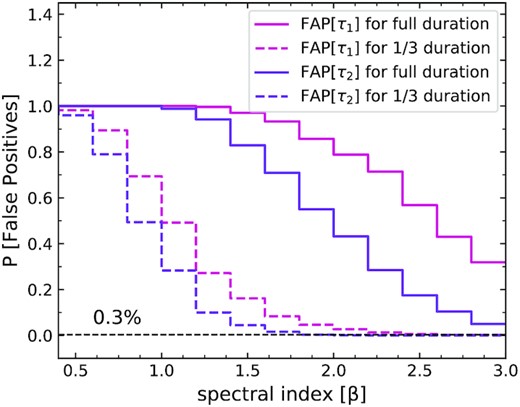
The rate of false positives detected in pure red noise light curves having unbroken power-law PSD model at different spectral index slopes for the first and second peaks in the ACF while considering the full duration and then while considering just one-third of the total duration.
As noted above in the preliminary findings, when we restrict ourselves to time-scales less than one-third of the duration, the rate of false positives of the first and second peak after the zero lag in the ACFs of unbroken-PL model is ≳ 0.3 per cent only at β ≳ 2.6, 1.8, respectively. But now, we see that less than 0.3 per cent of the simulations at all the spectral index slopes have correlation values corresponding to τ1 and τ2 greater than 0.45–0.5.
In the case of broken-PL PSD model: We tested for (i) β = 3.0 breaking to three values of γ = 0.0, 1.0, 2.0; (ii) β = 2.0 breaking to two values of γ = 0.0, 1.0; and (iii) β = 1.0 breaking to γ = 0.0, below a temporal mid-frequency of 5.6 × 10⁻⁷ Hz. When considering the full duration of the light curve in the ACF, we see that the probability of false positive of the first and second peak is >0.3 per cent for all the three cases. In fact greater than 99.7 per cent of the time, it is probable to get at least a single peak at some time lag for the cases of β = 1.0, 2.0, 3.0 breaking to γ = 0.0, 1.0. When we restrict to time-scales <1/3 duration in the ACF, we still have the false positives of the first and second peak >0.3 per cent, but the corresponding correlation values are now restricted to |$\rm r_{corr1,2} \lt 0.55$| for all the three cases. We note that particularly in the case of β = 1.0 breaking to γ = 0.0, it reaches >99.7 per cent probability of false detection for the 1000 simulations even after considering just one-third of the duration, but the maximum value of correlation coefficient that can be reached is |$\rm r_{corr1}\lt 0.35$|.
Therefore, from the above tests we conclude that by restricting to searching for peaks in the ACF at lags less than one-third of the light-curve duration and considering the first peak after the zero lag to have the correlation coefficient greater than 0.45–0.5, one can avoid the detection of false-positives and have the false-positive rates of the period of the signal to be significantly low (|$\lt 0.3{{\%}}$|) across all the spectral index slopes.
3.3 ACFs for QPOs mixed with red noise
We perform MCS for the sum of a Q = 30 Lorentzian and an unbroken power-law red noise continuum, with slopes spanning 0.4–3.0 in steps of Δβ = 0.2, and power ratios log(Prat) ranging from −1 to + 5 in steps of Δlog(Prat) = 1 for N = 1000 light curves at each step.
True-positive detections: The criteria for true-positive detections are as follows: we register true-positive detections for the first or second harmonics of the QPO independently only when they fall in their respective expected ranges of time lags as derived from the ‘ideal’ case of a Q = 30 Lorentzian (no red noise) and consider just one-third of the duration in the ACF while searching for the peaks. The corresponding correlation coefficient of the first peak also needs to have |$\rm {\it r}_{\rm corr1} \gt 0.45$|, since we need to check for the 99.7 per cent significance level to claim a true detection and to simply rule out the possibility of the peaks being due to the red noise continuum having a broken power-law model form.
We note that we do not perform the test for the LF QPO signal mixed with red noise since the distribution of |$\rm r_{\rm corr1}$| even for true Lorentzian ranges from 0.1 to 1. It is too low in order to statistically eliminate the possibility of true-positive detection from false positives (e.g. red noise with broken power law model), since we cannot restrict it along the correlation coefficient values.
The detection rate of true positives for both the first and second harmonics decreases as log(Prat) decreases and/or as the power-law slope β increases; this behaviour holds across MF, and HF QPOs, as illustrated in Fig. 5. In order to ensure a 99.7 per cent or higher reliability for detection of a QPO, one typically requires a very high power ratio. To register true positives of τ1 with 99.7 per cent significance having |$\rm r_{ corr1}\gt 0.45$|: in the MF case, log(Prat) must be 5, or 4 for values of β ≲ 2.4, or ∼1.8, respectively. In the HF case, log(Prat) must be 5, 4, or 3 for values of β ≲ 2.2, ∼1.6, or ∼1.2, respectively. To register true positives of τ2 having |$\rm r_{ corr2}\gt 0$|: for MF case, log(Prat) must be 5, or 4 for values of β ≲ 2.4, or ∼1.6, respectively (where |$\rm r_{corr2}$| is always greater than 0.2). In the HF case, log(Prat) must be 5, 4, or 3 for values of β ≲ 2.0, ∼1.6, or ∼1.0, respectively (where |$\rm r_{corr2}$| is always greater than 0.4).
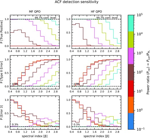
Top panel: The probability of detecting the first harmonics of the periodic signal in the expected frequency range. Middle panel: The probability of detecting the first harmonics of the quasi-periodic signal in the wrong frequency range. Bottom panel: The probability of detecting false negative of the first harmonics of the quasi-periodic signal all as a function of power ratio log(Prat) and red noise PSD power-law slope β for the MF & HF QPO mixed with broad-band red noise signals on using the ACF.
3.3.1 False negatives and detection inaccuracy errors
Type II error (false negative): H1 is inferred false incorrectly when a QPO is present.
We determine the number of times the first and second harmonics are never triggered positive (at any time-scale) in the ACF of the light curves determined independently across the time lag on using the true-positive detection criteria.
In a light curve containing a QPO mixed with red noise, to account for false negatives of the first peak, we determine the number of times not even a single peak is detected after the zero lag in the ACF (i.e. it never crosses |$\rm r_{corr} = 0$| and then rises above it) of 1000 simulations; to determine the false negatives of the second peak, we determine the number of times the ACF never crosses |$\rm r_{corr} = 0$| and rises above it after the first peak at τ1 of 1000 simulations determined independently of the time-scale of the first lag. For illustration, in Fig. 6, we plot two selected ACFs for light curves corresponding to power spectra with MF QPO signal of log(Prat) = 2 against the red noise continuum having β = 1.8. Mild features of quasi-periodicity are evident in the ACFs. The ACF shown in red in Fig. 6 has no peaks after crossing |$\rm {\it r}_{corr}=0$|. It does not satisfy our positive detection criteria and would thus lead to a false negative.
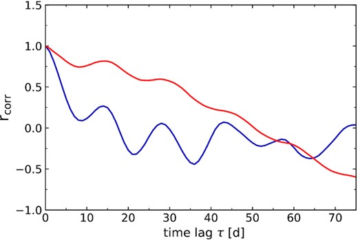
Two selected ACFs for light curves corresponding to power spectra of MF QPO signal of log(Prat) = 2 against the red noise continuum having β = 1.8. Mild features of quasi-periodicity are evident in the ACFs, but these ACF peaks do not satisfy our true-positive detection criteria and would thus lead to false negative (red) and detection inaccuracy error (blue).
Particularly for the steepest power-law slopes – β > 2 – the probability of obtaining a false negative is quite high for all but the largest values of Prat. Even for such large values of log(Prat) and large values of β, the dominating red noise causes the ACF central peak to simply not reach zero and completely overwhelms the cosine-like behaviour from the QPO.
For the MF QPO case, negligible false negative probabilities (<0.3 per cent) for the first and second harmonic are obtained only for values of log(Prat) ∼ 2, 3, 4, and 5 at β ≲ 0.6, 1.2, 1.8, and 2.4, respectively. By the time one reaches log(Prat) ∼ 1, a significant percentage (∼99.7 per cent) of simulations yield false negatives for the first (second) harmonic at β ≳ 2.8 (2.4).
For the HF case, it is a similar story: negligible false-negative probabilities for the first and second harmonic are obtained only for values of log(Prat) ∼ 2, 3, 4, and 5 at β ≲ 0.8, 1.2, 1.6, and 2.2, respectively.
False negative probabilities for the MF and HF cases are plotted in Fig. 5.
Detection inaccuracy error (Error 3): H1 is intrinsically true and also registered as true, but the QPO does not satisfy the true-positive detection criteria.
We define a detection inaccuracy error as follows: when a light curve containing a QPO mixed with red noise, produces a positive detection in the ACF, but (i) when it has the first (second) harmonic not within the ranges of time lags as derived from the ‘ideal’ case of a Q = 30 Lorentzian (no red noise) or (ii) when the correlation coefficient of the first harmonic within the expected time lag has |$\rm r_{corr1}\lt 0.45$|. For example, in Fig. 6, the ACF in blue, which corresponds to light curve having an MF QPO signal of log(Prat) = 2 against the red noise continuum having β = 1.8, has the first peak outside the frequency range expected for the MF QPO and hence will be registered as Error 3.
The probability of detecting a QPO at the wrong time-scale increases with decreasing Prat. However, with increasing power-law slope β, the probability of successfully detecting a QPO at any time-scale (within the correct range or outside of it) decreases (especially for log(Prat) ≲ 3), hence the probability of detecting a QPO at the wrong time-scale also decreases.
In general, we find that the probability of detecting the QPO (first peak) at the wrong time-scale is very low (≲ 0.3 per cent) only for values of log(Prat) ≳ 4–5 and only when avoiding the steepest values of β tested.
When log(Prat) ∼5, detection inaccuracy probabilities are <∼0.3 per cent for nearly all values of β tested: the probabilities exceed ∼0.3 per cent only for β ∼ 3.0, and ≳ 2.4 (MF and HF, respectively).
However, when log(Prat) ∼4, detection inaccuracy probabilities are <∼0.3 per cent only when β is ≲ 1.8, and 1.6 (MF and HF, respectively).
When log(Prat) ∼3, detection inaccuracy probabilities are <∼0.3 per cent only when β is ≲ 1.2 for the HF case.
The probabilities of obtaining a detection inaccuracy error for the MF and HF cases are plotted in Fig. 5.
4 PDM ANALYSIS FOR PERIOD SEARCHING
One measures the ratio of the sample variance to the overall variance of the light curve, defined as the periodogram statistic θ, given by θ = s2/σ2. It gives the measure of scatter of the sample variance about the mean of the light curve. For a true period, the scatter of the sample variance about the mean will be small, and hence we expect θ to approach zero at that frequency. For frequencies that do not correspond to a true period, the scatter of the sample variance about the mean will be large where s2 ≈ σ2 and the test statistic θ approaches 1. One can plot the test statistic θ at each trial frequency and determine the local minimum value θmin, which indicates the frequency corresponding to the least scatter about the mean light curve. It was demonstrated that the test statistic θ actually follows a beta distribution (Schwarzenberg-Czerny 1997) from which the significance of any detected pulsation can be obtained.
However, applications in astronomy have been primarily limited to situations where the underlying noise is Poisson (i.e. white noise). The performance of the PDM has not yet been empirically tested for situations where stochastic red noise backgrounds exist – it is not clear that simply identifying the local minimum value θmin automatically indicates that a strictly/quasi-periodic signal exists at that frequency.
4.1 PDM test for Lorentzian profile
We first consider the ‘ideal’ case of QPOs, as represented by simple Lorentzians centred at each of our three test frequencies and spanning a range of values of quality factor Q.
For each values of Q, we simulated 1000 light curves, again using our ‘baseline’ sampling pattern, measure their PDMs, and plot the test statistic θ determined at each trial period versus the frequency; sample PDMs for the LF, MF, and HF are plotted in Fig. 7. Each show a characteristic dip (θmin) at the expected frequency (|$\nu _{\theta _{\rm min}}$|), plus harmonics; relatively higher values of Q yield narrower dips and lower values of θmin. We plot the distributions of θmin and |$\nu _{\theta _{\rm min}}$| for LF, MF, and HF QPO in Fig. 7.
![Top panel: The PDM periodogram showing the characteristic dip at the expected frequency for one realization for different widths of Lorentzian profile at the three test frequencies. Middle panel: The histogram of the frequency $\rm \nu _{{\theta }min}$ [$\rm d^{-1}$] corresponding to the minimum statistic value $\rm \theta _{min}$. Bottom panel: The histogram of minimum statistic value $\rm \theta _{min}$ for different widths of Lorentzian profile at the three test frequencies for 1000 MCS when using the PDM.](https://oup.silverchair-cdn.com/oup/backfile/Content_public/Journal/mnras/508/3/10.1093_mnras_stab2839/1/m_stab2839fig7.jpeg?Expires=1749930595&Signature=rzJMuUe-TBQJvz48yWgoFVnz1NeEVlhtFXfRxSl2K4SxnTwNqz55p2sgtL~fYIX-85bSPLOp9DjHYtQgozBOt4M~U0MNCl0-Av2o4iPBiRrr76H3LncBFSlCHgZJZBrtHjasC8pNz8oguh9msORoEdRG6fD2-9d9LbHNaTWAuQ4d52ZJePcGhcZX6I2pJiGjNY0xb8V21WglboM6EumI7n8ITVKmfNj5gHjlKQWHhHrLNFdlkDkSEUgKWbXLvFiXaV1OGH4igqWzvKibmHiZBwpLSmV64ODqwn4kQwbaQaeO-~SSSoCla~haExPDliniP17EbRIoJcQ1-RJf5W-Elg__&Key-Pair-Id=APKAIE5G5CRDK6RD3PGA)
Top panel: The PDM periodogram showing the characteristic dip at the expected frequency for one realization for different widths of Lorentzian profile at the three test frequencies. Middle panel: The histogram of the frequency |$\rm \nu _{{\theta }min}$| [|$\rm d^{-1}$|] corresponding to the minimum statistic value |$\rm \theta _{min}$|. Bottom panel: The histogram of minimum statistic value |$\rm \theta _{min}$| for different widths of Lorentzian profile at the three test frequencies for 1000 MCS when using the PDM.
The standard deviation of |$\nu _{\theta _{\rm min}}$| decreases as Q increases. Extremely coherent signals – values of Q of order 10–20 – are typically needed to attain values of θmin below ∼0.3 for the LF and MF cases; for the HF case, values of Q closer to 90 are required.
Henceforth, we consider Lorentzians with values of Q = 30. To delineate the region of frequency–θ space where the ‘ideal’ signal occurs, we determine the 99.9 per cent confidence regions from the MCS denoting the distributions of θmin (upper limits) and |$\nu _{\theta _{\rm min}}$|; those upper limits/ranges are listed in Table 2.
The 99.9 per cent contour limits of θmin and trial frequency |$\nu _{\theta _{\rm min}}$| for the Lorentzians at the three test frequencies.
| upper limit on |$\rm \theta _{min}$| (|$99.9\,{\rm per\,cent}$|) | Range of |$\nu _{\rm \theta _{min}}$| (|$\rm d^{-1}$|) (|$99.9\,{\rm per\,cent}$|) | |
|---|---|---|
| LF QPO | 0.684 | 0.0096–0.0216 |
| MF QPO | 0.805 | 0.0608–0.0754 |
| HF QPO | 0.883 | 0.262–0.293 |
| upper limit on |$\rm \theta _{min}$| (|$99.9\,{\rm per\,cent}$|) | Range of |$\nu _{\rm \theta _{min}}$| (|$\rm d^{-1}$|) (|$99.9\,{\rm per\,cent}$|) | |
|---|---|---|
| LF QPO | 0.684 | 0.0096–0.0216 |
| MF QPO | 0.805 | 0.0608–0.0754 |
| HF QPO | 0.883 | 0.262–0.293 |
We will later use these confidence ranges as the limits within which to search for signatures of QPOs when we consider mixtures of a QPO and red noise while using the PDM.
4.2 The behaviour of the PDM for pure red noise processes
4.2.1 Unbroken and broken power-law models
We again generate pure red noise light curves using an unbroken power-law PSD model for a wide range of slopes β (0.4–3.0), in steps of Δβ = 0.2, simulating 1000 light curves at each step, and measuring their PDMs.
We determine the periodogram statistic θ across all the possible test frequency for each light curve. The resulting 99.9 per cent confidence lower limits on θ at each trial frequency are plotted in Fig. 8 for the different spectral index slopes. For all power-law slopes, θ is typically >0.9 across a wide range of frequencies, and even >0.8 down to ∼0.02 d−1 (i.e. the scatter variance is generally large above this frequency). At the lowest frequency bins however (at frequencies corresponding to time-scales longer than ∼1/3 of the duration), θ plunges to 0.6 or lower, with relatively steeper PSD slopes reaching values of θ well below 0.2 and these local minimum due to pure red noise can be misintepreted as quasi-periodic signals. In fact, we note that the fraction of pure red noise-only trials that can attain a value of θmin < 0.6 is greater than 99.7 per cent at β ≥ 2.6 and it is less than 0.3 per cent at β ≤ 0.8. However, after excluding the frequencies towards the lowest bin (at about 1/3 of the duration), we see that the fraction of pure red noise-only trials that can obtain a θmin < 0.6 is less than 0.3 per cent almost across all the tested beta values.
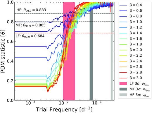
The overplot of the 99.9 per cent lower limit of the PDM statistic value |$\rm \theta$| at each test frequency that can be caused due to pure red noise light curves having evenly sampled data for broad-band spectral index slopes against the 99.9 per cent contour limits of |$\nu _{\theta _{\rm min}}$| and the upper limit on the θmin determined for pure Lorentzian signals at the three test frequencies for 1000 MCS within which we expect the characteristic dip to occur for QPOs mixed with red noise.
We repeat the test for pure red noise light curves considering broken power-law models for 1000 realizations. We study it for just few selected values of high-frequency spectral index slopes β (1.0, 2.0, 3.0) breaking below a temporal mid-frequency of 5.6 × 10⁻⁷ Hz to lower spectral index slopes of γ (0.0, 1.0, 2.0). Similar to the unbroken power-law models, we see that towards the lower frequency bins θ gets minimized to <0.6. The fractions of red noise light curves that could reach θmin < 0.6 is less than 1 per cent when any value of β breaks to flatter slope of γ = 0.0, but the fractions get higher as β increases (>40 per cent) on breaking to γ = 1.0 or 2.0. After excluding the lowest bin frequencies (corresponding to ∼1/3 duration), we see that the fraction of pure red noise-only trials that can obtain a value of θmin < 0.6 is less than 1 per cent for all the combinations of broken power-law PSD model.
It is very clear that low values of θ in a given PDM do not automatically mean that a QPO is present,since red noise can also generate such low values of θ. In particular, however, one must take into account the frequency regime where the minimum occurs before attempting to decide if a given minimum corresponds to a genuine QPO. For example, in Fig. 8, we see that at time-scales ∼1/7–1/12th of the total duration, the 99.9 per cent lower limit of θmin due to pure red noise ranges between 0.8 and 0.88, which are below the 99.9 per cent upper limit of θmin that can be reached by the HF pure Lorentzian signals but they do not occur within their expected frequency range. In fact, we note that the 99.9 per cent lower limit of θmin caused due to pure red noise never intersects with the 99.9 per cent search contour limits obtained for the MF and HF pure Lorentzian signals because it is always greater than 0.89 around those frequency bins. On the other hand, the pure red noise light curves (e.g. β < 1.2) can get θ ≲ 0.6 within the 99.9 per cent contour limits of |$\nu _{\theta _{\rm min}}$| expected for a pure LF Lorentzian signals. Hence, we will not to be able to statistically distinguish a LF QPO signal mixed with red noise causing the minimized θ value.
4.2.2 False alarm probabilities
Type I error (false positive): We calculate how often H1 is incorrectly inferred true when H0 is intrinsically true from the 1000 MCS of pure red noise light curves generated for a range of spectral indices. We determine the rate at which a pure red noise light curve can minimize the test statistic to low values at ANY frequency, with at least one occurrence per realization and can be falsely registered as a QPO signal.
We register the number of times θmin for a given PDM drops below the 99.9 per cent upper confidence limit of θmin obtained from the ‘ideal’ (Lorentzian-only) case of HF QPO having the highest value of 0.88, for each realization of the red noise light curves, to determine the probability of the false positives. In the case of unbroken power-law model as shown in Fig. 9, we see that the rate of false positives is >0.3 per cent at all the tested β values. When we neglect the lower frequency bins corresponding to time-scale >1/3 duration, even though the rate of false positive is still >0.3 per cent at all slopes, we see that there is a decrease in the rate of false positives especially towards the higher spectral index slopes. We also see a slight increase in the rate of false positives at spectral index slopes 0.6 ≲ β ≲ 1.4 because around these spectral index slope values, the red noise has 0.65 < θmin < 0.8 at frequency bins corresponding to time-scales ∼1/3–1/9 duration. In the case of broken power-law model, the rate of false positives is >0.3 per cent for all the tested combinations of β = 1.0, 2.0, 3.0 breaking to γ = 0.0, 1.0, 2.0 towards the lower frequency after the break at the mid-temporal frequency before and after excluding the lower frequency bins.
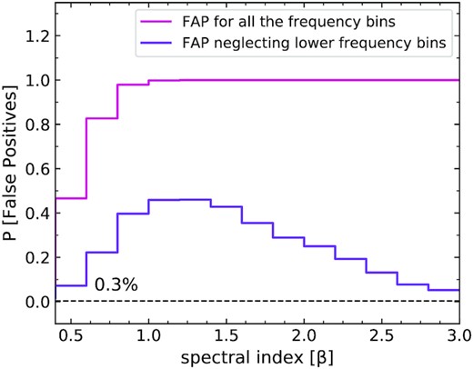
The rate of false positives detected in pure red noise light curves having unbroken power law PSD model at different spectral index slopes while using the PDM tested for all the trial frequency bins and then neglecting the lower frequency bins corresponding to time-scales >1/3 duration.
It is important to note that after neglecting the lower bins, less than 0.3 per cent fractions of red noise simulations having unbroken and broken power-law model can attain a value of θmin ≲ 0.65 and 0.5 on using the PDM for all the tested values of slopes, respectively.
4.3 The behaviour of PDM for QPOs mixed with red noise
Once again, we perform MCS for the sum of a Q = 30 Lorentzian and an unbroken power-law red noise continuum, with slopes spanning 0.4–3.0 in steps of Δβ = 0.2, and power ratios log(Prat) ranging from −1 to +5 in steps of Δlog(Prat) = 1.
True-positive detections: We register true-positive detections when |$\rm \theta _{\rm min}$| falls into the 99.9 per cent confidence range in θ-frequency space as determined from the ‘ideal’ (Lorentzian-only) scenarios above. For example, in Fig. 10, we plot the PDM periodogram for few realizations of light curve having an MF QPO signal mixed with red noise of β = 2.6. The black points are the lowest minimum (θmin) for a given PDM periodogram and the green shaded region is the 99.9 per cent contour limits of the ‘ideal signal’ in the θ-frequency space expected for the MF QPO signal. Hence, only those points which falls into this region will be registered as true positives.
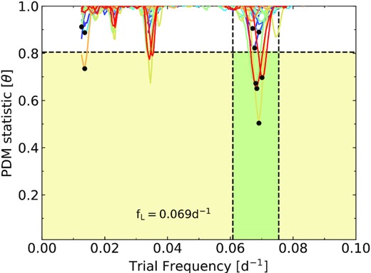
The PDM statistic θ measured at each trial frequency bin for light curves having an MF QPO signal mixed with red noise having unbroken power-law model of slope β = 2.6 of log(Prat) = 2, on using the PDM while neglecting the lower frequency bins corresponding to ∼1/3 duration. The black points represent the lowest minimum (θmin) for a given PDM periodogram and the green shaded region is the 99.9 per cent contour limits of the ‘ideal signal’ in the θ-frequency space expected for the MF QPO signal.
We find that in order to ensure that the probability of correctly registering true positives with ∼99.7 per cent, one always requires an extremely high value of log(Prat): typically >5 or more. We see that in the case of MF QPO, the signal is not detectable with the 99.7 per cent significance. As shown in Fig. 11 for the MF QPO, values of log(Prat) ∼ 4, 5 only approach reliable detections of about 99 per cent when β ≲ 1.8, 2.4, respectively, of which >85–90 per cent fraction of the simulations has θmin < 0.65. Finally, for the HF QPO, values of log(Prat) ∼ 4, 5 has 99.7 per cent significance detections when β ≲ 1.6, 2.0, respectively, and log(Prat) ∼3 only approach reliable detections of about 99 per cent when β ≲ 1.0. In the case of HF QPO signals mixed with red noise >30–40 per cent fraction of the simulations with reliable detections has θmin < 0.65.
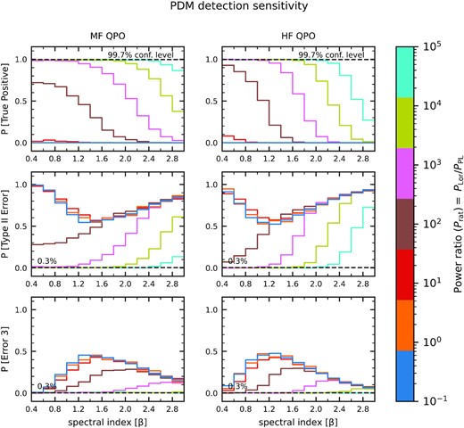
Top panel: The probability of detecting the first harmonics of the periodic signal in the expected frequency range. Middle panel: The probability of detecting the first harmonics of the quasi-periodic signal in the wrong frequency range. Bottom panel: The probability of detecting false negative of the first harmonics of the quasi-periodic signal all as a function of power ratio Prat and red noise PSD power-law slope β for the MF and HF QPO using PDM.
The above analysis was performed considering values of θmin occurring at any frequency while excluding all frequencies less than a frequency of ∼0.012 d−1, which corresponds to one-third of the duration. We also repeated the analysis including the lowest frequency bins, but this action did not yield significant changes to the results of significant detection of the period. In fact, excluding the lowest bins helps only in reducing the detection inaccuracy error of registering θmin at the wrong frequency (i.e. towards the lower bins) which will be explained in Section 4.3.1.
4.3.1 False negatives and detection inaccuracy errors
Type II error (false negative): H1 is inferred false incorrectly when a QPO is intrinsically present
When the value of θmin does not fall below the upper limit threshold determined from the ‘ideal’ case (regardless of frequency), we register that trial as a false negative. For example, in Fig. 10, some of the black points that represent the lowest minimum (θmin) for a given PDM periodogram obtained for light curves having MF QPO mixed with red noise lie above the upper limit on θ (0.805) below which MF QPO signals are expected. Hence, they will be registered as false negative.
As shown in Fig. 11, for the MF QPO, the type II error rate is below ∼0.3 per cent for values of log(Prat) ∼ 5, or 4 when β ≲ 2.4, or 2.0, respectively, and for the HF QPO, the false negative rate is ≲ 0.3 per cent for values of log(Prat) ∼ 5, 4, 3 when β ≲ 2.0, 1.6, 1.0, respectively. We see that with decreasing log(Prat) and/or increasing steepness β, the rate of the false negatives increases. We note that at log(Prat) ≲ 2, the rate of false negatives increases towards the lower spectral slopes of β ≲ 1.4. This is because at the lower power values of QPO against the red noise, the probability of finding a minimum θ at the expected contours for the MF & HF signals decreases which in turn increases the rate of false negatives around these region.
Detection inaccuracy error (Error 3): H1 is intrinsically true and also registered as true, but the QPO is detected at the wrong frequency.
We register detection inaccuracy errors when θmin falls below the upper limits derived in the ‘ideal’ case, but also falls outside the expected frequency bounds. For example, in Fig. 10, the black points which are the lowest minimum (θmin) for a given PDM periodogram obtained for light curves having MF QPO mixed with red noise, lies below the upper limit on θ (0.805), but does not lie within the expected frequency range for MF QPO. Therefore, when we have θmin of the PDM periodogram occurring in the yellow shaded region, then it is registered as Error 3.
When one blindly searches for θmin across all frequencies, including in particular the lowest frequency bins, the probability of encountering a detection inaccuracy error is generally very high, and it increases towards higher values of β and/or lower values of log(Prat). Now, when we neglect these lower frequency bins, the rate of finding the θmin at the wrong frequency bins decreases both along the log(Prat) and the spectral index slope values. In Fig. 11, we see that even though the rate of detection inaccuracy error is >0.3 per cent, it is still significantly low (≲1 per cent) at log(Prat) ∼ 4–5, for β ≲ 2.6 for both the MF and HF QPO.
5 REALISTIC UNEVEN SAMPLING PATTERNS
The AGN light curves that we get from observations are usually unevenly sampled, and typically contain data gaps and/or irregular sampling. It is thus important to explore the effects of sampling patterns when using the ACF and PDM for searching for periodic signals. It is impossible to explore all types of potential sampling patterns, so here we choose representative sampling patterns that could plausibly be observed by ground-based optical large-area surveys such as LSST, PanSTARRS, ATLAS, etc. – continuous monitoring quasi-regularly, but interrupted by yearly sun-gaps of a few months – or ground-based radio surveys such as OVRO – continuous monitoring usually year-round, with no major gaps, but with somewhat irregular sampling. We check how irregular sampling and the presence of regular gaps such as yearly sun gaps impact the signatures of pure red noise processes and impact detectability of a QPO when it is mixed with red noise.
We conduct Monte Carlo simulations of 10 yr long light curves similar to a generic optical survey such as LSST or ATLAS, first with evenly sampled data with and without different yearly sun gaps, and then we test different irregular sampling patterns, again with and without the yearly sun gaps. We perform this analysis only for a subset of the parameters explored above, as this section is intended as an exploration of the effects of only basic facets of irregular data sampling. Particularly for more complex data sampling patterns, readers are strongly encouraged to conduct their own simulations following our work as an example.
5.1 PDM test for Lorentzian profile
We repeat the analysis as in Section 4, where we first consider the ideal case of QPOs only, represented by simple Lorentzians of quality factor Q = 30. We start with evenly sampled data, assuming 10-yr long light curves having a sampling rate of one point every day. In lieu of testing potential QPOs across all frequencies between 1/(3650 d) and the Nyquest frequency of 1/(2 d). We choose three representative test frequencies fL: 1.3, 5.77, and 22.04 × 10⁻⁸ Hz, corresponding to time-scales of 2.3, 0.55, and 0.144 yr, and spanning 4.3, 18.2, and 69.5 cycles, respectively; we refer to them low-, medium-, and high-frequency (LF, MF, and HF) QPOs.
We first simulate light curves to determine the region of frequency–θ space where the ‘ideal’ signal occurs. We determine the 99.9 per cent confidence limits on θmin (upper limits): 0.705, 0.769, and 0.864 for the LF, MF, and HF QPOs, respectively; |$\nu _{\theta _{\rm min}}$| (lower, upper bounds) are (0.0005, 0.0014), (0.0045, 0.0055), and (0.0181, 0.0204) for the LF, MF, and HF QPO, respectively. These values delineate the ranges within which to search for signatures of QPOs when we consider mixtures of a QPO and red noise.
Similarly, we determine the 99.9 per cent confidence limits on θmin and |$\nu _{\theta _{\rm min}}$| first for the unevenly sampled data having different average sampling rates of 2–10 d in steps on 2, 20, and 30 d; and then for evenly sampled data and irregularly sampled data (avg. sampling rate of 8 d) having sun gaps of different values (36.5 d, 0.5–4.5 yr in steps of 0.5 yr). We see that the range of frequency–θ limits are about the same – with only ∼4–6 per cent deviation – as the values for evenly sampled data.
5.2 The behaviour of the PDM for pure red noise processes
We perform MCS for each of the different sampling patterns of red noise process of unbroken power-law PSD model and see the effect in the PDM compared to the evenly sampled data.
Even sampling pattern: We again generate pure red noise light curves using an unbroken power-law PSD model for a wide range of slopes β (0.2–3.0), in steps of Δβ = 0.2, simulating 1000 light curves at each step for the evenly sampled data for 10 yr duration having one point per day, and measure their PDMs.
The resulting 99.9 per cent confidence lower limits on θ at each trial frequency are plotted in Fig. 12. In the figure, we see that the PDM looks similar for the evenly sampled data as in Section 4.2.1 where θ reaches very low values. We notice that at time-scales about 1/3rd–1/4th of the duration of the light curve, there is a turnover in the values of the statistic minimum value where it starts to get below 0.85–0.8 and with increasing time-scale. The statistic minimum can reach lower than 0.5 at much longer time-scales (≲ one-half the duration) and can get even as low as 0.2 when PSD slopes are ≳ 1.8.
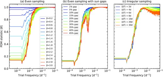
The distribution of the 99.9 per cent lower limit of the PDM statistic value |$\rm \theta$| at each test frequency of pure red noise 10 yr long LSST type light curve for (a) evenly sampled data at different spectral index slopes, (b) evenly sampled data with yearly sun gaps of 45 per cent data gap for |$\rm \beta = 2.0$|, (c) irregularly sampled data having different average sampling rate for red noise slope |$\rm \beta = 2.0$|.
Even sampling with yearly sun gaps: Now we test the effects of yearly sun gaps in the evenly sampled light curves in the PDM. So we produce 1000 light curves of unbroken power-law PSD model having slope of β = 2.0 for each different range of gaps from 1 per cent of the duration corresponding to 0.1 yr and slowly increasing the amount of gap in steps of 5 per cent of the duration corresponding to a range of 0.5–4.5 yr of gap in the 10 yr long data for demonstration on the effects of sun gaps. In Fig. 12, we plot the 99.9 per cent confidence lower limits on θ at each trial frequency for each different gaps. We see that as the amount of gap in the data increases, it produces an extra feature, where there is a sudden dip in the |$\rm \theta _{min}$| which can get lower than 0.7 at frequency ∼ 1/(365 d), when the gaps are greater than 35 per cent of your complete data apart from the deep minimum observed towards the lowest frequencies (≲1/3 of the duration), which are not significantly affected by the sun gaps.
Again, to see the effect of different slopes of red noise with data gap in the PDM, we produce red noise light curves using an unbroken power-law PSD model for a wide range of slopes β (0.4–3.0), in steps of Δβ = 0.2, having 45 per cent gap in the data, simulating 100 light curves at each step and find the 99.9 per cent confidence lower limits on θ at each trial frequency for the different spectral slopes. The dip at a frequency of 1/(365 d) becomes stronger for relatively steeper PSD slopes, including falling below ∼0.8 for values of β steeper than ∼1.2.
We thus recommend to avoid the frequency space corresponding to lower than roughly 1/3–1/4 of the duration of the light curve, as well as other obvious time-scales range corresponding to the period of the gaps, as these time-scales can see spurious deep minimum features in the PDM.
Irregular sampling: Here, we test the effects of irregular sampling without any large data gaps. We again simulate 10-year long light curves with daily sampling, but we resample by randomly selecting points every |$\rm {\Delta } T$| days, where we explore average values of |$\rm \langle {\Delta }T \rangle =$| 2, 4, 6, 8, 10, 20, and 30 d. We assume β = 2.0, and we again produce 100 light curves and determine the 99.9 per cent confidence lower limits on θ at each trial frequency; the results are plotted in Fig. 12. Here, it is the relatively higher temporal frequencies that are affected: particularly for |$\rm \langle {\Delta }T \rangle \sim$| 20–30 d, |$\rm \theta _{min}$| consistently departs from just under unity to roughly 0.95–0.87 for frequencies corresponding to time-scales shorter than roughly 1/20 of the duration. However, no narrow-band artefacts are induced.
Irregular sampling with yearly sun gaps: We test the effects in the PDM for the combination of irregular sampling and yearly data gaps. For an input unbroken power-law PSD model β = 2.0, we determine the 99.9 per cent confidence lower limits on θ at each trial frequency for each of the different average sampling rate having 10 per cent wide data gaps and then 45 per cent wide data gaps (the latter is not uncommon for many ground-based optical programmes for targets near the equator). As shown in Fig. 13, for the 10 per cent wide gap case with irregular sampling there is not much difference in the PDM compared to when there are no data gaps. For 45 per cent wide data gaps, we again see the spurious dip near time-scales of 1/(365 d) as before.
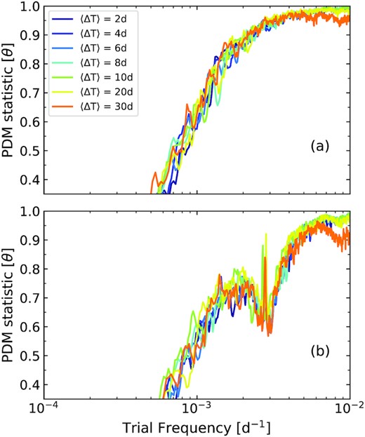
The distribution of the 99.9 per cent lower limit of the PDM statistic value |$\rm \theta$| at each test frequency for a randomly sampled pure red noise light curve having spectral index slope β ∼ 2.0 with (a) 10 per cent yearly gap and (b) 45 per cent yearly gap for different average sampling rates.
5.3 The behaviour of PDMs for QPOs mixed with red noise
We perform MCS for the sum of a Q = 30 Lorentzian and an unbroken power-law red noise continuum, with slopes spanning 0.4–3.0 in steps of Δβ = 0.2, and power ratios log(Prat) ranging from −1 to +5 in steps of Δlog(Prat) = 1, now for the 10 yr long light curves for each of the different sampling patterns. For brevity, we test only the MF QPO, though results were qualitatively similar for the HF QPOs.
We test for evenly sampled data for the 10 yr long light curve having one point per day to check for the detection probability along the different spectral index slopes and along the different power ratios. We find that the MFQPO has a detection sensitivity range of significant detection of 99.7 per cent only at log(Prat) ≳ 5.
We repeat the test for different uneven sampling patters (a) even sampling with yearly sun gaps of 40 per cent, (b) random sampling pattern having an average sampling rate of 8 d and (c) random sampling having an average sampling rate of 8 d with yearly sun gaps of 40 per cent for the 10 yr long light curve to check for the detection probability along the different spectral index slopes and along the different power ratios. We see that the detection sensitivity for the different sampling patterns to be the same as when it was evenly sampled and thus we conclude that for the PDM, sampling artefacts do not play a significant role in true-positive QPO detection sensitivity.
6 DISCUSSION
Through extensive Monte Carlo simulations of quasi-periodic processes and mixtures of quasi-periodic and red noise processes, we empirically explored the regions of parameter space where a (true-positive) detection of a QPO with the ACF or PDM is statistically robust.
We also empirically explored the signatures produced by pure red noise processes when using the ACF and the PDM, and quantified the regions of parameter space where false positives are likely to be encountered.
The light-curve sampling patterns we explored are admittedly limited in number but relevant to long-term (multiyear) observing programmes with sustained monitoring, and with sampling patterns relatively poorer than that required for a DFT. With these sampling patterns, we generally find the following:
In studying the effect of pure-red noise processes in the ACF, assuming an unbroken power-law PSD model and evenly sampled data, we see that pure red noise can produce false positives determined across the time lag at a rate more than 0.3 per cent for all tested values of the spectral index slope, which is significantly high to be neglected. In fact, correlation coefficients of the first peak can easily reach above 0.5–0.7 at β ≳ 1.4, and can reach even higher values (∼0.9) at steeper slopes of β ≳ 2.2. The second peak after the zero lag determined across the time lags independently can also have a correlation value ∼0.7 at β ≳ 1.0 and are easily misintepreted as an QPO signal at these corresponding time lags.
One can robustly avoid peaks with correlation coefficients above 0.45–0.5 caused by pure red noise by restricting oneself to lags less than roughly 1/3 of the light curve duration and thus have the false-positive rate across the time lags to be |$\lt 0.3{\rm {per\,cent}}$| while searching for a QPO signal mixed with red noise. A broken power-law input PSD (e.g. breaking from slopes from β = 2.0 to γ = 1.0 or to 0.0) yield qualitatively similar results.
In the analysis of pure red noise processes in the PDM, assuming an unbroken power-law PSD model and evenly sampled data, we see that towards the lower frequency bins – corresponding to time-scales longer than roughly one-third of the duration – |$\rm \theta$| consistently dips below 0.8–0.85. In fact, about 99.7 per cent of the pure red noise simulations with PSD slope of β ≳ 2.4 can yield values of |$\rm \theta _{min}$| below 0.6. Therefore, it is to be noted that low values of θ in a given PDM do not automatically mean that a QPO is present e.g. at low frequencies.
After excluding the lowest bin frequencies (corresponding to longer than 1/3 of the duration), we see that the fraction of pure red noise-only trials that can attain a value of θmin < 0.6 is less than 1 per cent for all the tested combinations of broken and unbroken power-law PSD models. Hence, merely neglecting the lower frequency bins in the PDM is a straightforward way to minimize false-positive detections.
We considered mixtures of red noise processes and a Q = 30 QPO, and explored detection sensitivity ranges in both the ACF and PDM for a range of red noise slopes and QPO strengths relative to the red noise (quantified by log(Prat)), neglecting time-scales >1/3 duration, we find the following:
Detection of the period with statistical significance (|$\gtrsim 99.7{\rm {per\,cent}}$|) depends strongly on both the strength of the QPO against the red noise and the steepness of the red noise PSD slope. In general, the probability of detection of the signal at the correct period gets lower with increasing steepness of the red noise slope and decreasing power of the QPO against the red noise.
Particularly for relatively steep PSD slopes, extremely large values of log(Prat) are required for robust detections of a QPO in both the ACF and PDM.
For illustration, in Fig. 14, we have the light curve corresponding to power spectra of MF QPO signal of log(Prat) = 2 against the red noise continuum having β = 1.8. Even if mild features of quasi-periodicity are evident in the light curves, these power values of QPO would likely not register a true-positive detection in either the ACF (52.3 per cent likelihood of not registering a true-positive detection) or PDM (86 per cent likelihood of not registering a true-positive detection) at any time-scale.
With the ACF, we generally find that QPOs are detected robustly only when log(Prat) ≳ 5 for β ≳ 2.4/2.2 for a MF/HF QPO, respectively. Detections at values of |$\rm log(P_{rat}) \sim 3$| are attainable only at lower spectral index slopes, β ≲ 1.2.
For the PDM, we require |$\rm log({\it P}_{rat}) \sim$| 4, 5 for β ≲ 1.8, 2.4 even for a 99 per cent detection for MF QPO. Detections at values of |$\rm log(P_{rat}) \sim 4, 5$| are possible for β ≲ 1.6, 2.0 for the HF QPO.
We explore the effects of regular data gaps and irregular sampling in the PDM. Irregular data sampling causes |$\rm \theta _{min}$| to become low (∼0.95) across broad swaths of frequencies, but true-positive detection rates for mixtures of QPOs with red noise are not significantly impacted. When a regular data gap such as a yearly sun gap are included, it produces a relatively narrow-band feature that is confined to e.g. 1/(365d).
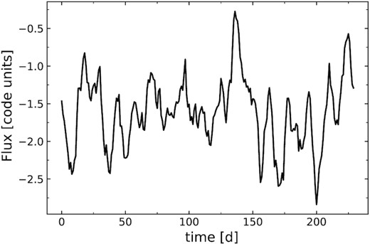
A sample light curve corresponding to power spectra of MF QPO signal of log(Prat) = 2 against the red noise continuum having β = 1.8, where mild features of quasi-periodicity are visually evident in the light curve. However, such a light curve would very likely (likelihood) yield no detection with an ACF or PDM.
When there is a claim of a QPO signal from AGN in the literature, then one should be able to not just articulate its frequency and rms, but also the form of the underlying red noise continuum and the uncertainties related to these parameters. In the case of ACF/PDM, it is not easy to determine the underlying PSD shape. We conclude that since the ACF/PDM tend to produce false alarm rates greater than |$0.3{{\%}}$| and given the general quality of AGN data gathered so far, it is advisable that the community should be cautious and refrain from publishing claims of QPO using the ACF/PDM (until they have a reliable and significant detection considering proper null hypothesis), since the detection rate is generally low and not significant until one reaches very high values of power of QPO against the red noise continuum.
In Section 6.1, we briefly discuss some of the main problems affecting many of the claims of periodicities in the literature in AGN. In short, they include (1) sampling too few cycles of a ‘signal’, as red noise can produce spurious sinusoid-like trends on the longest time-scales, and/or (2) mistreatment of the null hypothesis: white noise, or red noise with insufficiently steep power-law slope, is assumed; the likelihood of false positives tends to increase towards steeper PSD slopes.
Another issue regarding claims in the literature, though, is that there is rarely any mention of the inferred rms or rms/mean (hereafter referred to simply as RMS for simplicity) of the claimed periodic signal. While the value of the period of course encodes physical info about the variability mechanism, so does the RMS of the QPO; if parameter constraints from other analyses are known, a consistency check can further help test if the claimed QPO is real. We discuss this topic further, with a couple brief applications, in Section 6.2.
6.1 Some of the claims in the literature and basic pitfalls regarding ACF and PDM usage
One major caveat in searching for QPOs against a red-noise background, as pointed out by e.g. Vaughan et al. (2016), is that pure red noise processes, particularly those with relatively steep PSD slopes (β > ∼2), can produce quasi-sinusoid-like, ‘W-shaped’ segments of light curves for three or four ‘cycles.’
For observations of a finite length of a red noise process, the dominant trends on time-scales longer than (very roughly) one-third of the full duration may be quasi-sinusoidal. These trends can potentially ‘trick’ any period-searching method – ACF, PDM, fitting sinusoidal functions to light curves – into falsely identifying a period, without a proper calibration against a null hypothesis in place (e.g. Press 1978).
In this paper, we empirically quantify how pure red noise processes can produce false signatures in both the ACF and the PDM reminiscent of those produced by a pure Lorentzian signal – strong correlation peaks in the ACF, and dips in θmin in the PDM – particularly on time-scales longer than roughly one third of the light curve duration.
The problem of observing too-few cycles can potentially be resolved by extending observations. For example, Graham et al. (2015) claimed a period of ∼1900 d in an optical light curve of the quasar PG 1302–102 by sinusoidal fitting of a ∼10-yr light curve; Vaughan et al. (2016) demonstrated the light curve’s consistency with pure red noise. Moreover, an additional five years’ monitoring reported by Liu, Gezari & Miller (2018) failed to confirm this period.
A second major caveat is that developing and testing a proper null hypothesis (pure red noise, no QPO) is critical for testing the statistical significance of a candidate period (especially in the absence of having the luxury of being able to extend monitoring). Testing against a null hypothesis consisting of Poisson (instrumental) noise only is clearly insufficient; some papers such as Li et al. (2009b) do not attempt any such significance test. We empirically see that with both the ACF and PDM, the likelihood of encountering a false positive from a pure red noise process is extremely sensitive to the value of the underlying power-law PSD slope, and false positives can be significant in number particularly for β > ∼2. We recognize that it can be difficult to measure a periodogram and obtain an unbiased fit when data sampling is poor, but having at least a roughly accurate idea of β is thus critical for being able to form a proper null hypothesis.
Below we briefly discuss these warnings in the context of using the ACF and PDM, and point out some examples in the literature of misinterpretation. Our intention is not to single out individual authors; our intention is to simply focus on discussing common mistakes, citing a few select examples in the literature only. A caveat is that data sampling in these cited publications are always not exactly the same as in our simulations in terms of dynamic range of frequencies explored, frequency resolution, number and size of data gaps, and the irregularity of data sampling. In addition, estimates of power-law slope β are usually difficult to know reliably, sometimes because data were too sparse for a reliable periodogram fit. However, we believe that differences in sampling should not significantly impact our qualitative conclusions about these works. Moreover, these works each have data sampling such that the ratios of maximum to minimum temporal frequencies probed is usually of order a few hundred, roughly similar to what we explored in this paper.
6.1.1 General issues with ACF, with a few select examples
One basic problem with attempting to use the ACF for period-searching, as demonstrated in Section 3.2, is that pure red noise processes can produce spurious bumps and wiggles at all time-scales (particularly relatively longer time-scales and when β > ∼1.5) which might be mistaken for a QPO signature.
ACFs in citations claiming a QPO frequently do not show the clear cosine-like behaviour expected when a QPO dominates; both Li et al. (2009b) and Fan et al. (2002), for instance, simply identify multiple local peaks in their ACFs as candidate signals, but these are likely artefacts of red noise, e.g. with β ∼ 1 − 2.
Raiteri et al. (2001, 2021) and Liu et al. (2011) and each claim QPO signatures in peaks occurring at time-scales >1/3 – ∼1/2 of the light-curve durations, with values of rcorr peaking at ∼0.5–0.7. However, we demonstrated that for both unbroken power-law PSDs with β > 1.4 and broken power-law PSDs, rcorr can frequently peak above 0.7 (and rcorr can even frequently peak above 0.9 when β > ∼2.2 very easily, especially at time-scales > 1/3 of the duration. For Liu et al. (2011), the fundamental issue is that their light-curve samples 2.5 cycles of a sinusoid-like trend (‘W-shape’) and is consistent with red noise likely corresponding to a very steep PSD slope, probably β ∼ 2 or 3.
6.1.2 General issues with PDM, with a few select examples
One basic issue with attempting to use the PDM for period searching was demonstrated in Section 4.2: pure red-noise processes yield spuriously low values of θmin at relatively low frequencies / long time-scales e.g. >∼ 1/3 of the light-curve duration. For example, even in the limit of perfect data sampling, red noise processes across all range of β tested can cause θmin to drop to below values of typically e.g. ∼0.80–0.85 below a frequency corresponding to ∼30 per cent of the duration for the sampling patterns and red noise slopes simulated in this paper.
In the literature, claims of periods hinge on observed localized minima in the PDM, but these minima tend to occur towards long time-scales, >∼1/3–1/4 of the duration: Fan et al. (2002), Liu et al. (2011), and Peñil et al. (2020).
Note that Liu et al. (2011) and Fan et al. (2002) have used the Jurkevich (1971) method, which is numerically related to the PDM: both calculate the sample variance within each test phase bin and consider the sum of those variances. However, the PDM is normalized by the overall variance in the light curve. Meanwhile, Fan et al. (2002) and Li et al. (2009b) used a renormalized Jurkevich parameter |$V^2_{\rm m}$| following Kidger, Takalo & Sillanpaa (1992), defining a fraction |$f \equiv (1 - V^2_{\rm m})/V^2_{\rm m}$|, but it does not take into account the number of degrees of freedom; the expectation value in the absence of any periodicity consequently can differ significantly from 1. In this paper, we do not simulate the Jurkevich method specifically, and a direct comparison of our values of θmin to values of |$V_{\rm m}^2$| as a function of time-scale is not immediately straightforward. None the less, given the characteristics of pure red noise processes, claims of periods occurring at long time-scales using either method should be relatively suspect.
6.2 Application to detection of periods for selected physical situations
When there exists a periodic signal mixed with red noise in the emission from a source, and if the red noise power spectral characteristics can be estimated, then, for a given sampling pattern and a given test frequency, the threshold values of power ratio required for a successful detection of a periodic signal with statistical significance using PDM or ACF can be translated into threshold values of rms for the periodic component.
Such threshold values can be used to define the regions of parameter space for a given physical system where a periodic signal can be detected with the PDM or ACF. Alternately, for a given input set of parameters for a periodically induced signal, one can estimate the rms and then power ratio of the signal against the red noise continuum, and compare to threshold values of log(Prat) that can be detected with the PDM or ACF. Moreover, given the high minimum values of log(Prat)needed for detection as demonstrated by this paper, whenone claims detection of a periodic signal using the ACF or PDM, they are implicitly claiming a minimum value for log(Prat) and thus rms – and these values have implications for the physical parameters of a given system.
Here, we briefly discuss the application to periodically self-lensing SMBH binaries in highly inclined systems on using the results from ACF and PDM.
6.2.1 Highly inclined self-lensing SMBH binaries
We consider highly inclined super massive black hole (SMBH) binary systems following the framework of D’Orazio & Di Stefano (2018, hereafter DD18). Emission from the accretion disc around the primary black hole is periodically gravitationally lensed and magnified by the secondary. For simplicity, we assume that our simulations results, derived assuming QPOs with a very high quality factor, are applicable to such strictly-periodic systems. SMBH binary systems could additionally have quasi-periodic emission, potentially. Hydrodynamic simulations of accretion on to SMBH binaries from circumbinary discs can yield quasi-periodic fluctuations in accretion rate through the circumbinary disc (e.g. Farris et al. 2014; Farris et al. 2015). If such variations in accretion rate directly yield variations in luminosity when that material accretes on to the black holes, then quasi-periodic components contributing to observed emission might be expected.
However, tests incorporating mixtures of QPOs and red noise (including that generated in the two accretion mini-discs) would be difficult, because predicting the degree and PSD shape of the contaminating red noise is quite challenging: there could be additional modes of variability not present in stable/ more persistently accreting discs; one would need to know the radii over which those variability mechanisms are triggered, taking into account e.g. tidal truncation of the outer discs (e.g. Paczynski 1977; Nguyen & Bogdanović 2016). Consequently consideration of red noise (from mini-discs) with QPO mixtures in this context is beyond the scope of our paper.
We consider just the optical and UV emission from the inner accretion disc. We use Breedt (2009, their fig. 5.3) as an empirical guide for optical PSD slopes and normalization. Breedt (2009) publish V-band unbroken power-law PSDs for seven Seyferts; we take the average value of slope (β = 2.3) and normalization (20 Hz−1 at |$\rm 10^{-6}$| Hz).
We note that any possible evolution with black hole mass (MBH) or accretion rate relative to Eddington LBol/LEdd (as is known for broadband X-ray PSDs of nearby Seyferts, e.g. McHardy et al. 2006) is not accounted for here. Any given SMBH binary system may very likely host black holes with differing values of black hole masses and if both the black holes in the binary system are accreting, then LBol/LEdd might also differ and yield different individual PSD shapes and/or normalizations, and the sum of their variability characteristics will be reflected on the single optical PSD shape that we measure. Hence, for extreme simplicity, we neglect such effects and assume that the single PSD shape represents the level of red noise emission from both systems.
We adopt from DD18 magnification factors for binary systems having mass ratios q = 0.05 and q = 0.5, and having the accretion discs that are nearly edge-on, with inclination J = 0.2 rad with respect to the line of sight. We consider each of the NUV and V bands separately; the former represents a more ‘optimistic’ case in terms of the magnification. We adopt the waveforms in Fig. 3 of DD18 to estimate the rms/mean for each of four binary orbital inclinations to the line of sight in units of the number of Einstein radii, NE, which quantifies the angular separation of source and lens at closest approach, corresponding to NE = 0.05, 0.1, 0.5, and 1.0. A magnification factor is not the same as a change in flux, since the input flux from the accretion disc, which is stochastic, will vary with time. For simplicity, though, we ignore this effect. Values of rms/mean are listed in Table 3.
The values of rms/mean estimated from the light curves of highly inclined SMBH binary systems, based on the flare emission profiles in DD18. Listed here are values for two selected values of mass ratio, four selected values of NE, the fraction of an Einstein radius separating the lens and the source at closest approach, and two wavebands, NUV and V. Also listed, in parentheses, are estimates of log(Prat) assuming a mixture of a Q = 30 QPO at the MF QPO frequency, 8.0 × 10⁻⁷ Hz, and a continuum PSD with β = 2.3 and a normalization of 20 Hz−1 at 10−6 Hz.
| Mass ratio q = 0.05 | Mass ratio q = 0.5 | |||
|---|---|---|---|---|
| NE | NUV | V | NUV | V |
| 0.05 | 0.752 (5.67) | 0.471 (5.27) | 0.784 (5.70) | 0.504 (5.33) |
| 0.1 | 0.471 (5.27) | 0.281 (4.82) | 0.504 (5.33) | 0.307 (4.89) |
| 0.5 | 0.095 (3.87) | 0.074 (3.66) | 0.105 (3.96) | 0.082 (3.75) |
| 1.0 | 0.030 (2.88) | 0.030 (2.88) | 0.033 (2.96) | 0.033 (2.96) |
We simulate 250-d long continuous monitoring light curves that are evenly sampled, assuming a Q = 30 QPO at the MF frequency used in Sections 3–5, 8 × 10⁻⁷ Hz, and considering each of the values of rms/mean for each inclination/waveband/mass ratio combination, mixed with a β = 2.3 continuum PSD as per the parameters listed above. For simplicity, we assume the same continuum PSD parameters for both the V and NUV bands. The resulting values of log(Prat) are listed in Table 3; they span from roughly 2.9 for the NE = 1.0 cases up to 5.7 for the NE = 0.05 cases.
Recall, however, from Section 4, Fig. 11 that when using the PDM, for β = 2.3, values of log(Prat) of 5 were required for robust true-positive detections at ∼99 per cent confidence for the MF QPO. For the ACF, values of log(Prat) of 5 were required for robust true-positive detections at ≳ 99.7 per cent confidence; the NE = 0.05 and 0.1 cases would thus likely be detected. (Note: we choose to be approximate in our conclusions here given the large uncertainties and assumptions regarding the form of the continuum PSD as discussed above.)
Note that we are commenting on the possibility of detections in individual systems only; determining the frequency of occurrence of such systems whose orbital parameters satisfy these requirements is beyond the scope of this paper.
7 CONCLUSIONS
In this paper, we have presented results from an empirical investigation of the behaviour of two statistical tools – the ACF and the PDM – when used for detecting a QPO in light curves that contain broadband stochastic red noise variability.
These tools have been used to claim the presence of periodic signals in AGN light curves; however, pure red-noise processes can easily mimic features that could falsely be interpreted as a QPO. Guidance in both preventing false-positive QPO claims and in supporting true-positive detections is needed, particularly given that the astronomical community now has, or will have access to databases containing large numbers of monitoring light curves courtesy of current and near-future large-area ground-based monitoring programmes such as LSST.
This paper is intended to provide guidance both to those examining individual light curves for QPOs and to those performing data trawls in large databases. Our overarching goal is to help reduce the appearance of false claims of periodocities (features consistent with the null hypothesis of simple red noise) in the literature.
We perform Monte Carlo simulations covering a range of red noise power-law PSD slopes and QPO strengths for a few select light curve sampling patterns. We empirically investigate both true-positive detections of QPOs when mixtures of broadband red noise and a narrow-band QPO are present and false-positive detections when no QPO is present, only red noise (the null hypothesis model).
We determine that pure red noise light curves tested for a broad range of power-law slopes were able to produce false-positive signals in the ACF more than 0.3 per cent of the time at all slopes tested, considering the full time-scale range. False-positive peaks routinely reach correlation coefficients of 0.5 and higher. When we restrict ourselves to lags less than one-third of the full duration, the rate of false positives still remains ≥0.3 per cent at power-law slopes β ≳ 2.6, though maximum correlation coefficients remain below 0.55. We conclude that if one observes a peak with correlation coefficient >0.5 and while restricting oneself to lags less than roughly 1/3 of the duration, and given even data sampling, then the signal is probably real.
In the case of the PDM, pure red-noise processes cause a dips in the value of the PDM test statistic θ (e.g. θ < ∼0.6), particularly at frequencies corresponding to time-scales greater than roughly one third of the duration. The rate of false positives is greater than 0.3 per cent across all the tested slopes, and at much steeper slopes β ≳ 1.4, false positives occur almost 99.9 per cent of the time. However, when we simply neglect the lowest frequencies (time-scales greater than roughly one third of the duration), the rate of false positives is still greater than 0.3 per cent for all the slopes, but having the PDM statistic θ below 0.65 is <0.3 per cent. Hence, neglecting the lower frequency bins in the PDM is a straightforward way to minimize false-positive detections.
These results are an empirical demonstration that, when using the ACF or PDM, and when variability due to a pure red noise process with an unbroken power-law PSD shape, the ad hoc action of simply disregarding time-scales greater than ∼1/3 of the full duration is an effective way to reduce false positives (we strongly caution, however, that this one-third benchmark is meant to be highly approximate only, and can depend on e.g. steepness of power-law slope, data sampling, etc.). They also suggest that features occurring at the longest time-scales/lowest frequencies in previously published ACFs/PDMs may have been consistent with pure red noise instead of being due to QPOs, as claimed.
When there are QPOs mixed with pure red noise in evenly sampled data, the true-positive detection sensitivity in both the ACF and PDM naturally depends strongly on not just the relative strengths of the QPO and the red noise [log(Prat)] but also sensitively on the steepness of the red noise PSD slope. We find that extremely large values of log(Prat) typically 4–5 without the pre-filtering technique introduced in Sections 3.3 and 4.3 – are typically required for a 99.7 per cent true-positive detection rate, at PSD slope – β typically <∼2.
The reader is reminded that we did not add Poisson noise to our simulated light curves; this would likely make a true-positive detection even more difficult, so our results are effectively lower limits to values of log(Prat).
We re-iterate that any claim of a QPO detection using the ACF or PDM implies detection of a signal with such a high power ratio. Depending on the model applied for interpretation, it is possible that the high values of log(Prat) and rms imply extreme regions of model parameter space. For example, in the specific case of periodically self-lensing black holes in gravitationally-closed binary systems on a highly inclined orbit that we considered in Section 6.2, values of log(Prat) ≳ 5 (assuming no light-curve filtering) in optical/UV emission from the inner disc require the source and lens to be separated by only NE ∼ 0.05 at closest approach (DD18).
We also examined a small range of different sampling patterns, including yearly sun gaps as is common to ground-based optical observing programs, and irregular but sustained sampling, and their effect on true- and false-positive detection rates in the PDM; True-positive detection rates for a given values of log(Prat) and β are not significantly impacted.
If readers who are searching for QPOs have light curves with sampling patterns identical to those we simulated, then we encourage those readers to use our simulations and plots as guides to determining whether features in their own ACFs/PDMs are indicative of any QPO or are consistent with a single pure red noise process.
If readers have light curves with different sampling patterns, and/or want to test a null hypothesis model more complex than a simple unbroken power-law, then we recommend that they perform their own simulations, including testing the range of behaviour that can be exhibited under the appropriate null hypothesis model, depending on the slope of the underlying red noise process (and its uncertainty). If the slope is not known specifically, then readers should test a wide range of slopes in order to be conservative. As a final reminder, we did not consider the effects of Poisson noise in our simulations here, and readers should take that into account in their own simulations.
It is worth considering whether or not a periodogram is more efficient at cleanly separating broad-band continuum noise from a narrow-band QPO compared to the ACF or PDM for a given sampling pattern.
For evenly sampling data, the method of Vaughan (2005) is applicable for QPO detection in a periodogram, and the behaviour of the periodogram (probability distribution of powers, biases, the extent to which adjacent temporal frequencies are independent, etc.) has been well understood (see references in e.g. Vaughan 2005).
However, for a given rms strength, the value of log(Prat) needed to register a detection of a QPO will depend on factors such as temporal frequency spacing and the quality factor Q. For unevenly sampled data, other factors come into play for all methods, such as the impact of aliasing at high temporal frequencies, which depends on spectral slope and data sampling. Such detailed discussions are beyond the scope and intent of the present paper, but we encourage readers who have a specific sampling pattern in mind to perform simulations for all methods to help gauge detection rates of both true and false positives. We would like to warn users of the ACF and PDM that it is not possible to use these tools to reliably separate a narrow-band signal and the red noise continuum and quantify the form of that continuum, since the presence of red noise causes the ACF and PDM values to become highly self-correlated.
We would thus encourage the community to consider testing of additional methods, including Bayesian fits (e.g. CARMA; Zhu & Thrane 2020), and development of automatic light curve classifiers (e.g. Sánchez-Sáez et al. 2021) that could potentially quantify deviations from pure-red noise behaviour. However, comparison testing of how the various methods – be they classical such as ACF, PDM, periodogram, or modern – perform in maximizing true-positive detections and minimizing false detections is beyond the scope of the current paper.
Finally, we strongly encourage readers to report the implied value of the RMS (or equivalently, rms/mean) of the QPO, in addition to time-scale, in any future QPO claims they publish, regardless of the statistical method used. The rmsn codes additional information about the physical parameters of the periodic process and/or variability mechanism (e.g. observer viewing angles; jet angle parameters; energy dependence of a variability mechanism), yet such information is regularly neglected in published QPO claims. Hopefully, physical parameters implied by the QPO strength will be consistent with physical information obtained from other avenues methods (imaging, spectroscopy), if available.
ACKNOWLEDGEMENTS
SK, AM, and ASC acknowledge support from Narodowe Centrum Nauki (NCN) grant no. 2016/23/B/ST9/03123. SK and AM also acknowledge partial support from NCN grant no. 2018/31/G/ST9/03224. SK and AM thank T. Bogdanovic for useful discussions on applications to physical systems.
DATA AVAILABILITY
The data underlying this article will be shared on reasonable request to the corresponding author.
Footnotes
The periodogram is an estimator of the PSD.
REFERENCES
APPENDIX
The parameter space for significant detection of the period of the MF and HF QPO signals mixed with red noise of unbroken PL model on using the ACF tested for evenly sampled light curves in Section 3.
| PARAMETER SPACE for significant detection on using the ACF | |||
|---|---|---|---|
| Centroid frequency | True positives | Type ii error | Error 3 |
| fL (10−7 Hz) | (|$99.7\,\rm{per\,cent}$|) | (|$\lesssim 0.3 \,\rm{per\,cent}$|) | (|$\lesssim 0.3 \,\rm{per\,cent}$|) |
| 8.0 (MF QPO) | log(Prat) ∼ 5/4 at β ≲ 2.4/1.8 | log(Prat) ∼ 5/4 at β ≲ 2.4/1.8 | log(Prat) ∼ 5/4 at β ≲ 3.0/1.8 |
| 32.0 (HF QPO) | log(Prat) ∼ 5/4/3 at β ≲ 2.2/1.6/1.2 | log(Prat) ∼ 5/4/3 at β ≲ 2.2/1.6/1.2 | log(Prat) ∼ 5/4/3 at β ≲ 2.4/1.6/1.2 |
The parameter space for significant detection of the period of the MF and HF QPO signals mixed with red noise of unbroken PL model on using the PDM tested for evenly sampled light curves in Section 4.
| Parameter space for significant detection on using the PDM | |||
|---|---|---|---|
| Centroid frequency | True positives | Type II error | Error 3 |
| fL (10−7 Hz) | |||
| 8.0 (MF QPO) | log(Prat) ∼ 5/4 at β ≲ 2.4/1.8 (|$99\,\rm{per\,cent}$|) | log(Prat) ∼ 5/4 at β ≲ 2.4/2.0 (|$\lesssim 0.3 \,\rm{per\,cent}$|) | log(Prat) ∼ 5/4 at β ≲ 2.6 (|$\lesssim 1\,\rm{per\,cent}$|) |
| 32.0 (HF QPO) | log(Prat) ∼ 5/4/3 at β ≲ 2.0/1.6/1.0 (|$99.7\,\rm{per\,cent}$|) | log(Prat) ∼ 5/4/3 at β ≲ 2.0/1.6/1.0 (|$\lesssim 0.3\,\rm{per\,cent}$|) | log(Prat) ∼ 5/4 at β ≲ 2.6(|$\lesssim 1\,\rm{per\,cent}$|) |
