


ABSTRACT
Most ultraluminous X-ray sources (ULXs) are thought to be powered by super-Eddington accretion on to stellar-mass compact objects. Accretors in this extreme regime are naturally expected to ionize copious amounts of plasma in their vicinity and launch powerful radiation-driven outflows from their discs. High spectral resolution X-ray observations [with reflection grating spectrometer (RGS) gratings onboard XMM–Newton] of a few ULXs with the best data sets indeed found complex line spectra and confirmed such extreme (0.1–0.3c) winds. However, a search for plasma signatures in a large ULX sample with a rigorous technique has never been performed, thereby preventing us from understanding their statistical properties such as the rate of occurrence, to constrain the outflow geometry, and its duty cycle. We developed a fast method for automated line detection in X-ray spectra and applied it to the full RGS ULX archive, rigorously quantifying the statistical significance of any candidate lines. Collecting the 135 most significant features detected in 89 observations of 19 objects, we created the first catalogue of spectral lines detected in soft X-ray ULX spectra. We found that the detected emission lines are concentrated around known rest-frame elemental transitions and thus originate from low-velocity material. The absorption lines instead avoid these transitions, suggesting they were imprinted by blueshifted outflows. Such winds therefore appear common among the ULX population. Additionally, we found that spectrally hard ULXs show fewer line detections than soft ULXs, indicating some difference in their accretion geometry and orientation, possibly causing overionization of plasma by the harder spectral energy distributions of harder ULXs.
1 INTRODUCTION
1.1 Ultraluminous X-ray sources
Ultraluminous X-ray sources (ULXs; Kaaret, Feng & Roberts 2017) are non-nuclear point sources in nearby galaxies with an isotropic luminosity exceeding 1039 erg s−1, the Eddington luminosity of a standard 10 M⊙ stellar-mass black hole. The nature of ULXs was an open question for decades, with two scenarios being that they are either powered by sub-Eddington accretion on to the elusive intermediate mass black holes (Miller et al. 2003; Farrell et al. 2009) or by super-Eddington accretion on to stellar-mass compact objects (King et al. 2001; Poutanen et al. 2007; Gladstone, Roberts & Done 2009; King 2009).
Now, we know that a majority of these objects is powered by super-Eddington accretion. A crucial piece of evidence for this hypothesis was the discovery that at least some ULXs are pulsating and thus are unambiguously powered by neutron stars (Bachetti et al. 2014; Fürst et al. 2016; Israel et al. 2017a,b; Carpano et al. 2018; Sathyaprakash et al. 2019; Rodríguez Castillo et al. 2020). Furthermore, ULX X-ray spectra are substantially different from the typical spectra of sub-Eddington accreting systems because of a high-energy roll-over at energies less than 10 keV (Bachetti et al. 2013; Walton et al. 2014).
Moreover, powerful outflows with velocities of up to 20–30 per cent of the speed of light were discovered in several ULXs through detection of highly blueshifted atomic features seen in absorption (Pinto, Middleton & Fabian 2016; Walton et al. 2016; Pinto et al. 2017; Kosec et al. 2018a), including evidence for an outflow in a neutron star powered ULX (Kosec et al. 2018b). Radiation-driven disc winds are naturally expected to arise in super-Eddington accretion (Shakura & Sunyaev 1973; Poutanen et al. 2007) and are therefore an important piece of evidence towards our understanding of the nature of ULXs.
1.2 Automated spectral search methods
Any ionized plasma, which may or may not be part of the outflowing wind, will imprint spectral lines on the continuum X-ray spectrum of the ULX. If the plasma lies along our line of sight towards the X-ray source, it will absorb X-ray photons, producing absorption lines. Otherwise, it will produce emission lines. If the plasma is in motion with respect to us, the observed line wavelengths will be Doppler-shifted from their rest-frame wavelengths.
Considering that any detected spectral feature could then be Doppler-shifted, it is not always straightforward to identify it, in particular if the expected shifts can be large (which is the case here). Similarly, it is not easy to assign a statistical significance to any line detection – in other words, it is not straightforward to calculate the probability that the detected line originates from noise rather than from optically thin plasma near the ULX. Given the low X-ray fluxes of ULXs (due to their Megaparsec distances), these features can often appear to be just on the limit of significance. Thus, it is important to estimate their significance accurately.
This is a complex problem that must be approached systematically. An automated routine is necessary in order to search the source X-ray spectrum and locate any possible spectral lines. Then, the algorithm needs to calculate the statistical probability that each of the tentatively detected features is real and does not originate from noise.
Such methods have recently been developed and successfully applied to detect outflows in a few ULXs (Pinto et al. 2016, 2017) and in active galactic nuclei (AGN; Cappi et al. 2009; Tombesi et al. 2010; Kosec et al. 2020b). These methods directly fit the X-ray spectra in spectral fitting packages such as spex (Kaastra, Mewe & Nieuwenhuijzen 1996) and xspec (Arnaud 1996) in an automated fashion. The simpler versions of the routines scan the spectra with Gaussian lines (Kosec et al. 2018a) and thus are used to detect absorption and emission lines. The more complex versions (Kosec et al. 2018b; Pinto et al. 2020b) search the spectra with large grids of physical models and are therefore able to identify and fit many absorption/emission lines simultaneously (accounting for their Doppler shifts) and infer the plasma physical properties.
These methods are very powerful in locating the best-fitting spectral features (lines or absorbers/emitters), however, they become computationally expensive when one needs to assess the statistical significance of the detections. A search of a spectrum for spectral features will often locate many spurious features that might appear significant. This is simply because a large parameter space has been searched, increasing the chances that it contains a strong feature originating from pure noise (Vaughan & Uttley 2008). This is called the look-elsewhere effect. To account for such effect, one must repeat the search many times on simulated data sets with statistics comparable with the real data, but containing just Poisson noise superimposed on the featureless broad-band continuum of the X-ray source. The false positive rate of any detected feature is then the fraction of simulated data sets containing fake features equal to or stronger than the one detected in real data.
As a result, to test for reasonable significances (∼3σ) one has to perform a few 1000s Monte Carlo searches on simulated data sets, which can be very computationally expensive (>1000 computer hours). This kind of analysis is therefore only possible on a very small number of sources.
Here, we make an important point regarding the line significances. All of the above only applies to completely random and unexpected features, i.e. lines that occur at wavelengths that do not belong to known and expected rest-frame elemental transitions. If a line is detected at a known transition and such transition is a plausible origin for the feature (no Doppler shift expected or the Doppler shift is known), the possible parameter space for its identification collapses and the line significance can be approximately (but not exactly, as shown by Protassov et al. 2002) determined directly from spectral fitting without the need for Monte Carlo simulations. In this case, the required line strength for detection significance is much lower. For a line with fixed wavelength (to the elemental transition rest-frame) and fixed width, this is a problem with a single extra free parameter (the line normalization), and thus a fit improvement of ΔC-stat = 9 or Δχ2 = 9 results in 3σ detection significance. Given the extreme conditions near the ULX, the number of plausible elemental transitions in the soft X-ray band is in fact quite small. Due to the high temperatures involved, the ULX spectra will likely only show a handful of K and L shell transitions of a few abundant elements such as Mg, Ne, Fe, O, and N.
1.3 This work
In this work, we study all ULXs with high enough quality X-ray data, and search their high-resolution spectra for any emission or absorption lines, while quantifying the true statistical significance of any features detected. All the detected features are included in a single catalogue, thus creating the first catalogue of spectral line detections in ULXs. The catalogue will allow us to make the first statistical comparison of spectral lines observed in ULXs, important to obtain model-independent diagnostics on the line significance, rate of occurrence and nature. It will also be crucial for future observations and more sensitive missions such as XRISM and Athena, by highlighting promising ULXs to observe in future observational campaigns.
This work builds upon our first systematic search for spectral features in ULXs (described in Kosec et al. 2018a), where a smaller sample (10 sources) was studied using the traditional Gaussian search method. Most of the detected significances were quantified only tentatively. We performed the fully rigorous search with simulations on the four most promising sources.
Here, the sample is expanded to include all suitable ULX data sets (19 sources in total). As it is prohibitively expensive to search the full sample with the current automated methods (assessing the detection significances rigorously), we have developed a new, fast search method, employing cross-correlation to search X-ray spectra for spectral features. In this paper, we apply the method to scan ULX spectra for Gaussian lines. However, the method can in principle be used to search the spectrum of any astrophysical source from any instrument for any spectral feature of interest.
Section 2 contains the description of the ULX sample we created for this study. Section 3 describes the newly developed cross-correlation method step-by-step. Section 4 shows its performance and an example analysis of a well-studied ULX (NGC 1313 X-1). This section also contains the statistical results from the full object sample. We discuss and interpret these results in Section 5. Finally, Section 6 lists our conclusions. This is followed by appendices: Appendix A explains the structure of the line catalogue, while Appendix B gives a detailed description of each step of the cross-correlation method and Appendix C gives more information about the individual sources studied and their broad-band continuum fitting.
Throughout this paper, we use cash statistics (C-stat; Cash 1979) for spectral fitting and all uncertainties are stated at 1σ level.
2 THE ULX SAMPLE
Due to their extragalactic distances, ULXs are too faint to provide high quality data sets with the high-energy transmission gratings (HETG; Canizares et al. 2005) onboard the Chandra observatory, unless very long exposures are used. Increasing the necessary exposure time increases the probability that the line features shift or disappear, considering that they have been observed to vary in time in some ULXs (e.g. Kosec et al. 2018b; Pinto et al. 2020b), as expected for X-ray binary winds.
The other high-spectral resolution X-ray instrument in current use is the reflection grating spectrometer (RGS; den Herder et al. 2001) onboard XMM–Newton (Jansen et al. 2001). Its collecting area is significantly higher than that of HETG, but its energy band is narrower (0.35–1.8 keV RGS bandpass versus 0.4–10 keV HETG). However, this is the energy band which contains nitrogen, oxygen, neon, magnesium, and iron transitions and is thus of great importance (Kaastra et al. 2008). These elements normally provide the strongest lines in X-ray binary and AGN spectra unless the elements are too ionized. The RGS is therefore the main instrument of this study.
The imaging CCD-based and silicon-drift X-ray instruments such as EPIC (Strüder et al. 2001; Turner et al. 2001) onboard XMM–Newton, ACIS onboard Chandra (Weisskopf et al. 2000), NICER (Gendreau et al. 2016), and eROSITA (Predehl et al. 2021) offer a spectral resolution of roughly 100 eV. This is too poor to resolve individual emission or absorption lines unless they are isolated, particularly in the soft X-ray band (0.3–2 keV). We therefore do not search data from X-ray CCD-based instruments for narrow spectral features in this work. Nevertheless, we use XMM–Newton EPIC data to constrain the broad-band continua of ULXs in the 0.3–10 keV energy range.
We select all ULX observations with good enough quality RGS data for our sample. The criteria for a good quality data set have previously been defined by Kosec et al. (2018a), but we summarize them again here for clarity. The RGS instrument must be pointed directly at the ULX position, or with a small offset (less than 1 arcmin) due to the small RGS field of view. The RGS source region should not be contaminated by any other bright X-ray sources. Finally, the exposure should be such that the resulting spectrum (RGS 1 + RGS 2) contains at least 1000 source counts. In case the total count number is lower, it is possible to stack multiple observations of the source with the of risk washing out any transient spectral features.
In addition to ULXs with persistent super-Eddington activity, we also select two Magellanic Cloud X-ray pulsars with luminosities (temporarily) exceeding their Eddington limits (L ∼ 1038 erg s−1 and higher): Small Magellanic Cloud (SMC) X-3 and RX J0209.6-7427. Given that at least a fraction of ULXs are powered by neutron stars, there could be many similarities between ULXs and these transient super-Eddington pulsars (even though the latter do not always reach above the luminosities of 1039 erg s−1). We also considered including the Galactic pulsar Swift J0243.6+6124 (which temporarily reached ULX luminosity levels in 2017) in the sample. However, the only pointed XMM–Newton observation occurred when the source was significantly below the Eddington limit and its Chandra HETG observation appears to be plagued by instrumental systematics (van den Eijnden et al. 2019). Therefore, we do not study Swift J0243.6+6124.
The final sample contains 17 ULXs and 2 super-Eddington pulsars, and is shown in Table 1. The sample contains all the suitable XMM–Newton observations of ULXs available as of 2020 June. The table lists the source name and the RGS observations of each object used in this work. For several sources, we used multiple approaches to search for any possible line features in their spectra. For example, we used a single high-quality observation but at the same time we also tested the highest-statistics spectrum obtained by stacking the RGS spectra from all the available observations. These different approaches have designated names to identify them. Appendix C contains further details about each approach for every object, listing the clean RGS exposures and the total net counts in the RGS spectra. It also lists the calculated hardness ratio of each source as well as the number of detected lines in its spectrum.
Sources used to create the ULX catalogue. The second column lists the name of the approach based on the observations used, the individual observations are shown in the third column. Multiple observations in the third column indicate that we searched in the stacked data set from all of the observations listed. Further details of the individual approaches are listed in Appendix C.
| Object name | Approach | Observations |
|---|---|---|
| Circinus ULX-5 | 0701981001 | |
| 0824450301 | ||
| Holmberg II X-1 | 0200470101 | |
| Stack1 | 0724810101 072481301 | |
| FullStack | 0112520601 0112520701 0112520901 0200470101 0561580401 0724810101 0724810301 | |
| Holmberg IX X-1 | 0200980101 | |
| FullStack | 0112521001 0112521101 0200980101 0693850801 0693850901 | |
| 0693851001 0693851101 0693851701 0693851801 | ||
| IC 342 X-1a | Stack1 | 0693850601 0693851301 |
| M33 X-8 | FullStack | 0102640101 0102641801 0141980501 0141980801 |
| NGC 1313 X-1 | Stack1 | 0405090101 0693850501 0693851201 |
| Stack2 | 0803990101 0803990201 0803990501 0803990601 | |
| Stack3 | 0803990301 0803990401 0803990701 | |
| NGC 1313 X-2 | Stack1 | 0150280301 0150280401 0150280501 0150280601 0150281101 0205230301 0205230601 |
| Stack2 | 0764770101 0764770401 | |
| FullStack | Stack1+Stack2 | |
| NGC 247 ULX | Stack1 | 0844860101 0844860201 0844860301 0844860401 0844860501 0844860601 0844860801 |
| Stack2 | Same as Stack1 but different broad-band continuum | |
| NGC 300 ULX-1 | 0791010101 | |
| 0791010301 | ||
| NGC 4190 ULX-1 | FullStack | 0654650101 0654650201 0654650301 |
| NGC 4559 X-7 | 0842340201 | |
| NGC 5204 X-1 | FullStack | 0142770101 0142770301 0150650301 0405690101 0405690201 |
| 0405690501 0693850701 06938501401 0741960101 | ||
| NGC 5408 X-1a | Stack1 | 0653380201 0653380301 |
| Stack2 | 0653380401 0653380501 | |
| FullStack | 0302900101 0500750101 0653380201 0653380301 0653380401 0653380501 | |
| NGC 55 ULX | 0655050101 | |
| 0824570101 | ||
| 0864810101 | ||
| FullStack | 0655050101 0824570101 0864810101 | |
| NGC 5643 X-1 | 0744050101 | |
| NGC 6946 X-1 | 0691570101 | |
| NGC 7793 P13 | Stack1 | 0804670201 0804670301 0804670401 0804670501 0804670601 0804670701 |
| FullStack | 0693760401 0781800101 0804670201 0804670301 0804670401 | |
| 0804670501 0804670601 0804670701 0823410301 0840990101 | ||
| RX J0209.6-7427 | 0854590501 | |
| SMC X-3 | 0793182901 |
Note. aAnother source in the source extraction region, the data could be partly contaminated.
3 THE CROSS-CORRELATION METHOD
It is not computationally expensive to perform a systematic automated search for Gaussian lines in an X-ray spectrum if one just wants to locate the strongest residuals in the spectrum and find their ΔC-stat fit improvement. The search, however, gets much more expensive if it is necessary to establish the true significance (TS) of these features including the look-elsewhere effect. Given that each automated Gaussian search can take of the order of 1 h to perform, the need to perform thousands of searches on simulated data sets easily results in the requirement of 10 000 computer hours to run the search on a single object. This is not an unreasonable time to expend in a study of a single object, but the method quickly becomes prohibitively expensive if we want to study a larger source sample. We therefore needed to improve the search method.
Therefore, if we are searching for Gaussian lines in a spectrum, we could imagine fitting it with a broad-band continuum spectral model, printing the flux residuals to this fit into an array and then cross-correlating these residuals with an array containing the spectral model of a Gaussian line with pre-defined parameters such as the line position (wavelength) and the line width. Then, the parameters of the Gaussian line could be changed and the new model could be again cross-correlated with the ULX spectral residuals. The Gaussian parameters could be changed in an automated fashion following a grid of line positions (=wavelengths) and line widths (equivalent to the velocity width of plasma due to turbulent or rotational motion). We would therefore obtain the cross-correlation value of the data set residuals to a moving Gaussian of any (reasonable) parameters.
Therefore, we can use the value of the cross-correlation function versus the Gaussian parameters to find the best-fitting position of a Gaussian if fitted to the residual source spectrum. However, an important problem appears here. The value of the strongest cross-correlation (at the best-fitting Gaussian parameters) will not tell us directly how much the Gaussian line fit is preferred to the null hypothesis and what is the probability that any residual originated purely from noise. Furthermore, even if it did, it would still not include the look-elsewhere effect – the fact that we searched a broad space of parameters (line widths and wavelengths) to find the preferred solution.
These issues can be solved if we perform the same cross-correlation search on the residuals of fake spectra simulated from the best-fitting source continuum spectrum but containing just Poisson noise. This is the same approach as used in the direct fit search methods described in Section 1.2. By performing the same search on simulated data, we obtain a distribution of cross-correlation values for each tested Gaussian parameter. Therefore, we can say how unusual is the cross-correlation value seen in the real data set for such Gaussian parameters, and by extension what is the false positive rate of this cross-correlation value. This gives us the significance of any line detection if we performed just a single trial. In the following text we name this quantity the single trial significance (STS).
To take into account the look-elsewhere effect, we have to ‘equalize’ the searches at different Gaussian parameters – the cross-correlation value could mean something completely different at one wavelength in comparison with another wavelength. As can be seen from equation (1), the cross-correlation value takes into account only the absolute values of the residual flux and the Gaussian flux, and ignores the uncertainties on the flux. This means that a residual at a certain wavelength in the data set will produce a stronger cross-correlation value than another emission residual with a lower absolute flux regardless of the size of uncertainties on the individual flux data points. Therefore, the first residual might mistakenly appear more significant than the second one even if the uncertainties on its flux data points are much larger than those on the second residual. The required ‘equalization’ of different searches must be achieved by a re-normalization of the cross-correlation values so that the values are equivalent for different Gaussian parameters.
A cross-correlation search with a Gaussian of specific wavelength and line width on simulated data sets will produce a distribution of cross-correlation values centred approximately on C = 0. In general, Gaussians with different wavelengths (λ) and different line widths (|$w$|) will produce different cross-correlation distributions, however, they all originate from the same Poissonian noise process so their shapes should be equivalent. We can therefore rescale the cross-correlation distributions at different Gaussian parameters to be equivalent, using the statistics from the simulated data sets.
Now, if our choice of renormalization factor was correct, this quantity should be equivalent to the STS obtained for its Gaussian parameters λ, |$w$|. However, importantly, the maximum of the renormalized cross-correlation (RC) value is not limited by the number of simulated searches we performed as opposed to the STS.
The renormalization puts the searches with all the different Gaussian parameters on equal footing. This means we can now compare them. Now, finally, to calculate the true false positive rate (and significance) of any line detection in the real data set, we need to compare its RC value with all the simulated RC values at any Gaussian parameters. The false positive rate is the fraction of simulated spectral residuals which produce at least one RC value (at any Gaussian parameter) larger than the one seen in the real data set.
The steps of the cross-correlation analysis are as follows:
The real source spectrum is reduced from the raw data set.
The spectrum is fitted with a broad-band spectral model, and the residuals to this model are recovered.
Any low quality wavelength bins are identified in the data and ignored.
We generate the simulated data sets based on the broad-band model to the continuum and their residuals to the model.
We generate the (Gaussian) spectral models for any parameter (wavelength or line width/velocity width) of interest.
The residuals and the spectral models are cross-correlated (each data set with each spectral model), and we obtain the raw cross-correlations.
The raw cross-correlations are renormalized, and we recover the RC values (for both real and simulated data) and the resulting TSs for each Gaussian parameter in the real data set.
Finally, we select only the most significant line features in the source spectrum for the final ULX line catalogue. The only criterion for selection was the TS of any cross-correlation peak. We selected all lines with TS above 1σ. This cut-off corresponds to a lower limit of line STS of around 3σ (exact value varies for different sources).
All of the individual steps are explained in more detail in Appendix B. The analysis gives us three different quantities to assess the significance of any detection:
The STS defines how unusual is the cross-correlation value seen in the data compared with simulated searches of the same Gaussian properties. STS naturally ignores the look-elsewhere effect.
The RC should be approximately equivalent to the STS but is not limited by the number of simulations as it is calculated from the distribution of raw cross-correlation values rather than from their order. It also does not take into account the look-elsewhere effect.
The TS is calculated from the true false positive rate and indicates the true probability that a feature seen in the real data set originates from Poisson noise, including the look-elsewhere effect. The true false positive rate is determined by comparing the RC values at all searched Gaussian parameters. TS will underestimate the detection significance for spectral lines that are not Doppler-shifted because it assumes the worst case scenario (a line with any shift, any reasonable width, anywhere in the observed spectrum).
4 RESULTS
4.1 The performance of the cross-correlation method
The computational performance of the method was tested on a desktop computer powered by a quad-core Intel processor. As the method requires frequent loading and saving of files, it strongly benefits from using local storage. At the same time, using large blocks of simulated data sets (e.g. 5000 per file) allows for non-local storage as well, at the cost of reduced performance and increased RAM memory requirement (16 GB required).
We find that the whole automated cross-correlation search on a single source takes 1–2 h to run on the test computer if one performs 10 000 data set simulations and searches roughly 2000 wavelength bins (accurately sampling the RGS spectral resolution) and 12 different Gaussian velocity widths (ranging from 250 to 5000 km s−1). The time required depends on the number of wavelength bins in the search (i.e. how finely we search for Gaussian lines), the number of velocity width bins, the spectral binning of all the spectra searched in the real data set, as well as on how many simulations are performed in the search. We chose to perform 10 000 simulations per source to balance the computational cost and reasonably high maximum achievable significances (a false positive rate of 1 in 10 000 corresponds to a significance of 3.9σ).
In comparison, the traditional Gaussian line search where the line is fitted directly within spex takes of the order of 1 h to scan a single RGS spectrum (real or simulated). We have thus achieved a speed-up of the Gaussian spectral search by roughly a factor of 10 000 to 100 000.
4.2 The accuracy of the cross-correlation method
We also tested the accuracy of the new method. We found a clear correlation between the normalized cross-correlation and the STS in all the data sets searched. On average, the relative difference between these two quantities, that is the standard uncertainty of the ratio |$\frac{STS}{RC}$|, was between 1 and 4 per cent, and decreased with increasing data quality. Such a small difference suggests that the choice of the normalization factor Rλ, |$w$| was reasonable and that the renormalized correlation is a very good indicator of how unusual is each residual in its own wavelength bin.
However, the range of renormalized correlations is not limited by the number of performed simulations as opposed to the STS. Renormalized correlation is calculated from the sum of the squared raw correlations within each parameter bin rather than by counting the simulated correlations stronger than the real data (within each bin). In other words, RC takes into account the shape and the size of the raw cross-correlation distribution in each parameter bin rather than just the fraction of simulated cross-correlations in the extreme wing (beyond the raw cross-correlation value of the real data set). The renormalized correlation can therefore indicate a higher significance than the STS at the same number of performed simulations, which is why we prefer it.
Comparing the cross-correlation method with the direct fitting method, we find a clear correspondence between the normalized correlation and the ΔC-stat fit improvement obtained from directly fitting the strongest lines in spex. However, the scatter between these two quantities is larger than in the case of normalized correlation versus STS. The scatter can likely be attributed to the fact that the two methods (direct fitting and cross-correlation) are based on completely different principles.
To make a valid comparison between the direct fitting and the cross-correlation method, we compared them on a controlled sample. We simulated ULX RGS spectra and searched them with both methods using the same Gaussian parameter grids. We simulated and searched three types of source spectra: 50 RGS spectra, each with ∼106 source counts, representing a very high-quality, high-resolution data set; 50 RGS spectra with ∼104 source counts representing a good quality ULX data set (based on the FullStack NGC 5204 X-1 spectrum) and 50 RGS spectra with ∼103 source counts, representing a lower quality ULX data set (based on the Stack2 approach on NGC 1313 X-2). The Gaussian parameter search grid had a wavelength spacing of 0.01 Å (same as in the real ULX search) and we used a single velocity width bin of 1000 km s−1.
Each step of the direct fitting search procedure involves a fit of a spectral model composed of the original continuum plus a Gaussian with a fixed width and wavelength. It is therefore a spectral fit of one extra free parameter compared with the original continuum fit. The statistics improvement compared with the original fit can be denoted ΔC-stat. Then, the statistical significance of the added spectral component (Gaussian line) with such parameters is roughly equal to |$\sqrt{\Delta \textrm {C-stat}}$|. As shown by Cash (1979), the C-stat difference between these two spectral models has approximately the form of the χ2 function (with one degree of freedom). The |$\sqrt{\Delta \textrm {C-stat}}$| quantity is therefore the STS of adding the extra Gaussian line and thus is roughly equivalent to the renormalized cross-correlation value in the cross-correlation method.
Fig. 1 (left) shows the comparison between |$\sqrt{\Delta \textrm {C-stat}}$| and the renormalized cross-correlation at the same Gaussian parameters in the simulations of various data set quality. We find very good agreement between the average results from the two search methods, throughout the full range of |$\sqrt{\Delta \textrm {C-stat}}$| explored and for all three different data set qualities. At the same time, we find that there is random scatter between the results from the different methods. The absolute standard deviation between the methods appears stable for any |$\sqrt{\Delta \textrm {C-stat}}$| (Fig. 1, right) and is 0.2–0.3 for the higher quality data sets, while being 0.4–0.5 for the lower quality 103 source count data set. Thus, the relative deviation between the methods decreases for stronger residuals, reaching approximately 10 per cent relative errors at the significance of ∼3σ. We particularly note that all the spectral residuals of relevance will be located at these extreme ends of the distribution where the relative difference is lowest. We consider this an acceptable difference between the two methods considering that they are based on completely different principles and conclude that the new method is reasonably accurate for use in this study.
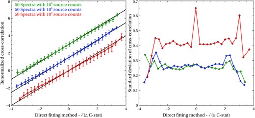
Comparison between the direct fitting and the cross-correlation methods. A totsl of 150 spectra of three different data qualities (shown here in different colours according to the legend) were simulated and searched with both methods. The left subplot shows the comparison of two equivalent quantities from both methods for all searched parameters from all the simulations. The blue and green groups were offset vertically for a better visualisation, the black lines correspond to y = x functions for the corresponding data groups. The original clouds of points were adaptively binned horizontally so that each point has Gaussian statistics (minimum 25 data per point) and so that they sample the horizontal range by roughly 0.25. The uncertainty of each bin is the standard deviation of cross-correlation values within it. The right subplot shows the standard deviation of the cross-correlation distribution across the horizontal (direct fitting method) range.
We also checked the cross-correlation search results from the 150 synthetic simulations for the presence of false detections due to any possible RGS instrumental features (e.g. many detections at the same wavelengths in the simulated spectra). We did not find any such features.
4.3 Example analysis: NGC 1313 X-1
We show an example analysis of the archetypal ULX NGC 1313 X-1 with the cross-correlation method as this ULX exhibits a known ultrafast wind (Pinto et al. 2016, 2020b).
We present the analysis of Stack1, which is the original data set where Pinto et al. (2016) discovered the ionized outflow in absorption as well as ionized rest-frame emission. The EPIC pn and RGS data sets, reduced following Section B1 are fitted with the standard three-component ULX broad-band spectral continuum described in Section B2. We find a power-law slope of 2.18, the temperature of the cooler blackbody is 0.17 keV, and the temperature of the hotter blackbody is 3.39 keV. All three components are obscured by neutral absorption with a column of 2.18 × 1021 cm−2.
We generate the Gaussian spectral models with the different velocity widths (according to Section B4) in the useful wavelength range of 7–23 Å, which is not background-dominated. Then the source spectra are simulated using the continuum model and the same clean exposure of 287 ks as the real data set. Afterwards the models and the residuals are cross-correlated following Section B6. We derive the renormalized correlation, TS, and the STS for each wavelength bin of the searched range, and for each velocity width in our parameter grid. These quantities are shown in Fig. 2 alongside the raw RGS residuals. A comparison can be made with fig. 3 in Pinto et al. (2016). The differences between the results can be attributed to differences in the search methods used and in the chosen broad-band spectral continuum.

The cross-correlation search of Stack1 of NGC 1313 X-1 performed between 7 and 23 Å. The top subplot shows the (stacked and heavily overbinned) RGS residuals to the broad-band spectral continuum. The second subplot contains the single trial significance, the renormalized correlation is shown in the third subplot and the true significance is in the bottom subplot. Searches with different Gaussian velocity widths are in different colours (according to the plot key in the bottom subplot). The red horizontal lines in the second subplot show the minimum/maximum attainable single trial significance given the performed number of simulations (10 000).
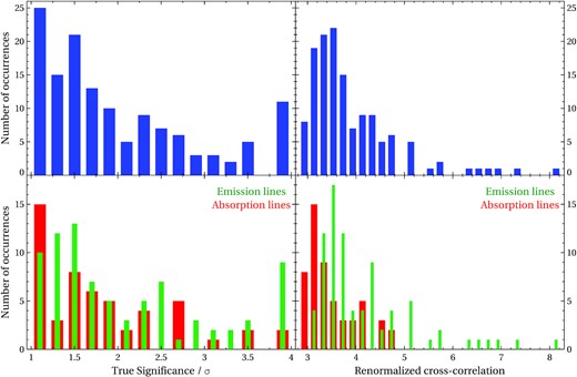
The histograms of true significances (left subplots) and renormalized cross-correlations (right subplots) of the detected lines. The top subplots show the total statistics for all lines, while the bottom subplots show the statistics for emission and absorption lines separately.
We immediately notice a strong absorption residual at 20 Å (interpreted as O VII absorption blueshifted by ∼0.1c). The STS plot shows that this residual is so strong that none of the 10 000 simulations produced a comparably strong residual at that specific wavelength, even though its TS is just below 3σ. This shows how important it is to account for the look-elsewhere effect for features not found at the rest-frame wavelengths of any expected transitions. There is also a broad absorption residual at 11–12 Å, which appears weak in the TS plot, however, a broader absorption feature (or multiple lines) would likely fit the residual better (and with a much higher significance). Pinto et al. (2016) show that this residual particularly stands out when a broader velocity width is used (10 000 km s−1). This is beyond the scope of this project, which focuses mainly on narrow line features.
Additionally, we also notice a number of emission features, especially at wavelengths of 12, 17, and 19 Å. These correspond to rest-frame emission from the ions of Ne X, Fe xvii, and O viii. Their minimum significances are between 1σ and 3σ, however, since they likely correspond to rest-frame emission, their real significance is more in line with the value of the renormalized cross-correlation or the STS.
We caution the reader against direct comparisons of this Gaussian line scan with more in-depth searches using physical plasma models that prove that the ionized outflow detection in NGC 1313 X-1 is highly significant at 4σ–5σ (Pinto et al. 2020b). The plasma models aggregate significance by combining the fit improvement statistics of multiple spectral lines at once, which all agree with the same outflow scenario. Therefore while a single feature might appear insignificant by itself, a combination of lines at different wavelengths, all fitted with the same physical model can result in a strong detection of an outflow (which is the case here).
The information about the individual spectral features is condensed in the ULX line catalogue where we only list the significantly detected lines (>1σ TS). Table 2 reports an excerpt from the catalogue showing just the search of this data set, containing the strongest features.
Excerpt from the ULX catalogue containing just the strongest lines detected in the Stack1 observations of NGC 1313 X-1. The 20-column catalogue table is split into four rows for display purposes. Each column is described in more detail in Appendix A.
| Object name | Approach | Wavelength | Energy | Turb. velocity |
|---|---|---|---|---|
| (Å) | (keV) | (km s−1) | ||
| NGC 1313X1 | Stack1 | 1.2260e+01 | 1.0113e+00 | 0.0000e+00 |
| NGC 1313X1 | Stack1 | 1.7110e+01 | 7.2463e-01 | 0.0000e+00 |
| NGC 1313X1 | Stack1 | 1.8100e+01 | 6.8500e-01 | 0.0000e+00 |
| NGC 1313X1 | Stack1 | 1.8940e+01 | 6.5462e-01 | 1.0000e+03 |
| NGC 1313X1 | Stack1 | 2.0090e+01 | 6.1715e-01 | 3.0000e+03 |
| True p-value | True signif. | Renorm. corr. | Single trial p-value | Single trial sig. |
| 1.5910e-01 | 1.4081e+00 | 3.4639e+00 | 8.1284e-04 | 3.3484e+00 |
| 1.7500e-02 | 2.3760e+00 | 4.1371e+00 | 2.0092e-04 | 3.7179e+00 |
| 2.4740e-01 | −1.1567e+00 | −3.1172e+00 | 1.4028e-03 | −3.1941e+00 |
| 2.2890e-01 | 1.2032e+00 | 3.3313e+00 | 1.6191e-03 | 3.1524e+00 |
| 6.0000e-03 | −2.7478e+00 | −4.0637e+00 | 1.9759e-04 | −3.7221e+00 |
| ΔC-stat | Photon flux | − | + | En. flux |
| ph cm−2 s−1 | ph cm−2 s−1 | ph cm−2 s−1 | erg cm−2 s−1 | |
| 1.0990e+01 | 3.0283e-06 | −9.7796e-07 | 1.0407e-06 | 4.9049e-15 |
| 1.4320e+01 | 2.1361e-06 | −6.4111e-07 | 6.6604e-07 | 2.4803e-15 |
| 1.1030e+01 | −2.0115e-06 | −5.5441e-07 | 5.7847e-07 | −2.2071e-15 |
| 1.0540e+01 | 2.7839e-06 | −8.8956e-07 | 9.7828e-07 | 2.9199e-15 |
| 1.4800e+01 | −6.0691e-06 | −1.5135e-06 | 1.5523e-06 | −6.0031e-15 |
| − | + | Equiv. width | − | + |
| erg cm−2 s−1 | erg cm−2 s−1 | keV | keV | keV |
| −1.5840e-15 | 1.6856e-15 | 5.9537e-03 | −2.0084e-03 | 2.1334e-03 |
| −7.4443e-16 | 7.7338e-16 | 3.6281e-03 | −1.1412e-03 | 1.1845e-03 |
| −6.0831e-16 | 6.3472e-16 | −2.9891e-03 | −8.6689e-04 | 9.0348e-04 |
| −9.3301e-16 | 1.0261e-15 | 4.2088e-03 | −1.4055e-03 | 1.5408e-03 |
| −1.4970e-15 | 1.5354e-15 | −1.0183e-02 | −2.6860e-03 | 2.7540e-03 |
4.4 The full sample
The final catalogue of the strongest detected features (with TS above 1σ) contains 135 spectral lines, of which 82 are emission and 53 are absorption lines.
We have obtained the true p-value for each line, i.e. the maximum false positive rate in case the feature is not located at a wavelength of any expected atomic transition (which includes the look-elsewhere effect). This means that we can directly calculate the maximum contamination rate of the catalogue – the probability that an average feature from the catalogue originates due to noise rather than due to a physical process. This percentage, obtained by summing all the individual line true p-values and dividing by the size of the catalogue is found to be 11 per cent. We find that the contamination fraction of emission features, 10 per cent (at most ∼8 fake emission features in the catalogue), is somewhat smaller than that of absorption features, which is 13 per cent (at most ∼7 fake absorption features in the catalogue). Assuming instead that all the emission features originate from rest-frame plasma (which might not be the case) reduces the contamination fraction of emission lines down to only 0.06 per cent (<<1 expected fake emission feature in the catalogue). This once again illustrates how important is the look-elsewhere effect in a blind search of a high-resolution data set.
To study the statistics of the detected lines, we created histograms of their significances. The TS and the renormalized cross-correlation distributions are shown in Fig. 3. The lower cut-off at TS of 1σ is imposed by our selection criteria. The peak of TSs near 4σ is due to the total number of simulations performed per object giving the maximum achievable significance (i.e. in a number of these cases, the ∼4σ significance quoted is actually a lower limit to the actual detection significance). We notice that many of the detected features apparently have quite low TSs between 1σ and 2σ. However, it is important to note that these are the absolute minimum significances of these features in the case that they are not located near an expected elemental transition (which many are expected to be). Even though the significances might seem low, the overall catalogue contamination fraction is not large at about 11 per cent. If we study the emission and absorption feature statistics separately (lower subplots in Fig. 3), we find their distributions are reasonably similar except for a higher abundance of lower significance absorption features, and a lack of very significant (∼4σ) absorption features.
5 DISCUSSION
In this work, we collected all suitable high-resolution XMM–Newton RGS data of ULXs and of two nearby super-Eddington pulsars and searched them for ionized plasma spectral features, both in absorption or emission. Collecting the 135 strongest line detections (with rigorously determined detection significances), we created the first catalogue of spectral lines in ULXs. Up to this point nothing was assumed about the origin and the emission/absorption process that produced these spectral features. In attempt to understand their physics, we plot the wavelengths of the significantly detected emission and absorption lines separately in two histograms, shown in Fig. 4.
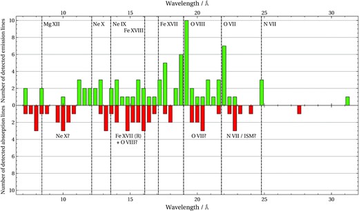
The histograms of the emission (green) and absorption (red) lines detected in the full sample versus their wavelength. The histograms are binned by 0.4 Å. Labels show the likely identification of the most abundant emission lines and the vertical dashed lines give the rest-frame wavelengths of these transitions. Considering the absorption lines are most likely Doppler-shifted, their preliminary identifications must be taken cautiously.
As expected, we find that many of the detected emission lines are grouped around known strong elemental transitions. This has been previously remarked by Pinto et al. (2016) and Kosec et al. (2018a) but using much smaller samples of ULXs and line detections. The most commonly observed features are the emission lines of O VII (rest-frame wavelength of the triplet around 22 Å) and O viii (19 Å). There is also strong evidence for Fe XVII/XVIII, the wavelengths of the strongest lines of its species are around 15–16 Å and then particularly around 17 Å. Another strongly detected element is Ne, represented by Ne IX (around 13.5 Å) and Ne X (12.1 Å). The range around 11–12 Å could also possibly contain the emission lines from rest-frame Fe XX-XXIV transitions. Finally, we also observe detections around the N VII transition (24.8 Å) and some evidence for the Mg XII transition at 8.4 Å.
The situation is completely different if we consider the absorption features. In general, we find that not many absorption lines occur at wavelengths with common occurrence of emission features (the rest-frame positions of strong elemental transitions). This is particularly true for the very common O VII, O viii, and Ne X features, although the Fe XVII/Fe XVIII region between 13 and 17 Å seems to be an exception with presence of both emission and absorption lines. The observed anticorrelation of occurrence of absorption and emission features is not surprising, considering that the absorption likely originates from a fast disc wind crossing our line of sight towards the central X-ray source. These winds have been shown to flow at large velocities (0.1–0.3c) in a few ULX (Pinto et al. 2016, 2017; Kosec et al. 2018b), hence the blueshifts of the absorption lines are considerable. If these winds indeed occur in most ULXs and with such typical velocities, we can tentatively guess the identification of the detected absorption residuals.
The absorption lines appear to be clustered into multiple groups. The group observed around 20 Å could originate from blueshifted O VII absorption (with velocities of ∼0.1c). The broad group seen between 14.5 and 17 Å could then be a blend of O viii and Fe XVII-XVIII absorption with velocities of 0.1–0.2c. The next strong group is at 9–11 Å and could originate from Doppler-shifted Ne X absorption (again shifted by ∼0.2c, with possible contribution from slower Fe XX-XXIV absorption). The groups around 8 and 13–14 Å could be imprinted by fast Fe XXIV and Fe XVII/XVIII ions, or by Mg XI/XII and Ne IX if the projected wind velocities are somewhat lower. Finally, we also observe a group of features between 22 and 24 Å. These could originate from blueshifted N VII absorption (at ≲0.1c), however this wavelength range also contains a number of low ionization O lines (e.g. O II and III at 23.4 and 23.0 Å, respectively) and dust absorption features (22.8–23.0 Å, e.g. Pinto et al. 2013) that could be imprinted on the ULX spectrum by the intervening interstellar medium (the continuum spectral model only accounts for the neutral gas).
We also compare the results of spectral searches of different sources. It is particularly interesting to compare the number of significantly detected lines versus the ULX data quality (RGS counts) and other properties such as its spectral hardness or its X-ray luminosity. ULXs show a large range of spectral hardnesses (Sutton, Roberts & Middleton 2013), thought to be related to their inclination angles and/or their mass accretion rates. The number of significantly detected features versus the quality of source spectra is shown in Fig. 5. Naturally, we find that better data quality on average results in more significant detections.
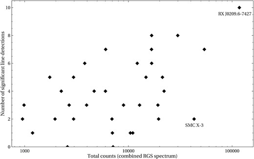
The number of significantly detected lines in each individual approach versus the number of net counts in its combined RGS spectrum. Labels show the super-Eddington pulsars in our sample. The remaining points all correspond to ULXs.
Importantly, we also find that spectrally harder ULXs show fewer detections than spectrally soft ULXs (Fig. 6, left subplot). The colour scheme in Fig. 6 shows the data quality (number of source counts in the combined RGS spectrum), and illustrates that even good quality RGS data sets (∼10 000 counts) of hard ULXs result in few line detections while much lower quality soft ULX data sets often show many more line detections. Similar results were previously presented in Kosec et al. (2018a) but using a much smaller sample of ULXs and a different analysis method. The Pearson correlation coefficient of the relationship between the number of line detections and the spectral hardness (the two super-Eddington pulsars excluded) is −0.67 with a false positive probability of 2.4 × 10⁻⁵, suggesting a highly significant anticorrelation. To show that this is not a data quality effect, we split the ULX-only sample by data quality into two groups. The higher data quality group gives a Pearson coefficient of −0.62 (p-value 9.1 × 10⁻³) and the lower data quality group a coefficient of −0.74 (p-value of 6.6 × 10⁻⁴).
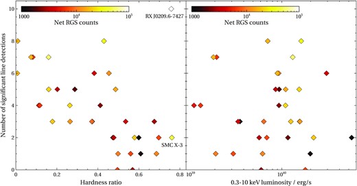
Left subplot: The number of significantly detected lines in each individual approach versus the spectral hardness of the source calculated from the broad-band spectral model such as H/(H+S), where H is the 2–10 keV de-absorbed luminosity and S the 0.3–2.0 keV de-absorbed luminosity. Right subplot: The number of significantly detected lines in each individual approach versus the de-absorbed 0.3–10 keV luminosity calculated from the broad-band spectral model. The colour scale in both subplots shows the total net counts in the combined RGS spectrum.
We also studied whether this anticorrelation holds for emission and absorption lines separately. Naturally, the statistics of the separate populations is much smaller and thus the trends are weaker. Importantly, we found that none of the two line populations show an equally strong trend as seen in the combined data set. This suggests that a similar anticorrelation is observed in both emission and absorption line populations. The Pearson correlation coefficients for these two populations (with the two super-Eddington pulsars excluded) are −0.56 (p-value 8.7 × 10⁻⁴) for emission lines and −0.59 (p-value 4.3 × 10⁻⁴) for absorption lines.
One of the leading scenarios explaining the difference between spectrally soft and hard ULXs suggests that soft ULXs are very similar objects to hard ULXs but observed from higher inclination angles. In that case, the hotter (and spectrally harder) central accretion flow regions are obscured from our view in soft ULXs by a geometrically thick super-Eddington accretion disc but directly visible in the hard ULXs. A schematic of this scenario is shown in fig. 13 of Pinto et al. (2017). The scenario can readily explain the lack of absorption features in hard ULXs since the ionized disc wind might not be crossing our line of sight in these sources at all. In fact, Pinto et al. (2020a) find a correlation between the projected velocity, the ionization parameter of the outflow and the hardness ratio of the ULX for the few sources in which fast winds were detected. This correlation was interpreted as an orientation effect.
However, to explain the lack of emission lines is more challenging. If the hardness is directly related to object inclination (and no other quantities), the emission line regions should be subject to the same spectral energy distribution (SED) in both hard and soft sources since their position with respect to the accretion flow should not change. Thus they should produce the same radiation output as they originate from optically thin plasma. At the same total luminosity the harder sources have less flux in the soft X-ray band where the lines are detected than the soft sources. The contrast between the lines and the continuum should then be even higher and they should be easier to detect in harder ULXs. Alternatively, the emission lines could be outshined in harder ULXs by the directly visible inner accretion flow regions (contributing also to soft flux), leading to lower line equivalent widths (and harder detectability) as suggested by Middleton et al. (2015) and Pinto et al. (2017). This, however, necessarily implies a higher X-ray luminosity but we find no correlation between the number of line detections and the ULX luminosity (Fig. 6, right). Hence, the lack of emission lines is difficult to reconcile unless they are obscured in hard ULXs, which seems unlikely. Perhaps, it suggests that other factors such as the mass accretion rate are more important drivers of ULX spectral hardness rather than their orientation towards us alone.
Therefore, the observed anticorrelation between the number of features and the source hardness suggests some difference between the plasma conditions or location in soft and hard ULXs. The difference in line detection rates could be due to the different SEDs of these two subclasses of ULXs. The harder SEDs of hard ULXs could ionize the plasma elements to higher ionization levels than the softer SEDs of soft ULXs, resulting in weaker line features that are much harder to detect (particularly in ULXs with poorer RGS data quality). Alternatively, if radiation line pressure contributes or drives the outflows, harder SEDs would result in less driving force and thus in lower mass outflow rates (although even soft ULX SEDs are quite hard for radiation line driving). Future ULX studies with instruments such as Athena achieving many more line detections (in much less exposure time), especially above 1 keV (from hotter plasma phases), will likely be able to explain this difference between soft and hard ULXs.
There may be alternative explanations for the observed anticorrelation between the number of detected lines and ULX spectral hardness, and the lack of correlation with luminosity, beyond different inclinations and mass accretion rates. Two black hole ULXs, despite similar luminosities, could have different fractions of mass lost to outflows and energy lost to advection/photon trapping, leading to very different line spectra and hardnesses (due to down-scattering in the wind). Similarly, two neutron star ULXs with comparable luminosities could have different spins and magnetic field strengths, resulting in different magnetosphere sizes. Assuming the outflow is produced in a supercritical part of the disc beyond the magnetosphere, different magnetosphere size would lead to very different outflow properties. Smaller magnetosphere would likely result in more massive and faster outflows due to the supercritical disc extending more inwards. The different magnetosphere size would also lead to different spectral hardnesses considering the accretion disc is spectrally softer than the accretion column and more mass in outflows would likely result in more photon down-scattering.
So far, we mostly studied the sample of ULXs and super-Eddington pulsars as whole. From Fig. 6 (left), where the two pulsars are specifically labelled, we can see that they are the hardest sources in our sample. SMC X-3 only shows two significant line detections, in line with the trend seen in spectrally harder ULXs. On the contrary, RX J0209.6-7427 shows 10 line detections despite its hardness (the most per source in the whole sample), however, we note that its RGS data set is by far the highest quality data set in the sample with over 100 000 combined source counts (see Fig. 5). The statistics of detected line wavelengths are very limited, but we observe strong similarities with the full sample. Most emission lines are seen near strong rest-frame transitions (O viii, O VII and N VII, however the higher ionization lines such as Fe XVII and Ne X are missing), while most absorption lines are avoiding the expected transition wavelengths.
A single spectral feature (especially if it has a 1σ–2σ minimum significance) detected alone in a ULX spectrum is not equivalent to an ionized outflow detection. However, if a single feature is detected, it is likely that any possible plasma/outflow might have also imprinted other spectral features, potentially weaker and thus not selected by our procedure. In Fig. 5, we can see that there are four cases of a single significant line detection in a data set.
The natural next step is therefore to try to describe multiple spectral lines at once, using a physical plasma model (ionized emission or absorption). The plasma model can be generated for a broad range of plausible physical parameters such as the ionization parameter, systematic velocity, and velocity width, and the ULX spectra can be searched for its spectral signatures. The significance of any plasma detection will be a combination of the significances of the individual spectral lines. Even features weak individually can add up to a significant detection because the TS of a detection rises very steeply with increasing fit improvement ΔC-stat (or Δχ2). For example, in the case of NGC 300 ULX-1 (Kosec et al. 2018b) where a fast ionized outflow was detected with a TS of around 3.7σ, its strongest single spectral line (blueshifted O viii line) was found in this work to be only significant at 1.3σ alone (TS). Applying a physical model can thus reveal much weaker plasma signatures. On the other hand, an important disadvantage of searching the ULX spectra with these models is that this is necessarily a much more model-dependent approach than using simple Gaussian line models to describe the residuals. Alternatively, a simpler and less model-dependent compromise could be to adopt a combination of a small number of Gaussian lines – e.g. an emission line triplet (to describe O VII or Ne IX emission), or to use a P-Cygni shape (to describe a possible wide angle outflow contributing both to ionized emission and absorption).
It is possible to extend the current cross-correlation analysis to physical plasma models or more complex spectral shapes by replacing the spectral model generation step in Section B4. This extension is beyond the scope of this paper and will be addressed in future work.
6 CONCLUSIONS
We systematically studied all suitable high-resolution soft X-ray spectra of Ultraluminous X-ray sources and searched them for plasma signatures in emission or in absorption. To assign the true false positive probability to each of the detected features (including the look-elsewhere effect), we developed a new, computationally affordable method of searching for Gaussian features in X-ray spectra. The method is based on cross-correlation, and it is more than 10 000 times faster than the previous approaches based on automated direct spectral fitting. By collecting all the detected spectral features, we created the first catalogue of spectral line detections in the soft X-ray spectra of ULXs. The catalogue contains 135 candidate lines (82 emission, 53 absorption lines) with a contamination fraction due to noise of at most 11 per cent. Over 90 per cent of studied sources show at least one spectral line, and roughly a third of the sources at least five line detections.
Most detected emission features are located at wavelengths corresponding to known transitions of ionic species of O, Fe, Ne, N, and Mg. On the other hand, the absorption lines generally appear to avoid these wavelengths and instead appear to be distributed between them. This is in agreement with a hypothesis that the emission lines originate in low-velocity material, while the absorption lines originate in fast disc winds crossing our line of sight with velocities of 0.1–0.3c. If this is indeed the case, such ultrafast outflows are common in many ULXs alongside with lower velocity wind components producing the observed emission lines.
We also find that spectrally harder ULXs show fewer spectral line detections than spectrally soft ULXs. This indicates a difference in the ULX accretion geometry/viewing angle which cannot be explained purely by their different orientation towards the observer. The difference could be due to overionization of the ionic species by the harder SEDs of harder ULXs. Further observations with high-resolution X-ray instruments are necessary to increase the line statistics and understand the observed trend. At the same time, no correlation is observed between the number of line detections and the ULX X-ray luminosity.
Further research directions for the systematic approach pioneered in this work include the extension of the cross-correlation method. It could be extended to allow the automated search for physical plasma models in X-ray spectra. Another option is the application of the search method to other X-ray sources such as AGN and Galactic X-ray binaries. The method could in particular be applied for automated search of ultrafast outflows in the X-ray spectra of AGN.
SUPPORTING INFORMATION
suppl_data
Please note: Oxford University Press is not responsible for the content or functionality of any supporting materials supplied by the authors. Any queries (other than missing material) should be directed to the corresponding author for the article.
ACKNOWLEDGEMENTS
We are grateful to the anonymous referee for useful comments that improved the quality of the manuscript. PK acknowledges support from the European Space Agency. Support for this work was provided by the National Aeronautics and Space Administration through the Smithsonian Astrophysical Observatory (SAO) contract SV3-73016 to MIT for Support of the Chandra X-Ray Center and Science Instruments. CSR thanks the UK Science and Technology Facilities Council for support under the New Applicant grant ST/R000867/1, and the European Research Council for support under the European Union’s Horizon 2020 research and innovation programme (grant 834203). This work is based on observations obtained with XMM–Newton, an ESA science mission funded by ESA Member States and USA (NASA). This research has used the NASA/IPAC Extragalactic Database, which is funded by the NASA and operated by the California Institute of Technology.
DATA AVAILABILITY
All of the data underlying this article are publicly available from ESA’s XMM–Newton Science Archive1 and NASA’s HEASARC archive.2
Footnotes
REFERENCES
APPENDIX A: CATALOGUE STRUCTURE
The catalogue is in the form of a single table saved in the ASCII format. The table contains all the strongest emission and absorption features as selected from the raw results, which have a TS of at least 1σ. The table contains 135 rows and 20 columns plus a two-row header with column descriptions and physical units. Each row corresponds to a single line feature detected in a specific ULX. The columns contain the following. The first column contains the source name and the second the observation or observations in which the line feature was found. Column 3 lists the wavelength of the feature (in Å), column 4 the energy (in keV) and column 5 the velocity width (in km s−1) at which the line shows the strongest cross-correlation. Columns 6 and 7 contain the true false positive rate and significance of the feature. Column 8 lists the renormalized correlation of the feature, and columns 9 and 10 show its single trial false positive rate and the STS. Column 11 lists the ΔC-stat fit improvement value obtained upon directly fitting the feature in the spex fitting package. Columns 12–14 contain the line photon flux (in photons cm−2 s−1) and its lower and upper errorbars. Columns 15–17 contain the line energy flux (in erg cm−2 s−1) with lower and upper errorbars, respectively. Finally, columns 18–20 contain the line equivalent width (in keV) and its lower and upper errorbars.
We note that wherever the TS, the renormalized cross-correlation and the STS are negative in the catalogue, this simply indicates that the feature found is an absorption line. Positive values of those quantities indicate that the feature is an emission line. We also note that all of the uncertainties in the catalogue are stated at 1σ confidence.
APPENDIX B: STEP-BY-STEP EXPLANATION OF THE CROSS-CORRELATION METHOD
Analysis parts B1–B5 as well as part B7 are run mostly as bash scripts (because bash offers automated access to spex) but also involve manual fitting within spex (part B2). Part B6 is written in python.
B1 Data reduction
In the first step, all XMM–Newton data are reduced. The data were downloaded from the XMM–Newton Science Archive and reduced using the standard sas v17.0.0 pipeline, CALDB as of 2020 June. We reduced XMM–Newton RGS and EPIC pn data.
The RGS data were reduced using the rgsproc procedure, and filtered for any flaring events with a threshold of 0.25 cts s−1 in each of the detectors. They were binned by a factor of 3 directly within the spex fitting package to oversample the instrumental resolution by roughly a factor of 3. They were used in the wavelength range which was not dominated by background flux. The exact range depended on the source and background fluxes of each object but often the range between 7 and 20 or 26 Å was chosen. For approaches using multiple stacked observations, we stacked the RGS 1 and RGS 2 spectra separately, producing two independent spectra to be fitted simultaneously.
The EPIC pn data were used to model the broad-band (0.3–10 keV) ULX spectrum correctly. The data were reduced using the epproc procedure and filtered for any background flares with a threshold of 0.5 cts s−1. The images of the pn exposures were prepared with the evselect procedure. The source regions were circles, usually with a radius of 35 arcsec. However, this was not always possible due to contamination by nearby X-ray sources. In those cases a smaller source region radius (20 or 25 arcsec) was chosen. The background regions were of polygon shape, at least 110 arcsec away from the main source to avoid the wings of its point spread function, at the same time avoiding any other bright X-ray sources. The background regions were located on the same chip as the source and were as large as possible to maximize the background statistics, whilst still located in the Copper hole on the EPIC pn chip (Freyberg et al. 2004; Carter & Read 2007). The background-subtracted pn spectra were binned to at least 25 counts per bin (achieving Gaussian statistics) and to oversample the real spectral resolution by a factor of at most 3 using the specgroup procedure. They were used in the 0.3–10 keV spectral range, but ignored in the wavelength range where RGS data were available. This way the spectral fit was not driven by EPIC pn data with much higher statistics (but much poorer spectral resolution) in the useful RGS range.
B2 Continuum modelling
After data reduction, the source spectra (RGS1 + RGS2 + pn) were fitted with a broad-band continuum spectral model, to locate any potential residuals around the best-fitting X-ray continuum. The fitting was performed manually within the spex fitting package to avoid mis-fitting of the spectra.
We chose to use a phenomenological ULX spectral model, previously employed also by Kosec et al. (2018a). The model is composed of three emission components: a power law, a blackbody modified by coherent Compton scattering and a standard blackbody. The power-law component (pow in spex) represents emission from the innermost regions of the ULX accretion flow – from an optically thin corona in the case of a black hole accretor or from an accretion column in the case of a neutron star accretor. The second component, a blackbody modified by coherent Compton scattering (mbb in spex), with temperatures of 1–3 keV represents X-ray emission from the hot, inner accretion disc of the ULX. The third component, a standard blackbody (bb in spex) with lower (0.1–0.2 keV) temperatures represents either emission from the colder, outer accretion disc, or emission from an optically thick outflow launched by the super-Eddington accretion flow. Finally, the spectrum is affected by interstellar absorption along our line of sight towards the ULX. Neutral gas in both our Galaxy and in the ULX host galaxy can contribute to this absorption, and thus the absorber column density was left free to vary in our continuum fits.
The spectral model is motivated by the physical picture outlined above. Nevertheless, the best-fitting model parameters such as the blackbody temperatures and power-law slopes should be interpreted with caution as our models do not include description of the hard X-ray ULX emission (above 10 keV). The absence of hard X-ray data (by only including XMM–Newton spectra) could lead to systematic uncertainties on these continuum parameters. However, ultimately, the model is primarily designed to ensure a good phenomenological fit to the XMM–Newton continuum, and therefore should not be compared too seriously to the results from truly broad-band spectral fits which include the NuSTAR hard X-ray coverage.
The broad-band model fits the spectra of most ULXs very well with no obvious broad systematic residuals. Considering the ULX spectral hardness is calculated from the model luminosity (rather than X-ray flux), a model-dependent hardness ratio uncertainty could be introduced, if the model over or underpredicts the true neutral absorption column density. This would result in systematically over or underpredicted ULX hardness ratios (with no effect on the actual Gaussian search). However, we do not estimate the errors introduced through the model choice to be too serious and prefer this approach to calculating spectral hardness from raw fluxes, which ignore the various ULX column densities altogether.
In a minority of cases, the soft standard blackbody was not required for an acceptable fit. In those cases only the power law and the modified blackbody was used. This was particularly the case in those ULXs where the neutral absorption column was high (above 1022 cm−2).
B3 Pre-filtering the data
In the third step of the routine, we identified any low quality wavelength bins in the source spectrum and discarded them. In the current version of the cross-correlation method, we simply discarded any wavelength bins where the continuum spectral model value was abnormally high – usually these defect bins appear as a delta function in the spectral plot and are too narrow to be real lines in the continuum spectral model. They correspond to bad pixels on the RGS detectors. The filtering threshold was chosen manually upon inspection of the spectrum, and the identified wavelength bin positions were discarded automatically in further analysis. The testing of our method showed that not excluding these defects could affect the correct renormalization of the cross-correlations later in the analysis.
B4 Generating real and simulated residual spectra
After the low-quality bins were identified, the residual spectrum of the source around the best-fitting broad-band model was generated and saved. The Y-axis of the spectrum was in units of Photons m−2 s−1 Å−1, i.e. the residuals were saved in physical units. The exact Y-axis unit is unimportant but it must be a unit of flux rather than a ratio to model values or a ratio to error bars, otherwise the cross-correlation method would find peaks in the data quality space rather than fitting physical shapes.
The source spectrum was simulated with the simulate command within spex, assuming just the best-fitting broad-band continuum affected by Poisson noise, and assuming the exposure of the same length as the real spectrum (and with the same background level). The residuals of each simulation to the continuum model were saved similarly as done with the real data set. We neglect the uncertainties on the assumed broad-band continuum, however, these are unlikely to be significant considering the continuum is anchored by the high quality EPIC spectrum and is smooth and featureless.
The simulations were repeated as many times as required. In this study we performed 10 000 simulations for each source, which means that we can probe significances of up to about 4σ. We found that the best computational performance was achieved if the simulated residuals were stored in files by large blocks, for example, by storing 5000 individual simulations in a single file. This grouping results in a large table where the columns are individual simulations and the rows correspond to the same wavelength bins. As we are searching through data from two individual instruments (RGS 1 and RGS 2), each column begins with data from RGS1, followed by data from RGS2.
B5 Generating spectral models
The next step was to generate the spectral models to cross-correlate with the real and simulated data sets. First, the real data set was loaded into spex (RGS1 and RGS2 simultaneously) and the low quality wavelength bins were ignored, thus ensuring the wavelength bins and range were identical to the ones in the real and simulated data. Then, the spectral model to be searched for was loaded. In this work, we simply loaded a Gaussian line as the spectral model. The Gaussian had a predefined line width (calculated from the velocity width |$v$| we were searching for) and a predefined wavelength λ. The velocity width of the line is related to its full width at half-maximum (FWHM) through the following equation: FWHM = 2.355|$v$|λ/c. The value of its normalization was positive (it was an emission line), but its exact value was unimportant (considering the cross-correlations were later renormalized) and was kept constant for all spectral searches in this study. The spectral model was saved, and then the parameters of the Gaussian were varied according to a grid of parameters we were searching over, saving the model at each step. Each saved spectral model was a column with as many rows as there were wavelength bins in our RGS 1 and RGS 2 data sets. The spectral models for RGS1 and RGS2 were similar but not exactly the same (they have different defect pixels and chips, different chip gap wavelengths and slightly different effective areas).
We searched the full usable RGS wavelength range (the exact range depended on each specific source) with a precision of 0.01 Å, which slightly oversampled the instrumental resolution of RGS. We also probed a range of different velocity widths of plasma producing the spectral lines. The line width was calculated from the appropriate velocity width at each wavelength. As a compromise between sampling and computational expense, we searched 12 different velocity widths: 0, 250, 500, 750, 1000, 1250, 1500, 2000, 2500, 3000, 4000, and 5000 km s−1. We did not search for lines with widths too large to avoid interpreting broad continuum model residuals, likely originating in imperfect broad-band modelling, as absorption or emission lines. For each source data set, the spectral models were stored in 12 individual table files, one for each value of velocity width.
B6 Cross-correlation
After the real/simulated data and the spectral model files were obtained, the main cross-correlation part of the routine was performed. First, all the spectral model file tables were loaded into RAM memory as a 3D array.
Secondly, the real source data set was cross-correlated with the all spectral model files, file-by-file, and column-by-column in each model file. We used the correlate function within the numpy package in python programming language. Cross-correlation is a symmetrical process and therefore even though our model files were composed of emission Gaussian lines, we were searching simultaneously for emission (positive correlations) and absorption (negative correlations) features.
Afterwards, the simulated data sets were loaded block-by-block and cross-correlated with all the spectral model files in the same fashion as done with the real data, and their raw correlations were saved. We calculated the number of each positive and negative correlation simulations (in each parameter bin), as well as the sums of squares of all positive and negative correlations (independently) in each bin.
Once the normalization factors were calculated from the raw correlations of all 10 000 simulated data sets, the raw correlations of the real data set were reloaded into memory and normalized by the Rλ, |$v$| + (positive raw correlations) and Rλ, |$v$| − (negative raw correlations) factors. We repeated the same procedure for the simulated data sets, block by block.
B7 Collecting results
As the normalized cross-correlations were being saved, they were ordered by value within their wavelength/velocity width bins. The normalized cross-correlation value of the real data set at each parameter bin was compared with these ordered lists and thus we obtained the p-value of each bin in the real data set (i.e. what fraction of simulated data sets showed stronger correlation or anticorrelation compared with the real data set). This value gives the STS of each bin.
At the same time, we saved the strongest correlation and anticorrelation from each of the simulated data sets. At this stage we combined the results from all individual spectral model files, obtaining the strongest correlations and anticorrelations for each simulation, taking into account all the spectral model parameters searched. Afterwards, these two extreme values from each simulation were ordered and compared with the real data set. We thus obtained the true p-value of each cross-correlation in the real data – for each searched parameter bin in the real data we determined the fraction of simulated data sets showing a feature (anywhere within the searched parameter range) stronger than the real one. The true p-value (TS) therefore takes fully into account the look-elsewhere effect.
Given that we obtained the various significances for each wavelength bin in the real data set for each of the spectral model parameters (12 different velocity widths), this was a considerable amount of data which needed to be filtered. We filtered only the strongest spectral features, selecting any correlation peak with the TS higher than 1σ (true p-value lower than 33 per cent). In case a peak at a certain wavelength appeared in searches with different velocity widths, we chose just the velocity width with the highest normalized correlation.
Finally, we ran an automated routine that took the wavelengths and velocity widths of the selected peaks and fitted Gaussian lines with such properties to the source spectrum directly (in spex). From the direct fit, we recovered the statistical fit improvement upon adding the extra Gaussian to the broad-band continuum (the ΔC-stat value), as well as the photon and energy fluxes of the added line, and we calculated its equivalent width.
APPENDIX C: STATISTICS OF EACH SEARCHED DATA SET, WITH DETAILS OF INDIVIDUAL OBJECTS
Table C1 shows the clean RGS exposures and the net RGS counts for each approach of every object studied in this work. We also show the hardness ratio of each spectrum calculated from the broad-band spectral model such as H/(S+H), where H is the luminosity in the 2–10 keV energy band and S is the luminosity in the 0.3–2.0 keV band. The hardness ratio is calculated from absorption-corrected luminosities. Finally, the table also shows the number of significant line detections in each of the sources studied (for each approach).
Clean RGS exposures (per detector) and total RGS net counts (both detectors combined) for each approach on every object in the ULX sample. The exposure column lists two exposures (RGS 1/RGS 2) in cases where they differed significantly. The fourth column lists the hardness ratios of each spectrum determined from the broad-band spectral continuum fits. The final three columns show the number of significantly detected line features – the total number and the number of emission and absorption features, respectively.
| Object name | Approach | Clean exposure | RGS net counts | Hardness ratio | Detected lines | Emission | Absorption |
|---|---|---|---|---|---|---|---|
| (ks) | H/(S+H) | ||||||
| Circinus ULX-5 | 0701981001 | 48 | 1191 | 0.609 | 1 | 1 | 0 |
| Circinus ULX-5 | 0824450301 | 118 | 2685 | 0.675 | 3 | 2 | 1 |
| Holmberg II X-1 | 0200470101 | 56 | 12818 | 0.264 | 3 | 2 | 1 |
| Holmberg II X-1 | Stack1 | 17 | 2253 | 0.412 | 4 | 1 | 3 |
| Holmberg II X-1 | FullStack | 137 | 22088 | 0.263 | 4 | 4 | 0 |
| Holmberg IX X-1 | 0200980101 | 96 | 7115 | 0.496 | 0 | 0 | 0 |
| Holmberg IX X-1 | FullStack | 181 | 19555 | 0.579 | 2 | 2 | 0 |
| IC 342 X-1 | Stack1 | 87 | 1744 | 0.288 | 5 | 4 | 1 |
| M33 X-8 | FullStack | 26/33 | 10448 | 0.498 | 1 | 1 | 0 |
| NGC 1313 X-1 | Stack1 | 287 | 14778 | 0.486 | 5 | 3 | 2 |
| NGC 1313 X-1 | Stack2 | 406 | 29922 | 0.430 | 8 | 4 | 4 |
| NGC 1313 X-1 | Stack3 | 304 | 12177 | 0.454 | 6 | 4 | 2 |
| NGC 1313 X-2 | Stack1 | 76 | 1962 | 0.473 | 2 | 1 | 1 |
| NGC 1313 X-2 | Stack2 | 102 | 986 | 0.372 | 3 | 1 | 2 |
| NGC 1313 X-2 | FullStack | 177 | 2962 | 0.478 | 2 | 1 | 1 |
| NGC 247 ULX | Stack1 | 706/718 | 16757 | 0.0088 | 8 | 5 | 3 |
| NGC 247 ULX | Stack2 | 706/718 | 16757 | 0.0074 | 6 | 3 | 3 |
| NGC 300 ULX-1 | 0791010101 | 134 | 7013 | 0.560 | 1 | 1 | 0 |
| NGC 300 ULX-1 | 0791010301 | 77 | 3954 | 0.535 | 3 | 2 | 1 |
| NGC 4190 ULX-1 | FullStack | 43 | 2585 | 0.569 | 0 | 0 | 0 |
| NGC 4559 X-7 | 0842340201 | 72 | 3793 | 0.382 | 6 | 3 | 3 |
| NGC 5204 X-1 | FullStack | 162 | 8975 | 0.371 | 3 | 3 | 0 |
| NGC 5408 X-1 | Stack1 | 237 | 21294 | 0.160 | 5 | 3 | 2 |
| NGC 5408 X-1 | Stack2 | 238 | 19261 | 0.179 | 3 | 1 | 2 |
| NGC 5408 X-1 | FullStack | 664 | 53986 | 0.160 | 7 | 4 | 3 |
| NGC 55 ULX | 0655050101 | 120 | 6038 | 0.083 | 7 | 5 | 2 |
| NGC 55 ULX | 0824570101 | 135 | 4677 | 0.112 | 4 | 3 | 1 |
| NGC 55 ULX | 0864810101 | 130 | 6009 | 0.117 | 4 | 1 | 3 |
| NGC 55 ULX | FullStack | 385 | 16713 | 0.074 | 7 | 5 | 2 |
| NGC 5643 X-1 | 0744050101 | 109 | 953 | 0.600 | 2 | 2 | 0 |
| NGC 6946 X-1 | 0691570101 | 110 | 2959 | 0.202 | 5 | 3 | 2 |
| NGC 7793 P13 | Stack1 | 226 | 6945 | 0.697 | 2 | 2 | 0 |
| NGC 7793 P13 | FullStack | 385/389 | 11025 | 0.686 | 1 | 0 | 1 |
| RX J0209.6-7427 | 0854590501 | 12 | 117516 | 0.758 | 10 | 3 | 7 |
| SMC X-3 | 0793182901 | 32 | 43018 | 0.761 | 2 | 2 | 0 |
Below, we list basic details of the individual objects studied in this work. We explain the approaches applied in their analysis as well as list the best-fitting broad-band continua.
In general, we analysed all the individual XMM–Newton observations that are of high enough data quality. Many sources have individual observations with quality lower than the 1000 count threshold, for which reason we also made stacks of all the available XMM–Newton observations (called FullStack) for those objects. We did not create a FullStack if the individual observations were of very high quality (around 15 000 counts of more). We also created smaller stacks of observations performed very close in time to each other, thus minimizing any long-term variations in the spectral lines. Finally, we did not create a FullStack spectrum if the increase in counts compared with the best data set of the same object was less than 50 per cent since the statistics would just be dominated by the best data set.
C1 Circinus ULX-5
There are two XMM–Newton observations of this ULX that are of high enough quality for our analysis (Walton et al. 2013). We analyse them individually. We do not attempt to stack them into a single data set because the gained data quality would not be sufficient (<50 per cent gain compared with the best individual observation), especially considering that the observations occurred many years apart.
Applying the three-component spectral model, we found that the soft blackbody was not required for a reasonable fit. This could be due to high neutral absorption column, found to be in the range of (6.3 − 7.4) × 1021 cm−2. The best-fitting power-law slope was found to be 1.9 and 2.5. The hot blackbody temperature was 2.0–2.2 keV.
C2 Holmberg II X-1
Holmberg II X-1 is a very well studied, nearby and bright ULX, with a wealth of XMM–Newton observations. We used three different approaches to study it: we searched the individual observation 0200470101 that is of high data quality (first studied by Goad et al. 2006). Secondly, Stack1 consists of two observations taken close in time to each other. Finally, we also examined the stacked spectrum from all the XMM–Newton observations.
The best-fitting broad-band continuum consists of a power law with a slope of Γ ∼ 2−2.5 (depending on the data set used), and two blackbodies with temperatures of 0.15–0.16 and 1.0–1.9 keV. The neutral absorption column density was 0.9–1.3 × 1021 cm−2.
C3 Holmberg IX X-1
Holmberg IX X-1 is another well-studied ULX, spectrally much harder than Holmberg II X-1. We chose two approaches to study it, following Kosec et al. (2018a). We analysed the long observation 0200980101 individually, and also stacked all the XMM–Newton observations.
All three spectral components were required for a good fit. We found a power-law slope of 2.0−2.6, and blackbody temperatures of 0.10–0.11 and 2.9–3.7 keV. The best-fitting neutral absorption column was 2.0–2.5 × 1021 cm−2.
C4 IC 342 X-1
There were two XMM–Newton observations well aligned for an RGS analysis of IC 342 X-1, and in both cases the source spectrum could be partially contaminated by another nearby X-ray source. As the observations individually were not of high enough quality, we stacked them into a single data set.
The three-component broad-band fit of this data set resulted in a power-law slope of 2.8, blackbody temperatures of 0.13 and 3.6 keV and a neutral absorption column 1.0 × 1022 cm−2.
C5 M33 X-8
M33 X-8 is the nearest extragalactic ULX but also the least luminous ULX in our sample. We stacked all four well-aligned XMM–Newton observations of the source into a single data set that is of good enough quality for our analysis.
Using the three-component spectral fit, we found a power-law slope of 1.9, and blackbody temperatures of 0.17 and 1.3 keV, obscured by a neutral column 1.2 × 1021 cm−2.
C6 NGC 1313 X-1
NGC 1313 X-1 is one of the best-studied ULXs with many long XMM–Newton observations. We split these observations into three stacks based on the NGC 1313 X-1 X-ray flux and spectral shape, following the strategy of Pinto et al. (2020b). We do not attempt to stack all of the individual observations into a single data set as the three stacks each result in data sets with excellent data quality.
The three-component model was required for an acceptable fit. We find power-law slopes in the range of 2.0−2.4, blackbody temperatures of 0.17–0.51 and 2.5–3.4 keV, and a neutral obscurer column of 2.2−2.5 × 1021 cm−2.
C7 NGC 1313 X-2
NGC 1313 X-2 has been extensively studied as part of the XMM–Newton campaigns on the brighter ULX in its host galaxy, X-1. However, most of the observations are not aligned well for an RGS analysis. We stacked all the available early observations (carried out between 2003 and 2005) into a single data set named Stack1. Stack2 consists of two observations 0764770101 and 0764770401 that were performed close to each other. Finally, we also stacked all the available data (FullStack).
The best-fitting three-component continuum resulted into power-law slopes of 2.0−2.3, blackbody temperatures of 0.11–0.17 and 1.9–2.4 keV and neutral absorption columns of 2.4–3.4 × 1021 cm−2.
C8 NGC 247 ULX
NGC 247 ULX is a very soft ULX that has recently been covered by a deep XMM–Newton campaign of eight long observations. Considering that these observations occurred close to each other and that the flux of the ULX is quite low, we stacked all of these spectra into a single data set.
Initially, we fitted the standard three-component spectral model. We found that only a single blackbody model was required. The power-law slope was very steep with Γ ∼ 4.2, the blackbody temperature was 0.13 keV and the neutral absorber column density was 3.9 × 1021 cm−2. This best-fitting continuum is analysed in the approach Stack1. However, upon inspection of the results, we found a very strong positive residual around 1 keV which strongly influenced the line search in this region. For this reason, we tried a second broad-band continuum, including a broad Gaussian line in this region to remove the very large effect of the 1 keV residual and hopefully reveal weaker spectral residuals in this band. The addition of the 1 keV Gaussian was highly significant with ΔC-stat∼100. The best-fitting produces a power law with a slope of 4.4, a blackbody with temperature 0.12 keV, a Gaussian with energy 0.92 keV and width 0.17 keV, all obscured by a neutral column of 4.0 × 1021 cm−2.
C9 NGC 300 ULX-1
NGC 300 ULX-1 is a ULX pulsar (Carpano et al. 2018) with two long XMM–Newton observations performed close to each other (0791010101 and 0791010301). We analysed these separately as Kosec et al. (2018b) showed a variation in the spectral residuals between the two observations as well as due to their individually high RGS counts.
All three spectral components were required for a good fit. We found a photon index of Γ ∼ 3.0−3.3, blackbody temperatures 0.25–0.30 and 2.9 keV and a neutral absorption column of 1.3–1.6 × 1021 cm−2.
C10 NGC 4190 ULX-1
There are four well-aligned XMM–Newton observations of this source, however, they are all individually of insufficient data quality, hence we stacked them into a single data set.
The continuum parameters recovered were as follows: power-law slope equal to 1.1, blackbody temperatures 0.13 and 1.7 keV and a neutral absorber column 1.7 × 1021 cm−2.
C11 NGC 4559 X-7
There is only one XMM–Newton observation of sufficient quality of this object, which we analysed here.
The best-fitting model required all three components and resulted in the following best-fitting parameters: power-law slope 2.1, blackbody temperatures 0.15 and 1.5 keV, and a neutral absorption column 1.6 × 1021 cm−2.
C12 NGC 5204 X-1
NGC 5204 X-1 has been observed many times by XMM–Newton but all the individual observations were rather short. We therefore stacked all of the individual observations into a single data set, following Kosec et al. (2018a).
The best-fitting continuum components consisted of a power law with a slope of 2.3, two blackbodies with temperatures of 0.2 and 2.0 keV and a neutral absorber with a column density of 8 × 1020 cm−2.
C13 NGC 5408 X-1
NGC 5408 X-1 has been observed many times by XMM–Newton with deep exposures. Two of these campaigns resulted in observations being performed close to each other. We therefore created two data set stacks (Stack1 and Stack2) from these campaigns. Additionally, we also created a stack of all the data sets that further increased the data quality but especially also included two other long observations not present in Stack1 and Stack2. Unfortunately, the orientation of the observations is such that another X-ray source is near the RGS source extraction region, and thus the ULX spectra could be partially contaminated. However, the EPIC data of the contaminating source show it is fainter and its spectra are much cleaner (featureless) than those of the ULX.
The best-fitting spectral model was as follows: a power law with a slope of 2.7−2.8, two blackbodies with temperatures of 0.14 keV and 1.2–1.4 keV, and a neutral absorber with a column of 1.0–1.2 × 1021 cm−2.
C14 NGC 55 ULX
NGC 55 ULX is a well-studied soft ULX that has recently been covered by three deep XMM–Newton observations. We were able to analyse all of them individually. We also decided to create a stacked spectrum (FullStack), which resulted in further increase in data quality to bring out any weaker spectral features that are not time variable.
All three spectral components were required for an acceptable fit. We found power-law slopes in the range of 2.6−3.5, blackbody temperatures of 0.15–0.17 and 0.64–0.70 keV. The neutral absorption column was around 2.3–3.1 × 1021 cm−2.
C15 NGC 5643 X-1
We analysed the only long observation of this distant ULX that is right on the border of our data quality cut.
We found that all three components were required. The power-law slope found was 1.6, and the blackbody temperatures were 0.16 and 1.8 keV, obscured by a neutral column of 1.8 × 1021 cm−2.
C16 NGC 6946 X-1
There are several XMM–Newton observations of this well-studied ULX. However, only one (0691570101) was found to be of high enough quality to analyse in this work.
The best-fitting continuum had a power-law slope of 2.4, blackbody temperatures of 0.17 and 1.5 keV, and a neutral absorber column density of 2.9 × 1021 cm−2.
C17 NGC 7793 P13
NGC 7793 P13 is an extremely well-studied pulsating ULX that has been observed many times by XMM–Newton. However, most of these observations were rather short and thus did not collect the required 1000 counts in the RGS detectors. Thus, we had to resort to stacking multiple observations. We created a single stack (FullStack) containing all the XMM–Newton observations of P13. Additionally, we also created another stack (Stack1) containing only the observations that occurred close to each other in 2017.
All three components were necessary for a good spectral fit. The best-fitting power-law slope was 2.8−2.9, and the blackbody temperatures were 0.22 and 3.5 keV, with a neutral absorption column density of 1.5 × 1021 cm−2.
C18 RX J0209.6-7427
RX J0209.6-7427 (Vasilopoulos et al. 2020) is an accreting pulsar in the SMC that has recently gone into a luminous outburst. Considering the mass of the neutron star is tightly constrained and the X-ray luminosity was around 1039 erg s−1, we know that the accretion rate of the object was highly super-Eddington during this event and thus we included it in this study of supercritical accretion. We use the only XMM–Newton observation of this object. Due to the low distance of the object and its luminosity this is a very high quality data set.
Considering the object belongs to a different class, its broad-band spectrum somewhat differs from the average ULX spectrum. Instead of the usual three-component model, we use a model composed of the following components. First, a Comptonisation component (comt in spex) with a plasma temperature of 3.1 keV, a seed photon temperature of 0.05 keV, and an optical density of τ ∼ 10. A simple power law is not a good description of the broad-band 0.3–10 keV spectrum due to its strong curvature towards the higher end of this energy range but a comt component results in a very good fit (see e.g. Kosec et al. 2020a, for its application in the study of the X-ray pulsar Hercules X-1). Secondly, we use a soft blackbody with a temperature of 0.13 keV and finally a broad Gaussian feature with an energy of 0.98 keV and a width of 0.27 keV. Using these components, absorbed by a neutral column of 5.8 × 1020 cm−2, resulted in a reasonable phenomenological fit, particularly in the RGS energy band.
C19 SMC X-3
SMC X-3 (Koliopanos & Vasilopoulos 2018) is another X-ray pulsar located in the SMC that is known to enter super-Eddington outbursts occasionally. XMM–Newton observed it during the latest outburst in 2016, and we analysed the observation (0793182901) in this work.
We employed a similar model to RX J0209.6-7427. We recovered the Comptonisation component plasma temperature of 3.7 keV, a photon seed temperature of 0.13 keV, an optical depth of 8.9 and a soft blackbody temperature of 0.13 keV. A broad ∼1 keV Gaussian feature was not necessary to obtain a good fit in this source. The neutral absorber column density was 1.9 × 1021 cm−2.
