


ABSTRACT
We describe and test the fiducial covariance matrix model for the combined two-point function analysis of the Dark Energy Survey Year 3 (DES-Y3) data set. Using a variety of new ansatzes for covariance modelling and testing, we validate the assumptions and approximations of this model. These include the assumption of Gaussian likelihood, the trispectrum contribution to the covariance, the impact of evaluating the model at a wrong set of parameters, the impact of masking and survey geometry, deviations from Poissonian shot noise, galaxy weighting schemes, and other sub-dominant effects. We find that our covariance model is robust and that its approximations have little impact on goodness of fit and parameter estimation. The largest impact on best-fitting figure-of-merit arises from the so-called fsky approximation for dealing with finite survey area, which on average increases the χ2 between maximum posterior model and measurement by |$3.7{{\ \rm per\ cent}}$| (Δχ2 ≈ 18.9). Standard methods to go beyond this approximation fail for DES-Y3, but we derive an approximate scheme to deal with these features. For parameter estimation, our ignorance of the exact parameters at which to evaluate our covariance model causes the dominant effect. We find that it increases the scatter of maximum posterior values for Ωm and σ8 by about |$3{{\ \rm per\ cent}}$| and for the dark energy equation-of-state parameter by about |$5{{\ \rm per\ cent}}$|.
1 INTRODUCTION
Our understanding of the Universe has become much more accurate in the past decades due to a massive amount of observational data collected through different probes, such as the cosmic microwave background (CMB; see e.g. Planck Collaboration VI 2020), big bang nucleosynthesis (see e.g. Fields et al. 2020), Type Ia supernovae (see e.g. Riess 2017; Smith et al. 2020), number counts of clusters of galaxies (see e.g. Mantz et al. 2014; Costanzi et al. 2019; Abbott et al. 2020), the correlation of galaxy positions, and that of their measured shape (see e.g. Abbott et al. 2018; Heymans et al. 2020). From the study of that data, a standard cosmological model has emerged characterized by a small number of parameters (see e.g. Frieman, Turner & Huterer 2008; Peebles 2012; Blandford et al. 2020). Current spectroscopic and photometric surveys of galaxies such as the Extended Baryon Oscillation Spectroscopic Survey1 and earlier phases of the Sloan Digital Sky Survey, the Hyper Suprime-Cam Subaru Strategic Program,2 the Kilo-Degree Survey (KiDS3), and the Dark Energy Survey (DES4) have become instrumental in testing this standard model at a new front: the growth of density perturbations in the late-time Universe. Also, future surveys, such as the Dark Energy Spectroscopic Instrument,5 the Vera Rubin Observatory Legacy Survey of Space and Time,6 Euclid,7 and the Nancy Grace Roman Space Telescope,8 will push this test to a precision exceeding that provided by other cosmological probes.
An important part of this program is the DES, a state-of-the-art galaxy survey that completed its 6-yr observational campaign in 2019 January (Diehl et al. 2019) collecting data on position, colour, and shape for more than 300 million galaxies. This makes DES the most sensitive and comprehensive photometric galaxy survey ever performed. The main cosmological analyses of the first year (Y1) of DES data have been concluded (Abbott et al. 2018, 2019b) and analyses of the first 3 yr of data (Y3) are under way. The study of the large-scale structure (LSS) of the Universe based on the DES-Y3 data set has the potential to become the most stringent test of our understanding of cosmological physics to date.
To achieve this goal, the DES team is comparing different theoretical models characterized by a range of cosmological parameters to the measured statistics of the LSS in order to determine the model and range of parameters that are in best agreement with the data. The statistics of the LSS considered in the main DES-Y3 analysis are two-point correlation functions of the galaxy density field (galaxy clustering), the weak gravitational lensing field (cosmic shear), and the cross-correlation functions between these fields (galaxy–galaxy lensing) in real space and measured in different redshift bins. These three types of two-point correlation functions are combined into one data vector – the so-called 3×2pt data vector.
A key ingredient in analysing these statistics is a model for the likelihood of a cosmological model given the measured correlation functions. Under the assumption of Gaussian statistical uncertainties (which is to be validated), this likelihood is completely characterized by the covariance matrix that describes how correlated the uncertainties of different data points in the 3×2pt data vector are. Validating the quality of the covariance model for the DES-Y3 two-point analyses is the main focus of this paper.
There are several methods to estimate covariance matrices that can roughly be divided into four main categories: covariance estimation from the data itself (e.g. through jackknife or sub-sampling methods; cf. Norberg et al. 2009; Friedrich et al. 2016), covariance estimation from a suite of simulations (e.g. Hartlap, Simon & Schneider 2007; Dodelson & Schneider 2013; Taylor, Joachimi & Kitching 2013; Percival et al. 2014; Taylor & Joachimi 2014; Joachimi 2017; Sellentin & Heavens 2017; Avila et al. 2018; Shirasaki et al. 2019), theoretical covariance modelling (e.g. Schneider et al. 2002; Eifler, Schneider & Hartlap 2009; Krause et al. 2017), or hybrid methods combining both simulations and theoretical covariance models (e.g. Pope & Szapudi 2008; Friedrich & Eifler 2018; Hall & Taylor 2019).
For the DES-Y3 3×2pt analysis, we adopt a theoretical covariance model as our fiducial covariance matrix. This fiducial covariance model is based on a halo model and includes a dominant Gaussian component, a non-Gaussian component (trispectrum and supersample covariance), redshift space distortions (RSDs), curved sky formalism, finite angular bin width, non-Limber computation for the clustering part, Gaussian shape noise, Poissonian shot noise, and fsky approximation to treat the finite DES-Y3 survey footprint (although taking into account the exact survey geometry when computing sampling noise contributions to the covariance). In order to assess the accuracy of that model, we study the impact of several approximations and assumptions that go into it (and into two-point function covariance models in general):
the Gaussian likelihood assumption, i.e. whether knowledge of the covariance is sufficient to calculate the likelihood;
robustness with respect to the modelling of the non-Gaussian covariance contributions, i.e. contributions from the trispectrum and supersample covariance;
treatment of the fact that two-point functions are measured in finite angular bins;
cosmology dependence of the covariance model;
random point shot noise;
the assumption of Poissonian shot noise;
survey geometry and the fsky approximation;
other covariance modelling details such as flat sky versus curved sky calculations, Limber approximation, and RSDs.
We generate different types of mock data and/or analytical estimates to determine how each of these effects impacts the quality of the fit between measurements of the 3×2pt data vector and maximum posterior models (quantified by the distribution of χ2 between the two). We also show how they impact cosmological parameter constraints derived from measurements of the 3×2pt data vector. For most of these tests, we employ a linearized Gaussian likelihood framework that allows us to analytically quantify the impact of covariance errors on the χ2 distribution and parameter constraints. This is complemented by a set of lognormal simulations and importance sampling techniques to quickly assess large numbers of mock (non-linear) likelihood analyses.
This paper is part of a larger release of scientific results from year-3 data of the DES and our analysis is informed by the (in some cases preliminary) analysis choices of the other DES-Y3 studies. In addition to carving out the most stringent constraints on cosmological parameters from late-time two-point statistics of galaxy density and cosmic shear yet, the year-3 analysis of the DES collaboration is introducing and testing numerous methodological innovations that pave the way for future experiments. Details of the DESY3 galaxy catalogues and the photometric estimation of their redshift distribution are presented by Sevilla-Noarbe et al. (2020), Hartley et al. (2020), Everett et al. (2020), Myles et al. (2021), Gatti et al. (2020a), Cawthon et al. (2020), Buchs et al. (2019), and Cordero et al. (2020). The measurements of galaxy shapes and the calibration of these measurements for the purpose of cosmic weak gravitational lensing analyses are detailed by Gatti et al. (2020b), Jarvis et al. (2020), and MacCrann et al. (2020). Krause et al. (2021) develop and test the theoretical modelling pipeline of the DES-Y3 3×2pt analysis, Pandey et al. (2021) outline how galaxy bias is incorporated in this pipeline, DeRose et al. (2020) validate this pipeline with the help of simulated data, and Muir et al. (2020) describe how we have blinded our analysis to focus our efforts on model-independent validation criteria and reduce the chance for confirmation bias. The DESY3 methodology to sample high-dimensional likelihoods and to characterize external and internal tensions is outlined by Lemos et al. (2021) and Doux et al. (2020). Measurements of cosmic shear two-point correlation functions and analyses thereof are presented by Amon et al. (2021) and Secco et al. (2021), the measurement and analysis of galaxy clustering wo-point statistics are carried out by Rodríguez-Monroy et al. (2021), and two-point cross-correlations between galaxy density and cosmic shear (galaxy–galaxy lensing) are measured and analysed by Prat et al. (2021), with additional analyses of lensing magnification and shear ratios carried out by Elvin-Poole et al., (in preparation) and Sánchez et al. (2021) and results for an alternative lens galaxy sample presented by Porredon et al. (2020) and Porredon et al., (2021). Finally, in DES Collaboration (2020) we present our cosmological analysis of the full 3×2pt data vector.
Our paper is structured as follows. We start by presenting a discussion of our validation strategy in Section 2, where we also summarize our main findings before plunging into the details in the remaining of the paper. In Section 3, we review the modelling and structure of the 3×2pt data vector. Section 4 describes our fiducial covariance model as well as two alternatives to it that are used to validate several modelling assumptions. In Section 5, we describe our linearized likelihood formalism and derive analytically how different covariance matrices impact parameter constraints and maximum posterior χ2 within that formalism (including the presence of nuisance parameters and allowing for Gaussian priors on these parameters). In Section 6, we present the details of each step in our validation strategy followed by a short Section 7 presenting a simple test to corroborate some of the results from the linearized framework. We conclude with a discussion of our results in Section 8. Seven appendices describe in more detail some results used in this work.
2 COVARIANCE VALIDATION STRATEGY AND SUMMARY OF THE RESULTS
How should one validate the quality of a covariance model (and the associated likelihood model) for the purpose of constraining cosmological model parameters from a measured statistic? A straightforward answer seems to be that one should run a large number of accurate cosmological simulations, then measure and analyse the statistic at hand in each of the simulated data sets, and test whether the true parameters of the simulations are located within the, say, |$68.3{{\ \rm per\ cent}}$| quantile of the inferred parameter constraints in |$68.3{{\ \rm per\ cent}}$| of the simulations. There are, however, at least two problems with such an approach.
Another more practical problem is the fact that it is not (yet) feasible to generate enough sufficiently accurate mock data sets to validate covariance matrices of large data vectors with high precision. We recall that for the DES-Y1 analysis, a total of 18 realistic simulated data sets were available to validate the inference pipeline (MacCrann et al. 2018). At the same time, the main reason why N-body simulations would be required to test the accuracy of covariance (and likelihood) models is to capture contributions to the covariance coming from the trispectrum (connected four-point function) of the cosmic density field. However, for DES-like analyses it has been shown that this contribution is negligible (see e.g. Krause et al. 2017; Barreira, Krause & Schmidt 2018). The reason for this is twofold: First, very small scales (where the trispectrum contribution to the covariance would matter most) are often cut off from analyses because on these scales already the modelling of the data vector, |$\boldsymbol{\xi }[\boldsymbol{\pi }]$|, is inaccurate. Secondly, on small scales the covariance matrix is often dominated by effects coming from sparse sampling such as shot noise and shape noise. These covariance contributions are typically easy to model (although one has to be careful when estimating effective number densities and shape-noise dispersions or when estimating the number of galaxy pairs in the presence of complex survey footprints; see Troxel et al. 2018a, b).
As a result of the above considerations, we base our covariance validation strategy mostly on the use of a linearized likelihood (where the model |$\boldsymbol{\xi }[\boldsymbol{\pi }]$| is linear in the parameters |$\boldsymbol{\pi }$|). In this framework, the Bayesian likelihood allows for an interpretation in terms of frequencies – both for total and marginalized constraints. Also, this allows us to perform large numbers of simulated likelihood analyses very efficiently, without the need to run computationally expensive Markov chain Monte Carlo (MCMC) codes. In addition, any leading-order deviation from a linearized likelihood will be next-to-leading order for the purpose of studying the impact of covariance errors (i.e. errors on errors) on our analysis.
Within the linearized likelihood formalism, we confirm the findings of Krause et al. (2017) and Barreira et al. (2018) for the DES-Y3 set-up: Both supersample covariance and trispectrum have a negligible impact on our analysis. This allows us to estimate the impact of other assumptions in our covariance and likelihood model either analytically or by the means of simplified mock data such as lognormal simulations (as opposed to full N-body simulations; cf. Section 4.3).
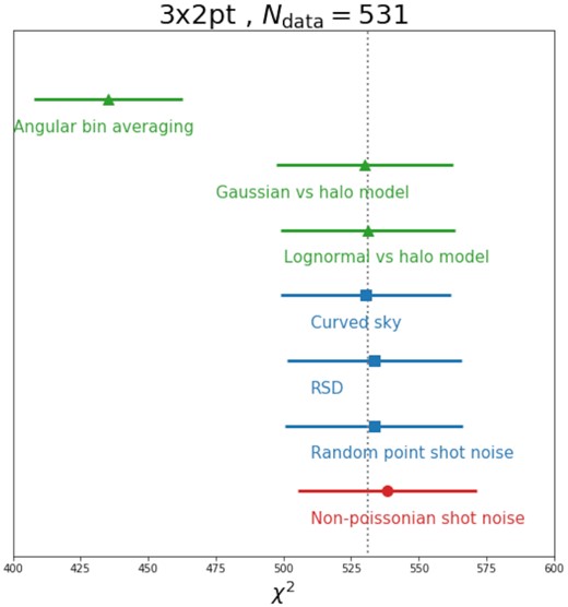
We summarize our main findings in Fig. 1 and Table 1 for the busy reader. For the combined data vector of the DES-Y3 two-point function analysis (the 3×2pt data vector; see details in Section 3), the left-hand panel of Fig. 1 shows the impact of different assumptions in our likelihood model on the mean and scatter of χ2 between maximum posterior model and measurements. To obtain the maximum posterior model, we are fitting for all the 28 parameters listed in Table 3 within the linearized likelihood framework described in Section 5.1. Since we assume Gaussian priors on 13 nuisance parameters, the effective number of parameters in that fit will be between 28 and 15. Within the linearized likelihood approach, we find that with a perfect covariance model the average χ2 is expected to be about 507.6; i.e. the effective number of degrees of freedom in the fit is Nparam,eff ≈ 23.4. The right-hand panel of Fig. 1 shows the equivalent results when cosmic shear correlation functions are excluded from the data vector (the 2×2pt data vector). The green points in both panels denote effects that have been already accounted for in the previous year-1 analysis of DES.
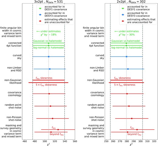
Impact of different covariance modelling choices on χ2 between measured 3×2pt (left-hand panel) and 2×2pt (right-hand panel) data vectors and maximum posterior models. The dashed vertical lines and error bars indicate the 1σ fluctuations expected in χ2. See the main text for details.
Summary of the impact of the different effects tested here on the distribution of χ2 between measurement and maximum posterior model, on the scatter |$\sigma [\hat{\pi }]$| of maximum posterior parameters |$\hat{\pi }$|, and on the standard deviations σπ on these parameters inferred from the likelihood. See the text for details.
| Effect | 〈χ2〉 | σ(χ2) | |$\sigma (\hat{\Omega }_\mathrm{ m})$| | |$\sigma _{\Omega _\mathrm{ m}}$| | |$\sigma (\hat{\sigma }_8)$| | |$\sigma _{\sigma _8}$| | |$\sigma (\hat{w})$| | σw |
|---|---|---|---|---|---|---|---|---|
| Fiducial | 507.6 | 31.8 | 0.0509 | 0.0509 | 0.0975 | 0.0975 | 0.244 | 0.244 |
| Angular bin width | 402.1 | 26.0 | +0.8 per cent | +7.4 per cent | +0.8 per cent | +8.3 per cent | +1.0 per cent | +7.4 per cent |
| Connected four-point function | 507.6 | 31.8 | +0.1 per cent | −0.8 per cent | +0.1 per cent | −0.9 per cent | +0.1 per cent | −0.8 per cent |
| Curved sky | 507.7 | 31.8 | +0.0 per cent | −0.0 per cent | +0.0 per cent | −0.0 per cent | +0.0 per cent | −0.0 per cent |
| Non-Limber and RSD | 511.4 | 32.1 | +0.1 per cent | −0.6 per cent | +0.1 per cent | −0.6 per cent | +0.3 per cent | −1.4 per cent |
| Non-Gauss. likelihood | – | 32.6 | +0.8 per cent (low) | – | +0.4 per cent (low) | – | +0.5 per cent (low) | – |
| −0.9 per cent (high) | −0.4 per cent (high) | +0.05 per cent (high) | ||||||
| Covariance cosmology | 508.6 | 32.4 | +2.9 per cent | +(0.1 ± 0.06) per cent | +2.8 per cent | +(0.1 ± 0.05) per cent | +4.7 per cent | +(0.1 ± 0.06) per cent |
| Random point shot noise | 511.3 | 32.0 | +0.0 per cent | −0.5 per cent | +0.0 per cent | −0.6 per cent | +0.0 per cent | −0.2 per cent |
| Non-Poisson shot noise | 515.0 | 32.3 | +0.0 per cent | −0.7 per cent | +0.0 per cent | −0.8 per cent | +0.0 per cent | −0.6 per cent |
| Masking and survey geometry | 526.5 | 33.8 | +0.6 per cent | −0.8 per cent | +0.7 per cent | −0.3 per cent | +0.3 per cent | −1.3 per cent |
What stands out in our analysis is the large effect of finite angular bin sizes on the cosmic variance and mixed terms of our covariance model (cf. Section 4 for this terminology, where we also show that it is unavoidable to take into account finite bin width in the pure shot noise and shape noise terms of the covariance). In DES-Y1, this has been dealt with in an approximate manner, by computing the covariance model for a very fine angular binning and then re-summing the matrix to obtain a coarser binning (Krause et al. 2017). This time we incorporate the exact treatment of finite angular bin size for all the three two-point functions into our fiducial covariance model (cf. Section 4). The blue points in Fig. 1 denote improvements that have been made in the year-3 analysis compared to the year-1 covariance model, and the red points are estimates of effects that are not taken into account in the fiducial DES-Y3 likelihood – either because they are negligible or because an exact treatment is unfeasible (cf. Section 6 for details). Adding these effects in quadrature, our results suggest that the maximum posterior χ2 of the DES-Y3 3×2pt analysis should be on average |$\approx 4{{\ \rm per\ cent}}$| (Δχ2 ≈ 20.3) higher than expected if the exact covariance matrix of our data vector was known.
Table 1 summarizes the offsets in χ2 displayed in the left-hand panel of Fig. 1 and also shows how parameter constraints based on the 3×2pt data vector are impacted by assumptions of our covariance and likelihood model. We distinguish two effects here: the scatter of a maximum posterior parameter π (which we denote by |$\sigma [\hat{\pi }]$|) and the width of posterior constraints inferred from our likelihood model (which we denote by σπ). For our tests of likelihood non-Gaussianity, we state the changes in the difference between the fiducial parameter values and the upper (high) and lower (low) boundaries of the 68.3 per cent quantile with respect to the standard deviation of the Gaussian likelihood. For our tests of the impact of covariance cosmology, we show the mean of all σπ obtained from our 100 different covariances and also indicate the scatter of these σπ values.
The effect that has the dominant impact on parameter constraints is that of evaluating the covariance model at a set of parameters that do not represent the exact cosmology of the Universe. When computing the covariance at 100 different cosmologies that were randomly drawn from a Monte Carlo Markov chain (run around a fiducial model data vector; see Section 6.8 for details), we find that the differences between these covariances introduce an additional scatter in maximum posterior parameter values. This scatter increases by about |$3{{\ \rm per\ cent}}$| for Ωm and σ8 and by about |$5{{\ \rm per\ cent}}$| for the dark energy equation-of-state parameter w. This increased scatter is in fact the dominant effect, since the width of the derived parameter constraints hardly changes between the different covariance matrices. Note especially that rerunning the analysis with a covariance updated to the best-fitting parameters does not mitigate this effect.
In Fig. 2, we take the two effects that had the largest impacts on χ2 and show the resulting mismatch between scatter of maximum posterior values and width of the inferred contours for a wider range of parameters. All of our results take into account marginalization over nuisance parameters (and all other parameters).
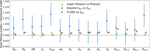
Impact of covariance errors on the ratio of the standard deviation of maximum posterior parameters to the width of the posterior derived from the erroneous covariance. Green triangles shot the effect caused by non-Poissonian shot-noise and orange circles show the effect caused by the fsky approximation (cf. Appendix C for our beyond-fsky treatment). These ratios have been calculated purely on the base of different analytic covariance models and within the linearized likelihood framework discussed in Section 5.1. We also show the ratio of maximum posterior parameter scatter observed from the 197 flask simulations to the statistical uncertainties expected from a lognormal covariance matrix matching the flask configuration. Within the statistical uncertainties, these ratios are consistent with 1.
Our reason for exclusively investigating the impact of covariance errors on χ2 and parameter constraints is that those are the two measures by which our final (on-shot) data analysis will be interpreted and judged.10 In the remainder of this paper, we detail how the above results were obtained.
3 THE 3×2-POINT DATA VECTOR
The combined 3×2pt data vector of the DES-Y3 analysis consists of measurements of the following two-point correlations:
the angular two-point correlation function w(θ) of galaxy density contrast measured for luminous red galaxies in five different redshift bins (see e.g. Rodríguez-Monroy et al. 2021; Cawthon et al. 2020, as well as other relevant references given in Section 1),
the auto- and cross-correlation functions ξ+(θ) and ξ−(θ) between the galaxy shapes of four redshift bins of source galaxies (see e.g. Amon et al. 2021; Gatti et al. 2020a; Myles et al. 2021; Secco et al. 2021),
the tangential shear γ(θ) imprinted on source galaxy shapes around positions of foreground redMaGiC galaxies (see e.g. Prat et al. 2021).
At the time of writing this paper, the exact choices for redshift intervals and angular bins considered for each two-point function are still being determined by a careful study of their impact on the robustness of DES-Y3 parameter constraints (DES Collaboration 2020; Krause et al. 2021). For the purposes of testing the modelling of the covariance matrix, we will use the most recent but possibly not final DES-Y3 analysis choices. We do not expect that our tests and conclusions will change in a significant manner with further updated analysis choices. We assume that each of the correlation functions is measured in 20 logarithmically spaced angular bins between θmin = 2.5 arcmin and θmax = 250 arcmin. Some of these bins in some of the measured two-point functions are being cut from the analysis to ensure unbiased cosmological results, resulting in a total of 531 data points when using the preliminary DES-Y3 scale cuts.
For most of our tests, we consider the 3×2pt data vector and its covariance matrix at the fiducial cosmology described in Section 5, where we also show the Gaussian priors assumed on some of these parameters when assessing the impact of covariance modelling on parameter constraints and maximum posterior χ2.
4 COVARIANCE MATRICES FOR THE 3 × 2PT DATA VECTOR
In the fiducial DES-Y3 analysis, we model all of these covariance contributions analytically. This fiducial model is described in Section 4.1. In Section 4.2, we describe an alternative model for the non-Gaussian covariance contributions that is used to test the robustness of our analysis with respect to the modelling of the trispectrum contribution. Finally, Section 4.3 describes a set of lognormal simulations (Xavier, Abdalla & Joachimi 2016) and the covariance matrix of the 3×2pt data vector estimated from them. These simulations also allow us to test the accuracy of our Gaussian likelihood assumption and the treatment of masking and finite survey area in our fiducial covariance model.
4.1 Fiducial DES-Y3 covariance
In our fiducial covariance matrix, we model the non-Gaussian covariance contributions |$\mathbf {C}_{\mathrm{nG}}$| and |$\mathbf {C}_{\mathrm{SSC}}$| using a halo model combined with leading-order perturbation theory to approximate the trispectrum of the cosmic density field and to compute the mode coupling between scales larger than the considered survey volume with scales inside that volume. These calculations are carried out using the CosmoCov code package (Fang et al. 2020a) based on the CosmoLike framework (Krause & Eifler 2017). Our modelling of these contributions has not changed with respect to the year-1 analysis of DES and we refer the reader to Krause et al. (2017) as well as to the CosmoLike papers for details. However, the modelling of the Gaussian contribution has changed as described in the following.
4.1.1 Gaussian covariance
Our modelling of the Gaussian covariance part has changed with respect to the year-1 analysis in the following ways:
we use (and present for the first time13) analytical expression for the angular bin averaging of the functions |$F^{AB}_\ell (\theta)$| (cf. equation 10) for all four types of two-point functions present in our data vector (see Section 6.3; this is especially relevant for the sampling-noise contribution to the covariance; cf. Troxel et al. 2018b);
we account for RSDs and also use a non-Limber calculation to obtain the galaxy–galaxy clustering power spectrum |$C_{\delta _\mathrm{ g }\delta _\mathrm{ g}}(\ell)$| (see Section 6.5);
we do not make use of the flat-sky approximation anymore (see Section 6.4).
4.2 Analytical lognormal covariance model
Our results are shown in Table 2, where we present the number density, galaxy bias (relevant for lenses only), shape-noise dispersion (per shear component; relevant for sources only), and the lognormal shift parameters obtained from the procedure described above. Note that for the source galaxy samples, the relevant line-of-sight projection kernel used to derive the shift parameter is the lensing kernel (and not the redshift distribution of the source galaxies). For the lens galaxies, all shift parameters come out to be >1. As a consequence, there will be pixels with negative density in our lognormal simulations. However, the fraction of such pixels is <0.01 for all runs and all bins and setting δg = −1 in these bins has an unnoticeable effect on the statistics measured in these maps (e.g. for bin 4, which is affected most, the standard deviation of δg changes by |$0.053{{\ \rm per\ cent}}$|). Note further that at the time of completing the simulation runs presented in Section 4.3, the DES-Y3 shear catalogue and redshift distribution were not finalized. As a consequence, the shape-noise dispersion values used for simulations differ from the values in this table. We display the projection kernels assumed for our analysis in Fig. 3.
Number density, galaxy bias (relevant for lenses only), shape-noise dispersion (per shear component; relevant for sources only), and the lognormal shift parameters obtained from the procedure described in Section 4.2.
| z-bin | ng (arcmin−2) | Bias | σϵ | Lognormal shift |
|---|---|---|---|---|
| Lenses 1 | 0.0221 | 1.7 | − | 1.089 |
| Lenses 2 | 0.0381 | 1.7 | − | 1.106 |
| Lenses 3 | 0.0583 | 1.7 | − | 1.047 |
| Lenses 4 | 0.0295 | 2.0 | − | 1.252 |
| Lenses 5 | 0.0251 | 2.0 | − | 1.177 |
| Sources 1 | 1.7971 | − | 0.2724 | 0.004 53 |
| Sources 2 | 1.5521 | − | 0.2724 | 0.008 85 |
| Sources 3 | 1.5967 | − | 0.2724 | 0.019 18 |
| Sources 4 | 1.0979 | − | 0.2724 | 0.032 87 |
4.3 Lognormal covariance from simulations
We also produce a test DES-Y3 covariance matrix from a set of simulations. We use the publicly available code flask (Full sky Lognormal Astro fields Simulation Kit; Xavier et al. 2016,14) to generate 800 DES-Y3 footprint sky maps of density, convergence, and shear healpix maps (Górski et al. 2005) with NSIDE = 8192, as well as galaxy positions catalogues, used to reproduce the DES-Y3 properties. flask is able to quickly produce tomographic correlated simulations of clustering and weak lensing lognormal fields based on the DES-Y3 lens and sources samples. The lognormal distribution of cosmological fields has been shown to be a good approximation (Coles & Jones 1991; Wild et al. 2005; Clerkin et al. 2017) but much less computationally expensive to generate than full N-body simulations.
As input for the simulations, we used a set of auto- and cross-correlated power spectrum and the lognormal field shift parameters. The theoretical input power spectrum was generated using CosmoLike, and the lognormal shifts are the ones listed in Table 2. In order to reproduce the properties of shear fields, we added the shape-noise term by sampling each pixel of the simulated maps to match the correspondent shape-noise dispersion σϵ and number density ng of the tomographic bin. At the time of completing the simulation runs, the DES-Y3 shear catalogue and redshift distribution were not finalized. For this reason, the values used in the simulations are slightly different from the values in Table 2. For the simulations, we set the number density for the five tomographic lens bins as 0.0227, 0.0392, 0.0583, 0.0451, and 0.0278 (arcmin−2). The shape-noise dispersion values for the four tomographic bins of sources were set to 0.270 49, 0.332 12, 0.325 37, and 0.350 37. The cosmology adopted for the theoretical power spectra is set as Ωm = 0.3, σ8 = 0.823 55, ns = 0.97, Ωb = 0.048, h0 = 0.69, and |$\Omega _\nu h_0^2 = 0.000\,83$|.
We use the publicly available code treecorr15 (Jarvis, Bernstein & Jain 2004) to measure the 3×2 point correlation measurements for 200 DES-Y3 realizations. For all measurements, we used 20 log-spaced angular separation bins on scales between 2.5 and 250 arcmin. We set the bin_slopTreeCorr parameter to zero, essentially setting all estimators to brute-force computation. In Fig. 4, we show the validation of the measurements comparing with the theoretical input.
We will use the flask covariance mainly to estimate the impact of the survey geometry.
4.4 Comparisons among covariances
Here, we present some comparisons between the different covariance matrices. In Fig. 5, we show the ratio of the diagonal elements of the different covariance matrices introduced in this section displaying both the variances of the measurements of ξ+(θ) of w(θ).
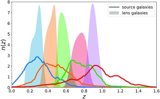
Redshift distributions of lens galaxies (shaded regions) and source galaxies (solid lines) in our fiducial test configuration.
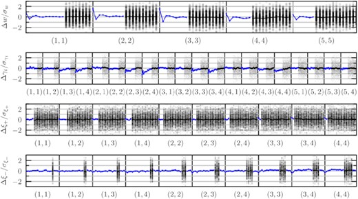
Validation of flask simulations. Each panel shows the absolute difference of three two-point correlations measured on flask realizations and the predicted correlation functions from input C(ℓ)s normalized to the statistical error given by the standard deviation along flask realizations (ΔX/σX, where X = w, γt, ξ+, ξ−). Grey dots are single realizations and blue dots its mean.
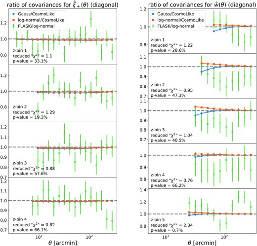
Ratio of the diagonal elements of the different covariance matrices introduced in this section with respect to each other. The left-hand panel compares the variances of measurements of ξ+(θ) while the right-hand panel compares the variances of measurements of w(θ). To give a sense of the goodness of fit between the covariance estimated from flask and our fiducial analytic matrix, we treat the diagonal elements of the flask covariance as a multivariate Gaussian whose covariance can be inferred from the properties of the Wishart distribution (Taylor et al. 2013). The low p-value for the highest redshift bin ofw(θ) most likely results from our incomplete treatment of the survey mask (cf. discussion in Section 6 and Appendix C).
In Fig. 6, we compare the covariance matrices obtained from the flask simulations and the analytical halo model covariance.
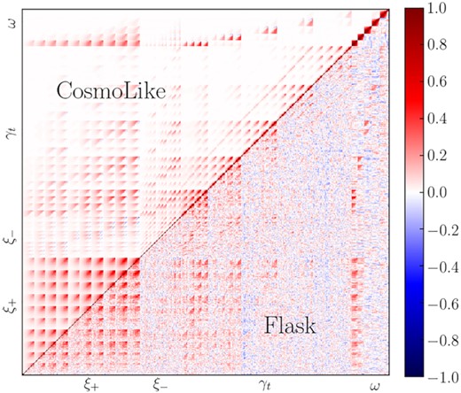
flask (lower diagonal) versus CosmoLike halo model (upper diagonal) correlation matrix.
5 IMPACT OF COVARIANCE ERRORS ON A LINEARIZED GAUSSIAN LIKELIHOOD
As discussed earlier, a full assessment of the impact of using different covariance matrices to parameter estimation becomes unfeasible due to the computational demand of running a large number of MCMC chains. Since the covariance matrices studied in this work differ by subdominant effects, we do not expect large modifications in the results of the estimation of the parameters. Therefore, we will bypass this difficulty by using a linearized approximation of the model data vector as a function of the parameters. The measured data are assumed to be a Gaussian multivariate variable characterized by a covariance matrix and a given prior matrix. This approach is called the Gaussian linear model (Seehars et al. 2014, 2016; Raveri & Hu 2019).
Within this approach, we study the following impacts of different covariances:
error in the parameter estimation, characterized by the width of the contours;
the scatter of the best-fitting (maximum posteriors) parameters;
change in the maximum posterior χ2 value;
error in the maximum posterior χ2 value.
In the remainder of this section, we detail this method.
5.1 Linearized likelihoods
Fiducial cosmology and standard deviation of Gaussian parameter priors used in our mock likelihood analyses. AIA, i is the intrinsic alignment amplitude in the i-th source redshift bin, mi is the multiplicative shear bias, and Δzs, i parametrizes systematic shifts in the photometric redshift distribution of that bin. Δzl, i parametrizes systematic shifts in the photometric redshift distribution of the i-th lens redshift bin. The Gaussian priors we choose for the parameters follow the analysis choices of Abbott et al. (2018) and we assume infinite flat priors for all other parameters.
| Parameter | Fiducial value | σprior |
|---|---|---|
| Cosmology | ||
| Ωm | 0.3 | – |
| σ8 | 0.823 55 | – |
| h100 | 0.69 | – |
| ns | 0.97 | – |
| w0 | −1 | – |
| Ωb | 0.048 | – |
| Ων | 0.001 743 | – |
| |$\Omega _\Lambda$| | 1 − Ωm − Ων | – |
| b1 | 1.7 | – |
| b2 | 1.7 | – |
| b3 | 1.7 | – |
| b4 | 2.0 | – |
| b5 | 2.0 | – |
| Δzl, 1 | 0.0 | 0.04 |
| Δzl, 2 | 0.0 | 0.04 |
| Δzl, 3 | 0.0 | 0.04 |
| Δzl, 4 | 0.0 | 0.04 |
| Δzl, 5 | 0.0 | 0.04 |
| Δzs, 1 | 0.0 | 0.08 |
| Δzs, 2 | 0.0 | 0.08 |
| Δzs, 3 | 0.0 | 0.08 |
| Δzs, 4 | 0.0 | 0.08 |
| AIA, 1 | 0.0 | – |
| AIA, 2 | 0.0 | – |
| AIA, 3 | 0.0 | – |
| AIA, 4 | 0.0 | – |
| m1 | 0.0 | 0.03 |
| m2 | 0.0 | 0.03 |
| m3 | 0.0 | 0.03 |
| m4 | 0.0 | 0.03 |
5.2 Impact on the width of the likelihood and scatter of best-fitting parameters
We can use the above findings to study the impact of different effects in covariance modelling on parameter constraints. If a covariance matrix |$\mathbf {C}_1$| contains a noise contribution that is missing in another covariance matrix |$\mathbf {C}_2$|, then we quantify the difference between these matrices by considering the following two effects:
- Width of likelihood contours: Denoting the Fisher matrices obtained from |$\mathbf {C}_1$| or |$\mathbf {C}_2$| as |$\mathbf {F}_1$| and |$\mathbf {F}_2$|, respectively, the widths of likelihood contours drawn from the different covariances are given byHence, if the difference |$\mathbf {C}_1-\mathbf {C}_2 = \mathbf {E}$| represents noise contributions missing from (or miss-estimated in |$\mathbf {C}_2$|), then a comparison of |$\mathbf {C}_{\boldsymbol{\pi }, \mathrm{like},\ 1}$| and |$\mathbf {C}_{\boldsymbol{\pi }, \mathrm{like},\ 2}$| quantifies the impact of this on the width of parameter contours.(35)$$\begin{eqnarray*} \mathbf {C}_{\boldsymbol{\pi }, \mathrm{like},\ 1} &=& (\mathbf {F}_1+\mathbf {P})^{-1}\nonumber \\ \mathbf {C}_{\boldsymbol{\pi }, \mathrm{like},\ 2} &=& (\mathbf {F}_2+\mathbf {P})^{-1}\ . \end{eqnarray*}$$
- Scatter in the centre of likelihood contours: If the data vector |$\boldsymbol{\hat{\xi }}$| had |$\mathbf {C}_1$| as its true covariance matrix but |$\mathbf {C}_2$| would be used to derive the maximum posterior parameters |$\boldsymbol{\pi }^{\mathrm{MP}}$| from it, then the maximum posterior parameter covariance would be given byIf the difference |$\mathbf {C}_1-\mathbf {C}_2 = \mathbf {E}$| represents noise contributions missing from (or miss-estimated in |$\mathbf {C}_2$|), then a comparison of |$\mathbf {C}_{\boldsymbol{\pi }, \mathrm{MP},\ 2}$| and |$\mathbf {C}_{\boldsymbol{\pi }, \mathrm{MP},\ 1} \equiv \mathbf {C}_{\boldsymbol{\pi }, \mathrm{like},\ 1}$| quantifies the impact of this on the scatter in the location of parameter contours.(36)$$\begin{eqnarray*} \left(\mathbf {C}_{\boldsymbol{\pi }, \mathrm{MP},\ 2}\right)_{\alpha \beta } &=&\ (\mathbf {F}_{\mathrm{2}}+\mathbf {P})^{-1}\ \mathbf {P}\ (\mathbf {F}_{\mathrm{2}}+\mathbf {P})^{-1} + \sum _{\kappa , \lambda } (\mathbf {F}_{\mathrm{2}} + \mathbf {P})_{\alpha \kappa }^{-1}\ (\mathbf {F}_{\mathrm{2}} + \mathbf {P})_{\lambda \beta }^{-1} \sum _{i,k} \partial _\kappa \xi _i\ \left(\mathbf {C}_{\mathrm{2}}^{-1\ }\mathbf {C}_{\mathrm{1}}\ \mathbf {C}_{\mathrm{2}}^{-1}\right)_{ik}\ \partial _\lambda \xi _k\ . \end{eqnarray*}$$
An inaccurate covariance model will in general have a different impact on the width and the location of parameter contours. Hence, in order to quantify the importance of different effects in covariance modelling for parameter estimation, we compare both the pair |$\mathbf {C}_{\boldsymbol{\pi }, \mathrm{like},\ 1} / \mathbf {C}_{\boldsymbol{\pi }, \mathrm{like},\ 2}$| and the pair |$\mathbf {C}_{\boldsymbol{\pi }, \mathrm{MP},\ 1} / \mathbf {C}_{\boldsymbol{\pi }, \mathrm{MP},\ 2}$|.
5.3 Distribution of χ2 when fitting for parameters
the true covariance |$\mathbf {C}$| of |$\boldsymbol{\hat{\xi }}$| is known;
no parameter priors are used when determining the best-fitting model |$\boldsymbol{\xi }_{\mathrm{MP}}$|;
the true expectation value |$\boldsymbol{\bar{\xi }} \equiv \langle \boldsymbol{\hat{\xi }}\rangle$| lies within our parameter space; i.e. there are parameters |$\boldsymbol{\pi }^{\mathrm{true}}$| such that |$\boldsymbol{\xi }(\boldsymbol{\pi }^{\mathrm{true}}) = \boldsymbol{\bar{\xi }}$|.
We will show that, as expected, in this case |$\hat{\chi }_{\mathrm{MP}}^2$| should follow a χ2 distribution with Ndata − Nparam degrees of freedom.
6 EXPLORING DIFFERENT EFFECTS IN THE COVARIANCE MODELLING
Our main goal is to study the impact of including different effects in the covariance modelling on the estimation of parameters. Several covariance matrices were generated and tested under different assumptions and approximations. The main results were already shown in Section 2. We now present the details of each step in the validation strategy that was outlined in Section 5.
6.1 Gaussian likelihood assumption
A basic assumption of our framework of testing different covariance matrices is that the likelihood function of the data is Gaussian. One simple reason of why the sampling distribution of the correlation functions cannot be an exact multivariate Gaussian is that this violates the positivity constraint of the power spectrum (Schneider & Hartlap 2009). There are also other reasons described below. The purpose of this subsection is to assess the impact of non-Gaussianity of the likelihood of two-point functions in the parameter estimation. In this sense, checking this basic assumption is a test of the whole framework and is different from the robustness tests for the covariance matrix modelling described in the remaining subsections of this section.
The impact of a non-Gaussian likelihood in parameter estimation of weak lensing correlation functions has been recently studied in Lin et al. (2020) where no significant biases were found in one-dimensional posteriors of Ωm and σ8 between the multivariate Gaussian likelihood model and more complex non-Gaussian likelihood models. Also, in Sellentin, Heymans & Harnois-Déraps (2018) the skewed distributions of weak lensing shear correlation functions are used to derive an analytical expression for a non-Gaussian likelihood.
In the top panel of Fig. 7, we show the impact of this non-Gaussianity on the distribution of maximum posterior χ2. For that figure, we generated 300 000 random realizations of our fiducial data vector from a multivariate Gaussian distribution, 300 000 random realizations of that data vector from a multivariate lognormal distribution, and 300 000 random realizations from another lognormal distribution, whose skewness in each data point was increased by a factor of 5. For each of these random realizations, we analytically determined the maximum posterior model within the linearized likelihood formalism of Section 5.1 and then computed the χ2 between that model and the random realization. The blue histogram in the top panel of Fig. 7 shows the distribution of these χ2 values for the Gaussian random realizations and the red histogram corresponds to the lognormal random realizations. The two histograms are almost identical. Hence, within the fsky approximation employed above non-Gaussianity in the likelihood does not seem to affect our analysis. Also, even in the extreme scenario of enhancing the skewness of the data vector by a factor of 5 (green histogram) the increase in the scatter of χ2 remains smaller than about |$3{{\ \rm per\ cent}}$| of the average χ2 – which still would not dominate over the other effects discussed in subsequent sections (cf. Fig. 1).
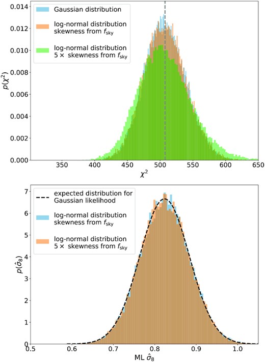
Top panel: Distribution of χ2 when drawing 3×2pt data vectors from a Gaussian distribution (blue histogram), from a shifted lognormal distribution where the skewness of each data point was computed in the fsky approximation (red histogram) and when assuming that the skewness of the data points is 5 times that of the fsky approximation (green histogram). Bottom panel: Distribution of maximum posterior σ8 when fitting the linearized model to Section 5.1 Gaussian realizations of our fiducial data vector, to lognormal realizations of our fiducial data vector (blue histogram), and to lognormal realizations with 5 times the skewness of the fsky approximation employed in Section 6.1 (orange histogram).
The impact of non-Gaussianity on the likelihood becomes even more negligible when directly considering the distribution of maximum posterior parameters. We demonstrate this in the bottom panel of Fig. 7 for the best-fitting values of σ8 but find similar results for our other key cosmological parameters Ωm and w0. Therefore, we conclude that it is safe to assume a Gaussian distribution for the statistical uncertainties of the DES-Y3 two-point function measurements.
6.2 Modelling of connected four-point function in covariance
The connected four-point contribution to the covariance is the part that is most challenging to model analytically (Schneider et al. 2002; Hilbert et al. 2011; Sato et al. 2011; Takada & Hu 2013). This contribution is most relevant at small scales and turns out to be a small one for current LSS analyses (Krause et al. 2017; Barreira et al. 2018). This is for two reasons: (1) such analyses typically cut away their smallest scales because of uncertainties in the modelling of their data vectors and (2) at small scales the covariance matrix is often dominated by shape noise and shot noise that are believed to be well understood.
We test whether the non-Gaussian covariance parts (by which we mean both the connected four-point function and supersample covariance) are a relevant contribution to our error budget by either
replacing the non-Gaussian contributions from the fiducial halo model with the lognormal covariance described in Section 4.2.
or setting it to zero, i.e. using only a Gaussian covariance matrix.
Fig. 1 and Table 1 show that neither of these changes has a significant impact on the distribution of χ2 and our parameter constraints. Assuming that our halo model and lognormal recipes do not underestimate the non-Gaussian covariance parts by orders of magnitude [see e.g. Sato et al. (2009) and Hilbert et al. (2011) for justifications of this assumption), this demonstrates that we are insensitive to the exact modelling of these contributions. At the same time, we want to stress that this finding holds for the specific scale cuts, redshift distributions, and tracer densities of the DESY3 3×2pt analysis and cannot necessarily be generalized to other analysis set-ups.
6.3 Exact angular bin averaging
The corresponding expressions for the galaxy–galaxy lensing correlation function γt(θ) and for the cosmic shear correlation functions ξ± are presented (together with derivations of all the bin averaged expressions) in Appendix B.
The impact of the exact angular bin averaging for the noise and mixed terms in the Gaussian part of the covariance matrix is included for all four types of two-point functions present in the DES-Y3 data vector and the DES-Y3 fiducial covariance.
6.4 Flat versus curved sky
For the Y1 analysis, it was shown that the flat-sky approximation was valid for the galaxy–galaxy shear and shear–shear two-point correlation function (Krause et al. 2017). In Y3, the fiducial covariance computes the full sky correlations; see equations (12) and (13). We show in Fig. 1 that the effect of including curved sky results has negligible impact on the χ2 distribution. Table 1 shows that this is also true for parameter constraints.
6.5 RSD and Limber approximation and RSD effects
The modelling of the angular power spectrum of two tracers involves a projection from the 3D power spectrum that requires integrals with integrands containing the product of two spherical Bessel functions, which are highly oscillatory. The inclusion of RSD effects in a simple linear modelling (Kaiser 1987) involves the computation of those integrals with derivatives of the Bessel functions. These integrals are notoriously difficult to perform numerically and it is usual to apply the so-called Limber approximation (Limber 1953; LoVerde & Afshordi 2008). An efficient computation of these integrals without resorting to the Limber approximation was recently implemented in the case of the angular power spectrum for galaxy clustering in Fang et al. (2020b). We use their approach to study the impact of taking into account both non-Limber computations and RSD effects in the covariance matrix. Fig. 1 and Table 1 show that not taking these effects into account leads to an increase in average χ2 of about |$0.5{{\ \rm per\ cent}}$| and an underestimation of uncertainties in key cosmological parameters by |$0.6{{\ \rm per\ cent}}$| to |$1.4{{\ \rm per\ cent}}$|.
6.6 Effect of the mask geometry
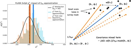
The impact of masking on the DES-Y3 covariance. The blue histogram in the right-hand panel shows the distribution of χ2 obtained from our flask data vectors when using the fsky approximation. We restrict this figure to the 2×2pt function part of the data vector since it is this part that suffers the most from masking effects (cf. Fig. 1). Ansatzes in the CMB literature (e.g. Efstathiou 2004) are not sufficient to correct for this, because the DES footprint has features down to very small scales. In the main text, we have motivated a possible way to correct for these small-scale masking features and the orange histogram in the left-hand panel shows that this ansatz indeed significantly improves the χ2 obtained from our flask measurements. The sketch in the right-hand panel visualizes how small-scale features in the mask lead to an overestimation in the covariance when using common ways to treat the impact of survey geometry on the two-point function covariance (see the main text for explanation).
The right-hand panel of Fig. 8 visualizes this for the mixed terms in the covariance, where one of the correlation functions ξac or ξbd is due to sampling noise such as shape noise or shot noise and is hence exactly proportional to a Dirac delta function. In that case, the integration is over pairs that share one end point. Now, the approximation made e.g. in Efstathiou (2004) or by our equation (68) assumes that also the correlation function between the other two end points effectively acts as a delta function with respect to the smallest scale features in the survey mask (cf. equation 70). We find that this is not the case for the DES-Y3 mask and that it contains features on all scales relevant to our analysis. However, as indicated in equation (71), one can approximately correct for this by multiplying the mixed terms in the covariance by the fraction fmask of the coarser survey geometry that is covered by small-scale holes in the mask. This can be considered a next-to-leading-order correction to our equation (68).
By applying equation (71) twice, one can see that the cosmic variance terms (terms where neither of the two-point functions ξac or ξbd are exactly proportional to delta functions) can be corrected by multiplication with |$f_{\mathrm{mask}}^2$|. To implement this correction in practice, we draw circles within the DES-Y3 survey footprint with radii ranging from 5 to 20 arcmin and measure the masking fraction in these circles. We find that this fraction is |${\approx} 90{{\ \rm per\ cent}}$| across the considered scales. Multiplying the mixed terms in the covariance by that fraction and the cosmic variance terms by the square of that fraction (together with using equation 68), we indeed find significant improvement of the maximum posterior χ2 obtained for the flask simulations – as is shown in the left-hand panel of Fig. 8 (as well as in Fig. 1).
In Fig. 9, we use our flask measurements together with the technique of precision matrix expansion (PME; from inverse covariance = precision matrix; Friedrich & Eifler 2018) and perform a consistency of the modelling ansatz described above by investigating the impact of masking on individual covariance terms. We find both with the PME methods and with our analytic ansatz that masking effects are most impactful in the covariance terms that depend on shape noise of the weak lensing source galaxies (i.e. in what we called mixed terms in Section 3). This also agrees with the findings of Joachimi et al. (2020) and it further motivates the modelling of masking effects that we have described here. Nevertheless, we do not elevate this modelling ansatz to our fiducial covariance model because its motivation remains rather heuristic. However, we consider it a realistic estimate for the error made by the fsky approximation and can hence use it to estimate the impact of that approximation on parameter constraints. In Fig. 2, we have already shown that this impact is below the |$1{{\ \rm per\ cent}}$| level; i.e. we underestimate the scatter of maximum posterior parameters by less than |$1{{\ \rm per\ cent}}$| when making the fsky approximation in our fiducial covariance model.
![The method of PME (Friedrich & Eifler 2018) allows us to estimate the impact of individual covariance terms on χ2 even when only few simulated measurements are available. The orange squares show the average χ2 between our flask measurements and their mean [re-scaled by a factor of Nflask/(Nflask − 1) to account for the correlation of individual measurements and mean] when using either no PME at all or when using PME estimates from shape-noise free sims or from the full sims. The blue dots show the corresponding χ2 values when using the heuristically motivated analytical treatment of masking and survey geometry presented in the main text. The grey dashed line represents the number of data points and should be the average χ2 if we had a perfect covariance model (note that for this comparison we have not performed any parameter fitting).](https://oup.silverchair-cdn.com/oup/backfile/Content_public/Journal/mnras/508/3/10.1093_mnras_stab2384/1/m_stab2384fig9.jpeg?Expires=1750212834&Signature=H9D5PHF94Lm8piafEfX4u3qLi2l2NS37feqQ-aZLZwrvmo3uL3-conCuHO-h0e1e07WRnWLHlpKdhqIE-~iBy9Z6eEEucUyAf2V47GRO-WbPKGS6lcg0qefJf00spXehdYyAoaPHNv6tNYs7axQOOBUr2igG1q73ogaVzqtbyvY7VXcQYEBuHajUnuLjPj18mTxUogwdsV2aVePq1PKEoiiA4F2y5tiBL7PJqYNiHCmkM096m03WKC5imlJWkQIVBU~ojGeL2ncRP2C~6BR~kUV8WcTxBRqUVGU5YCFgLxFNPMdYbrEvfhisbZzpd8x--QvfbxJ6ghG8Sbc07EbheQ__&Key-Pair-Id=APKAIE5G5CRDK6RD3PGA)
The method of PME (Friedrich & Eifler 2018) allows us to estimate the impact of individual covariance terms on χ2 even when only few simulated measurements are available. The orange squares show the average χ2 between our flask measurements and their mean [re-scaled by a factor of Nflask/(Nflask − 1) to account for the correlation of individual measurements and mean] when using either no PME at all or when using PME estimates from shape-noise free sims or from the full sims. The blue dots show the corresponding χ2 values when using the heuristically motivated analytical treatment of masking and survey geometry presented in the main text. The grey dashed line represents the number of data points and should be the average χ2 if we had a perfect covariance model (note that for this comparison we have not performed any parameter fitting).
Note that Kilbinger & Schneider (2004), Sato et al. (2011), Shirasaki et al. (2019), and Philcox & Eisenstein (2019) have devised and promoted an alternative method to correct for masking, which amounts to direct Monte Carlo integration of expressions like equation (69). Given the large area of DES-Y3 and its numerous combinations of redshift bins, we did not find this to be feasible.
6.7 Non-Poissonian shot noise
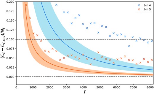
Measured ratio |$r_{\ell } = \frac{C_{\ell }-C_{\ell ,rnd}}{N_{\ell }}$| (crosses) compared to predicted contribution of the galaxy power spectra over the shot noise (solid line) for the fiducial parameters at Elvin-Poole et al. (2018) allowing for a 20 per cent uncertainty in the galaxy bias (shaded regions) for two redshift bins (bin 4 in blue and bin 5 in orange). Horizontal dashed lines are just to guide the eye. If the shot noise were to be completely Poissonian, the measured and predicted ratios would agree; however, we find an excess between |$2{{\ \rm per\ cent}}$| and |$6{{\ \rm per\ cent}}$|.
Best-fitting values of αn to correct for the excess shot noise with the DES-Y1 redmagic galaxies.
| Bin number | α |
|---|---|
| 1 | 1.042 ± 0.002 |
| 2 | 1.069 ± 0.003 |
| 3 | 1.072 ± 0.003 |
| 4 | 1.057 ± 0.003 |
| 5 | 1.021 ± 0.001 |
| Bin number | α |
|---|---|
| 1 | 1.042 ± 0.002 |
| 2 | 1.069 ± 0.003 |
| 3 | 1.072 ± 0.003 |
| 4 | 1.057 ± 0.003 |
| 5 | 1.021 ± 0.001 |
6.8 Cosmology dependence of the covariance model
In order to evaluate our covariance model, we choose a particular set of cosmological parameters. We do not vary these parameters when sampling our parameter posterior and this may impact the width of our parameter constraints (Hamimeche & Lewis 2008; Eifler et al. 2009; White & Padmanabhan 2015; Kalus, Percival & Samushia 2016). Our main reason for not sampling the covariance model along with the data model is that computing a covariance matrix is computationally too costly for this to be feasible. Recently, Carron (2013) has also indicated that it may indeed be incorrect to vary the covariance cosmology when running MCMC chains.
It is only after running the MCMC chains that we can recompute the covariance at our best-fitting parameters and re-derive our parameter constraints – repeating this process until our constraints have converged (cf. Abbott et al. 2018, for the application of this procedure in the DES Y1 data). Therefore, the cosmology at which we compute our covariance is expected to be off from the best-fitting cosmology. In this subsection, we investigate how χ2, as well as cosmological parameter constraints, shifts when computing the covariance at cosmologies that are randomly drawn from the DESY3-like posterior.
We test the robustness of our constraints against the choice of cosmological parameters at which we evaluate the covariance model by taking a set of 100 different cosmologies drawn randomly from the simulated DES-Y3 3×2pt posterior and generating 100 lognormal covariance matrices. Using each of these covariances, we estimate posteriors for a given realization of simulated DES-Y3 3×2pt data with noise drawn from a fiducial lognormal covariance.
Using the fiducial lognormal covariance matrix, we run the nested sampling algorithm MultiNest (Feroz & Hobson 2008; Feroz, Hobson & Bridges 2009; Feroz et al. 2019), and perform the importance sampling procedure to estimate parameters using each of the 100 covariance matrices randomly sampled in parameter space. The (S8, Ωm) contours can be seen in Fig. 11. The ESSs for the importance sampled estimates range from 16 446 to 18 329 (implying a standard error of the mean within |$0.78{{\ \rm per\ cent}}$| of the standard deviation for all cases), and the contours show good statistics. As the impact of covariance cosmology is barely noticeable for this range of tested parameters, we repeat the analysis for a few more extreme (and unlikely) cosmologies in Appendix F.
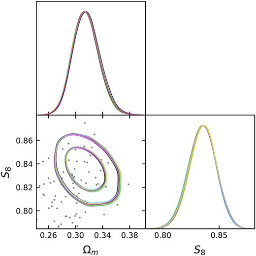
(S8, Ωm) constraints for a given noisy realization of the DES-Y3 3×2pt data vector analysed using 100 lognormal covariance matrices, each computed from a different cosmology drawn from a simulated DES-Y3 3×2pt posterior. The 100 contours are superimposed in the plot, showing very small change in constraints. The points indicate the cosmologies at which the covariances were evaluated.
These results all confirm that we can safely neglect the impact of the choice of covariance cosmology in DES-Y3 3×2pt analysis. One caveat of this conclusion is that we have indeed only varied cosmological parameters (including galaxy bias parameters) but not nuisance parameters (multiplicative shear bias, photometric redshift uncertainties) or parameters that describe intrinsic alignment. However, the DES-Y3 shear and photo-z calibration yield tight Gaussian priors on the corresponding nuisance parameters. Also, intrinsic alignment is relevant only on small angular scales where the covariance matrix is dominated by sampling noise contributions. Hence, we do not expect the results of this section to change significantly had all parameters been varied.
6.9 Random point shot noise
We stress that the Landy–Szalay estimator was devised at a time of very limited computational resources, where it was prohibitively costly to measure galaxy pair in a large number of random points. Hence, it was vital to minimize random point shot noise. Nowadays, footprint geometries of photometric surveys are typically characterized by high-resolution healpix maps. The most straightforward way to calculate galaxy clustering correlation function is to simply assign a value of galaxy density contrast to each of these pixels and then measure the scalar autocorrelation function of the unmasked pixels. This way, one is avoiding random point shot noise completely.
Nevertheless, it is still very common to measure w(θ) by means of equation (79). So we also tested what impact a finite number of random points would have on our analysis. To do so, we extended expressions of Cabré & Gaztañaga (2009; see their appendix A) to the case where the same random points are used to estimate w(θ) in each of our redshift bins and also to subtract shear around random points from our galaxy–galaxy lensing correlation functions. Note that this causes a noise contribution to the two-point function measurements that is correlated among different redshift bins. We assumed a random point density of 1.36 arcmin−2, which is more than 20 times larger than the density of our most dense lens galaxy sample. From Table 1, it can be seen that not accounting for the random point shot noise in the covariance leads to an increase in average χ2 of |${\lesssim} 1{{\ \rm per\ cent}}$| and to an underestimation of parameter uncertainties by |${\approx} 0.5{{\ \rm per\ cent}}$|. Hence, this effect can be ignored for our analysis.
6.10 Effective densities and effective shape noise
We are closing this section by spelling out an aspect of covariance modelling that may seem straightforward but which has repeatedly came up in covariance discussions.
If the tracer galaxies used to estimate two-point correlation functions are weighted according to some weighting scheme, then this may change the effective number densities and the effective shape noise that should be used when evaluating the covariance expressions in Section 4. In the following, we will derive how this can be done for each of the two-point functions in the DESY3 3×2pt data vector.
6.10.1 Galaxy clustering
We start with the galaxy clustering correlation function w(θ). We assume a weighting scheme that is aimed at correcting for non-cosmological density fluctuations resulting from spatially varying observing conditions (as e.g. in Elvin-Poole et al. 2018). This means that the weights assigned to each galaxy in fact sample a weight map that spans the entire footprint.
The first factor on the right-hand side of equation (85) is what the shot-noise variance of |$\hat{w}$| should be in the absence of a weighting scheme. The second term is a two-point function of the weight map itself. If the weight map has a white-noise power spectrum, then this factor will be close to 1 in any angular bin that does not include angular distances of 0. This means that at large enough scales the last line of equation (85) looks like the covariance for plain Poissonian shot noise without any notion of an effective number density. This may be surprising, but it stems from the fact that the weighting scheme we assumed does not simply multiply the galaxy density contrast field. Instead, it reverses an already existing depletion of galaxy density from non-cosmological density fluctuations.
6.10.2 Galaxy–galaxy lensing
One subtlety here is that the above derivation requires |$\langle w_j^s \rangle = 1$|. The above expressions must be modified as this is not the case or when taking into account responses Rj of a shape catalogue generated with metacalibration (Sheldon & Huff 2017). We detail what to do in the latter case in Appendix G.
6.10.3 cosmic shear
6.10.4 Testing validity of effective shape noise
To test the validity of our expression for effective shape noise in equation (90), we run a sub-sample covariance estimator on our data (see e.g. Friedrich et al. 2016). In particular, we divide all of our source and lens galaxy samples into 200 randomly chosen sub-samples and measure the galaxy–galaxy lensing correlation function of each source–lens bin combination. As a result, we obtain 200 measurements of |$\hat{\gamma }_t$| in each source–lens bin combination. Since we employ completely random sub-sampling, i.e. without any regard for e.g. a division of our footprint into sub-regions, the sample covariance of these 200 measurements will almost exclusively be dominated by shape noise and shot noise. This is even more so, because the lens and source densities of the sub-samples are very low.
In Fig. 12, we show the ratio of the variances of the 200 galaxy–galaxy lensing measurements |$\hat{\gamma }_t$| in the different lens–source bin combinations to equation (89). Assuming that the sub-sample covariances follow a Wishart distribution, we find that these ratios are perfectly consistent with 1. This indicates that equation (90) indeed yields an accurate effective shape-noise dispersion, and that one should indeed use the plain density of lens galaxies (as opposed to any notion of effective density) when evaluating covariance expressions.
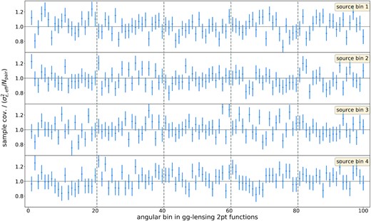
Ratio between the sample variance of |$\hat{\gamma }_t$| measured in 200 randomly selected sub-samples of the DESY3 lens and sources catalogues and equation (89) for the shape-noise contribution to the covariance (again using equation 90 to calculate the effective shape-noise dispersion σϵ,eff). Each row displays the variances measured for a different source redshift bin and vertical dashed lines separate points belonging to different lens redshift bins (1–5 from left to right). Assuming that the covariance estimates have a Wishart distribution, we calculate the covariance matrix of these ratios (cf. Taylor et al. 2013) and find that they are consistent with 1 (both for the cosmic shear and galaxy–galaxy lensing variances).
7 A SIMPLE χ2 TEST
In this short section, we present a simple χ2 test that does not rely on the linearized framework. However, it has the disadvantage of not addressing the impact on the estimation of parameters. Here, we generate a large number of ‘contaminated’ data vectors (we use 1000) by a Gaussian sampling of a given covariance matrix that includes different effects and to compute a χ2 distribution from these data vectors using a fiducial covariance matrix. The resulting shifts in the mean value of χ2 and their standard deviations give another benchmark for the importance of the different effects considered here. We show the results of this test in Fig. 13. Note that the relative increases in χ2 follow closely what we obtained within the linearized likelihood framework in Fig. 1. This indicates that the dominant way in which covariance errors cause χ2 offsets is not through the altered scatter of maximum posterior parameter locations but simply through using an erroneous inverse covariance when computing χ2. That also justifies our usage of the linearized likelihood framework since any impact of non-linear parameter dependences on parameter fitting can be expected to be even less relevant than linear fitting in the first place.
χ2 tests taking into account different effects. Colours follow the scheme of Fig. 1.
8 DISCUSSIONS AND CONCLUSIONS
In this paper, we have presented the fiducial covariance model of the DES-Y3 joint analysis of cosmic shear, galaxy–galaxy lensing, and galaxy clustering correlation functions (the 3×2pt analysis). We then investigated how the assumptions and approximations of that model (including the assumption of Gaussian statistical uncertainties) impact the distribution of maximum posterior χ2 and maximum posterior estimates of cosmological parameters.
The fiducial covariance matrix of the DES-Y3 3×2pt analysis uses the formalism of Krause & Eifler (2017) to model supersample covariance as well as the trispectrum contribution to the covariance. The model for the Gaussian covariance part (i.e. the contributions from the disconnected four-point function) correctly takes into account sky curvature and includes analytical averaging over the finite angular bins in which the two-point functions are measured. Furthermore, the galaxy clustering power spectra that enter our calculation of the Gaussian covariance part are computed using the non-Limber formalism of Fang et al. (2020b) and also include modelling of RSDs. The finite survey area of DES-Y3 is incorporated in the covariance model via the fsky approximation (except in the pure shape-noise and shot-noise terms where we follow Troxel et al. 2018b).
In order to perform our validation tests for the DES-Y3 covariance matrix, we developed a plethora of new modelling ansatzes and testing strategies that are applicable in general. These new techniques are as follows:
We have motivated and devised a way of drawing realizations of the 3×2pt data vector from a non-Gaussian distribution in order to test the accuracy of our Gaussian likelihood assumption.
We have derived analytical expressions for angular bin averaging of all four types of two-point correlation functions included in the 3×2pt vector (ξ+, ξ−, γt, and w). These expressions correctly account for sky curvature. To the best of our knowledge, an analytical treatment of bin averaging for cosmic shear two-point function has not been presented before (though we have shared our results with Fang et al. 2020a, who have used them for the fiducial covariance computations).
We have extended the lognormal analytical model for the covariance of cosmic shear two-point function of Hilbert et al. (2011) to the other two-point functions present in the 3×2pt data vector.
Within a linearized likelihood formalism, we have analytically derived how covariance model inaccuracies influence the distribution of maximum-posterior χ2 and of maximum-posterior parameter estimates. The results we presented also allow for the possibility of including the Gaussian priors on certain model parameters and can be used to analytically estimate the impact of covariance errors on cosmological likelihood analyses.
By fitting an effective number density to the high-ℓ plateau of galaxy clustering Cℓ measurements, we have estimated how much the assumption of Poissonian shot noise influences our likelihood analysis. This is similar in spirit to the RASCALC technique presented by Philcox et al. (2020), and we agree with those authors that non-Poissonian shot noise can be viewed as an effective description of how short-scale non-linearities in galaxy clustering influence the covariance.
We calculated covariance matrices for 100 different sets of cosmological and nuisance parameters randomly drawn from a simulated likelihood chain. This allowed us to investigate whether calculating our covariance model at a reasonable, but wrong point in parameter space significantly impacts our analysis. This was done both within our linearized likelihood framework and by using importance sampling to quickly evaluate the 100 non-linear likelihoods.
We have derived how the two-point correlation function of weight maps influences the covariance of galaxy clustering two-point function measurements. In that context, we have also found that traditional ways of deriving an effective number density for a given set of galaxy weights are erroneous when those weights are aimed at undoing a suspected depletion of galaxy density (e.g. due to variations in observing conditions).
We have derived an expression for the effective dispersion of intrinsic source shapes for the situation when source galaxy weights are correlated with galaxy ellipticity. We have also shown how metacalibration responses (Sheldon & Huff 2017) enter that expression for effective shape noise.
We have described a clean sub-sample covariance estimation scheme that directly measures the sampling noise contributions to the covariance from a given data set. We then used the resulting covariance estimates to test the validity of our assumed effective shape noise values.
We have employed the hybrid covariance estimation technique PME (Friedrich & Eifler 2018) to efficiently evaluate the importance of individual contributions to the covariance from only a limited set of simulated data (in our case: 200 realizations of the 3×2pt data vector including shape noise and 100 realizations without shape noise).
We have devised a treatment of survey geometry in covariance modelling that improves upon existing approximations (of e.g. Efstathiou 2004) and we have demonstrated how to carry those approximations from harmonic space to real space.
Using these results, we perform several tests for the fiducial DES-Y3 3×2pt covariance matrix and likelihood model, with the following conclusions:
The assumption of Gaussian statistical uncertainties is sufficiently accurate (cf. Section 6.1). Hence, knowledge of the covariance of the 3×2pt data vector is sufficient to model our statistical uncertainties. The main assumption made to arrive at this conclusion is that non-Gaussian error bars are primarily a large-scale problem and that at small scales the number of modes present within the DES-Y3 survey volume converges to a Gaussian distribution via the central limit theorem.
The non-Gaussian part of the covariance has a negligible impact on both maximum posterior χ2 and parameter constraints (cf. Section 6.2). This statement is not a general one but only holds for the specific DES-Y3 3×2pt analysis set-up. The main assumption made to arrive at that conclusion is that the CosmoLike model (Krause, Eifler & Blazek 2016) or the lognormal model (Hilbert et al. 2011) for the non-Gaussian covariance does not vastly underestimate the true covariance. Given the results of Sato et al. (2009) and Hilbert et al. (2011), we find that this a safe assumption.
Of all covariance modelling assumptions investigated in this paper, the fsky approximation (made in the mixed term and cosmic variance term of our covariance model) has the largest effect on maximum posterior χ2. On average, it increases χ2 between measurement and maximum posterior model by about |$3.7{{\ \rm per\ cent}}$| (Δχ2 ≈ 18.9) for the 3×2pt data vectors and by about |$5.7{{\ \rm per\ cent}}$| (Δχ2 ≈ 16.0) for the 2×2pt data vector (cf. Table 1).
However, neither fsky approximation nor any other covariance modelling detail tested in this paper (cf. Table 1; with the exception of finite bin width; see the next point) has any significant impact on the location and width of constraints on the parameters Ωm, σ8, and w.
The only exception to this statement is finite angular bin width that – if not taken into account in the mixed term and cosmic variance term of the covariance model – significantly increases the scatter of maximum posterior parameters (without increasing the inferred constraints accordingly). However, finite bin width has been taken into account in the past in an approximate manner – see e.g. Krause et al. (2017).
The fact that we do not know the true cosmological parameters of the Universe forces us to evaluate our covariance model at a wrong set of parameters. Even when iteratively adjusting those parameters to the maximum posterior parameters of the analysis, the parameters of the covariance model will scatter around the ‘true’ cosmological/nuisance parameters. We consider this an irreducible covariance error and find that it increases the maximum posterior scatter of Ωm and σ8 by about |$3{{\ \rm per\ cent}}$| and that of the dark energy equation-of-state parameter w by about |$5{{\ \rm per\ cent}}$| (cf. Section 6.8 and Table 1). At the same time, we find this effect to have a negligible impact on maximum posterior χ2.
In summary, we have shown that our fiducial covariance and likelihood model underestimates the scatter of maximum posterior parameters by about 3–|$5{{\ \rm per\ cent}}$|, which is mostly caused by uncertainty in the set of cosmological and nuisance parameters at which we evaluate that model. On average, the χ2 between maximum posterior model and measurement of the 3×2pt data vector will be |${\sim} 4{{\ \rm per\ cent}}$| higher than expected with perfect knowledge of the covariance matrix. This is mainly caused by our use of the fsky approximation. We have devised an improved treatment of the full survey geometry (cf. Section 6.6) but for the reason mentioned above this was only used to test the impact of the fsky approximation on parameter constraints.
Given the small impact that we estimated from the unaccounted effects in the covariance modelling, we conclude that the fiducial covariance model is adequate to be used in the 3×2pt DES-Y3 analysis. While our validation of this covariance model has been carried out with a preliminary set of scale cuts and redshift distributions, we do not expect qualitative changes for the final DES-Y3 analysis set-up.
While the DESY3 specific outcomes of our study cannot straightforwardly be transferred to other surveys and analyses, our methodological innovations will be useful tools in the covariance and likelihood validation of future experiments.
ACKNOWLEDGEMENTS
OF gratefully acknowledges support by the Kavli Foundation and the International Newton Trust through a Newton-Kavli-Junior Fellowship and by Churchill College Cambridge through a postdoctoral By-Fellowship. The authors thank Henrique Xavier for very helpful discussions about mock simulations and the flask code. This research was partially supported by the Laboratório Interinstitucional de e-Astronomia (LIneA), the Brazilian Funding agency CNPq, the INCT of the e-Universe, and the Sao Paulo State Research Agency (FAPESP). The authors acknowledge the use of computational resources from LIneA, the Center for Scientific Computing (NCC/GridUNESP) of the Sao Paulo State University (UNESP), and from the National Laboratory for Scientific Computing (LNCC/MCTI, Brazil), where the SDumont supercomputer (sdumont.lncc.br) was used.
This paper has gone through internal review by the DES collaboration. Funding for the DES Projects has been provided by the U.S. Department of Energy, the U.S. National Science Foundation, the Ministry of Science and Education of Spain, the Science and Technology Facilities Council of the United Kingdom, the Higher Education Funding Council for England, the National Center for Supercomputing Applications at the University of Illinois at Urbana–Champaign, the Kavli Institute of Cosmological Physics at the University of Chicago, the Center for Cosmology and Astro-Particle Physics at the Ohio State University, the Mitchell Institute for Fundamental Physics and Astronomy at Texas A&M University, Financiadora de Estudos e Projetos, Fundação Carlos Chagas Filho de Amparo à Pesquisa do Estado do Rio de Janeiro, Conselho Nacional de Desenvolvimento Científico e Tecnológico and the Ministério da Ciência, Tecnologia e Inovação, the Deutsche Forschungsgemeinschaft, and the Collaborating Institutions in the DES.
The Collaborating Institutions are Argonne National Laboratory, the University of California at Santa Cruz, the University of Cambridge, Centro de Investigaciones Energéticas, Medioambientales y Tecnológicas-Madrid, the University of Chicago, University College London, the DES-Brazil Consortium, the University of Edinburgh, the Eidgenössische Technische Hochschule (ETH) Zürich, Fermi National Accelerator Laboratory, the University of Illinois at Urbana–Champaign, the Institut de Ciències de l’Espai (IEEC/CSIC), the Institut de Física d’Altes Energies, Lawrence Berkeley National Laboratory, the Ludwig-Maximilians Universität München and the associated Excellence Cluster Universe, the University of Michigan, the National Optical Astronomy Observatory, the University of Nottingham, The Ohio State University, the University of Pennsylvania, the University of Portsmouth, SLAC National Accelerator Laboratory, Stanford University, the University of Sussex, Texas A&M University, and the OzDES Membership Consortium.
Based in part on observations at Cerro Tololo Inter-American Observatory at NSF’s NOIRLab (NOIRLab Prop. ID 2012B-0001; PI: J. Frieman), which is managed by the Association of Universities for Research in Astronomy (AURA) under a cooperative agreement with the National Science Foundation.
The DES data management system is supported by the National Science Foundation under grant numbers AST-1138766 and AST-1536171. The DES participants from Spanish institutions are partially supported by MINECO under grants AYA2015-71825, ESP2015-66861, FPA2015-68048, SEV-2016-0588, SEV-2016-0597, and MDM-2015-0509, some of which include ERDF funds from the European Union. IFAE is partially funded by the CERCA program of the Generalitat de Catalunya. Research leading to these results has received funding from the European Research Council under the European Union’s Seventh Framework Program (FP7/2007-2013) including ERC grant agreements 240672, 291329, and 306478. We acknowledge support from the Brazilian Instituto Nacional de Ciência e Tecnologia (INCT) e-Universe (CNPq grant 465376/2014-2).
This manuscript has been authored by Fermi Research Alliance, LLC under Contract No. DE-AC02-07CH11359 with the U.S. Department of Energy, Office of Science, Office of High Energy Physics.
This work made use of the software packages getdist (Lewis 2019), chainconsumer (Hinton 2016), matplotlib (Hunter 2007), and numpy (Harris et al. 2020).
We would like to thank the anonymous journal referee for their helpful comments.
DATA AVAILABILITY
The DES-Y3 3×2pt covariance matrix and likelihoods will be made public upon publication of our final data analysis. c++ and python tools to configure flask as described in Section 4.3 are available at https://github.com/OliverFHD/CosMomentum. Tools to compute Gaussian and halomodel covariance are available at https://github.com/CosmoLike/CosmoCov.
Footnotes
hsc.mtk.nao.ac.jp/ssp
kids.strw.leidenuniv.nl
nasa.gov/content/goddard/nancy-grace-roman-space-telescope
In order to deal with the prior volume effect, Joachimi et al. (2020) proposed to report parameter constraints through what they call projected joint highest posterior density. This topic will be addressed in a separate DES paper (Raveri et al., in preparation).
Alternatively, one could investigate the distribution of p-values (or probability to exceed; cf. Hall & Taylor 2019) as opposed to the distribution of χ2.
camb.info
We have shared our results with Fang et al. (2020a), who have used them for their covariance calculations.
from |$\smash{\sum _\ell \frac{2\ell + 1}{2} P_\ell (x) P_\ell (y) = \delta _D(x -y)}$| - see N. Bronstein & A. Semendjajew (1979) for this and other properties of Legendre polynomials.
Note that a factor of 1/isin (θ) is missing in the second line of this equation.
A map of the mask will come with a finally resolution, in which case the fractional values 0 < W < 1 of the mask will describe the completeness of observations within the map resolution.
REFERENCES
APPENDIX A: CURVED SKY FORMALISM
APPENDIX B: AVERAGING CORRELATION FUNCTIONS OVER FINITE BINS
APPENDIX C: MASKING IN REAL SPACE COVARIANCES
DES observations do not cover the entire sky, but are located within a survey mask, described by a function |$W(\mathbf {\hat{n}})$| that is =1 if we have observed the sky at location |$\mathbf {\hat{n}}$| and zero otherwise.18 In this appendix, we derive how this masking changes the covariance of any measured two-point statistics.
To implement this correction, we draw circles within the DES-Y3 survey footprint with radii ranging from 5 to 20 arcmin and measure the masking fraction in these circles. We find that this fraction is |${\approx} 90{{\ \rm per\ cent}}$| across the considered scales. Multiplying the mixed terms in the covariance by that fraction and the cosmic variance terms by the square of that fraction (and using equation C15), we indeed find significant improvement of the maximum posterior χ2 obtained for the flask simulations (cf. lower panel of Fig. 8 as well as Fig. 1).
APPENDIX D: MOTIVATION FOR OUR RE-SCALING ANSATZ FOR MASKING EFFECTS
In Fig. D1, we show the ratio of Npair to |$N_{\mathrm{pair,}f_{\mathrm{sky}}}$| (green dashed lines) and compare it to the ratios of different covariance terms when computed with either the fsky approximation or the approximation of Efstathiou (2004) (cosmic variance term: blue dotted lines; mixed term: solid orange lines). The upper panel of the figure computes these ratios for the galaxy clustering two-point function w(θ) in the first lens bin of our fiducial configuration while the lower panel considers the cosmic shear correlation function ξ+(θ) for our first source bins (other redshift bins and two-point functions behave similarly). For w(θ), these different ratios indeed closely agree with each other. The agreement between the ratio of pair counts and the ratio of the different approximations for the mixed terms is especially striking. It is most likely caused by the fact that for the mixed covariance terms one of the two replacements in equations (D3) and (D4) is actually exact. Even for ξ+(θ), the ratio of the different approximations for the mixed term is well described by the ratio of pair counts on most scales. For the cosmic variance of ξ+(θ), one can on the other hand observe a strong deviation. This does not necessarily signify a breakdown of our arguments but may be caused by the fact that cosmic shear is a spin-2 field. The calculations of Efstathiou (2004) do in fact only hold for scalar fields and our extension of their formulae to shear correlation functions is only approximate (see e.g. Challinor & Chon 2005, for more general calculations). Since we have identified the mixed terms to carry the strongest impact of masking on the total covariance, we do not address this any further. Instead, we consider the agreement between pair count ratios and mixed term ratios observed in Fig. D1 as sufficient justification for the re-scaling ansatz of the different covariance terms presented in Section 6.6.
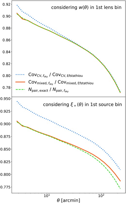
Ratio of exact galaxy pair counts Npair to pair counts computed using equation (D7) (green dashed lines) compared to the ratios of different covariance terms when computed with either the fsky approximation or the approximation of Efstathiou (2004) (cosmic variance term: blue dotted lines; mixed term: solid orange lines).
APPENDIX E: PME TO INVESTIGATE THE IMPACT OF MASKING ON INDIVIDUAL COVARIANCE TERMS
For each flask measurement of the 2×2pt data vector, we estimate the first-order PME from the remaining 196 flask data vectors (respectively from the ∼100 shape-noise free data vectors). The average resulting χ2 values between each data vector and the mean of all data vectors are displayed in Fig. 9 and compared to the χ2 values obtained when applying the analytical masking corrections presented in Section 6.6 to either the shape-noise free covariance terms or the full covariance. The average χ2 when using the analytical, best-guess covariance matrix is ≈318.8 for a total of 302 data points in the 2×2pt data vector. This corresponds to a bias in χ2 of about |$5.5{{\ \rm per\ cent}}$|. The PME estimate of the inverse covariance manages to push this down to ≈307.9 (≈304.8 with our analytic ansatz), hence decreasing the bias in χ2 to about |$1.9{{\ \rm per\ cent}}$| (|$\lt 1{{\ \rm per\ cent}}$| for the analytic ansatz). If the PME correction term is computed with the shape-noise free flask covariance, then the bias only slightly reduces to 〈χ2〉 ≈ 314.3 (≈316.6 with our analytic ansatz). Hence, the shape-noise-dependent mixed terms in the covariance indeed seem to be the main cause of our remaining χ2 offset. This was also found by Joachimi et al. (2020) for the latest analysis of the KiDS. These mixed terms do not depend on the connected four-point function of the density field (cf. Section 3) and the only approximation we make in their calculation is the treatment of our survey footprint through the fsky approximation. Hence, we follow Joachimi et al. (2020) in our conclusion that this approximation is the main driver of the residual errors in our covariance model.
APPENDIX F: IMPACT OF EXTREME COSMOLOGIES ON PARAMETER CONSTRAINTS
To demonstrate that the importance sampling technique employed in Section 6.8 indeed manages to capture even strong changes in the likelihood, we repeat the tests presented there with covariance matrices that drastically differ from our fiducial covariance model. In particular, we shift the value of σ8 for which the covariance model is evaluated by ±2σ of the marginalized σ8 constraints expected from DES-Y3. Note that it is a radical change because it ignores parameter degeneracies; i.e. such a shift of σ8 without changes in other parameters would be detected at high significance. Fig. F1 shows the likelihood contours in the S8–Ωm plane obtained both from our fiducial covariance and from importance sampling with the altered covariance matrices. One can now clearly see a change in contour width. However, as we have shown in Section 6.8, this effect is far less significant for realistic parameter uncertainties in the covariance model.
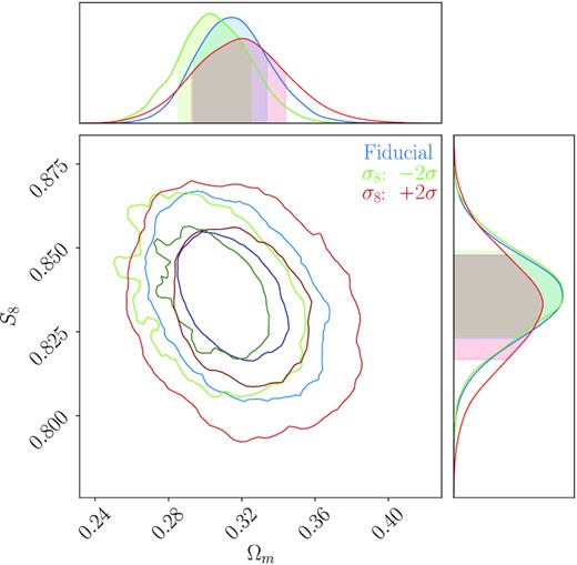
(S8, Ωm) constraints for a given noisy realization of the DES-Y3 3×2pt data vector analysed using: a fiducial covariance matrix (blue); a covariance matrix evaluated at |$\sigma _8 = \sigma _8^\text{fiducial} - 2\sigma _{\sigma _8}$| (green); and a covariance matrix evaluated at |$\sigma _8 = \sigma _8^\text{fiducial} + 2\sigma _{\sigma _8}$| (red). The green and red posteriors were obtained by importance sampling the fiducial samples.
