Chemical abundances in Seyfert galaxies – VIII. Argon abundance estimates Free

ABSTRACT

1 INTRODUCTION

Active galactic nuclei (AGNs) present strong metal emission lines in their optical spectra, which when combined with hydrogen recombination lines, make it possible to estimate the abundance of heavy elements and the metallicity in the gas phase of these objects. AGNs play an essential role in chemical abundance studies of nearby objects and of the early stages of galaxy formation due to the aforementioned feature and to their high luminosity.

Among the heavy elements, oxygen presents strong emission lines (i.e. [O ii]λ3726, λ3729; [O iii]λ5007) emitted by its most abundant ions (⁠|$\rm O^{+}$|⁠, |$\rm O^{2+}$|⁠) in the optical spectrum of gaseous nebulae (H ii regions, Planetary Nebulae) and AGNs (e.g. Koski 1978; van Zee et al. 1998; Kennicutt, Bresolin & Garnett 2003; Maciel, Quireza & Costa 2007; Dopita et al. 2015; Flury & Moran 2020; Dors et al. 2020a). Therefore, the total metallicity (Z) of the gas phase from emission lines emitter objects is commonly traced by the oxygen abundance relative to hydrogen (O/H, e.g. McGaugh 1991; Yates, Kauffmann & Guo 2012; Kewley, Nicholls & Sutherland 2019). Other elements such as the noble gases (e.g. Ne, Ar) present emission lines in the optical spectrum emitted by only few of their ions (e.g. |$\rm Ne^{2+}, Ar^{2+}$|⁠), which make it necessary to apply ionization correction factors (ICFs) proposed by Peimbert & Costero (1969) (see Stasińska 2002; Dors et al. 2013, 2016; Delgado-Inglada, Morisset & Stasińska 2014) in order to account for the unobserved ions in the estimation of the total abundance. The use of ICFs can introduce uncertainties in order of 20 per cent (e.g. Henry, Kwitter & Howard 1996; Alexander & Balick 1997; Croxall et al. 2016) in the resulting total abundance (for a detailed discussion on ICF uncertainties see Delgado-Inglada et al. 2014). Despite this drawback, noble gases can be used to derive the metallicity with some advantages over oxygen, as they are also useful elements for determining constraints in stellar nucleosynthesis studies. Noble gas atoms cannot combine in molecules formation and they can not be trapped in dust grains due to their quantum configuration, unlike the oxygen that is depleted on to dust in order of 0.1 dex (e.g. Izotov et al. 2006; Pilyugin, Thuan & Vílchez 2007).

The T_e-method, which is based on direct estimation of the electron temperature, is widely used in the literature as the most reliable approach for determining the chemical abundance of heavy metals in gaseous nebulae (for a review see Peimbert, Peimbert & Delgado-Inglada 2017; Pérez-Montero 2017). The T_e-method has been bolstered by the consonance between O/H abundance estimates in H ii regions in the solar vicinity and those obtained from observations of the weak interstellar O iλ1356 line towards stars (see Pilyugin 2003 and references therein). Moreover, in the Milky Way and in nearby galaxies, good agreement between O/H abundance estimates in H ii regions and in B-type stars has recently been derived (e.g. Toribio San Cipriano et al. 2017). In this regard, abundance determinations of heavy metals (O, N, S, Ar, etc.) based on the T_e-method have been carried out in thousands of star-forming regions (SFs; i.e. H ii regions, H ii galaxies) at the local universe and for certain objects at high redshifts over decades (see Dors et al. 2020a and reference therein).

Unfortunately, the situation is opposite for AGNs, where, except from oxygen, the majority of the abundances for other elements are not available in the literature. In fact, the most complete metal abundance determinations based on T_e-method was carried out by Osterbrock & Miller (1975) for Cygnus A (z = 0.05607), who derived the O, N, Ne, S, and Fe abundances in relation to hydrogen. After this pioneering work some few studies have applied the T_e-method to abundance estimations in AGNs, however, in most cases, only oxygen abundance determinations have been derived (e.g. Alloin et al. 1992; Izotov & Thuan 2008; Revalski et al. 2018a,b, 2021; Dors et al. 2015, 2020a,b). Recently, Flury & Moran (2020), adopting a methodology based on a reverse engineering of the T_e-method, derived the first (N/O)-(O/H) relation for AGNs. Although studies relied on photoionization models have been applied to derive metal abundance in AGNs (e.g. Stasińska 1984; Ferland & Osterbrock 1986; Storchi-Bergmann et al. 1998; Groves, Heckman & Kauffmann 2006; Feltre, Charlot & Gutkin 2016; Castro et al. 2017; Pérez-Montero et al. 2019; Thomas et al. 2019; Carvalho et al. 2020; Dors et al. 2021; Pérez-Díaz et al. 2021), most of them have produced only estimations for O/H or metallicity. Since the electron temperatures throughout the emission nebula are computed by thermal balancing (see the seminal paper by Williams 1967), the abundances of the most important elements are used as input parameters in photoionization models. All the lines, even if not observed, contribute to the gas cooling rate. In most of the papers which describe the results obtained by using photoionization models, the element relative abundances to H, which were not found to be particularly different from the solar ones, are unfortunately not published in the literature.

The use of photoionization model to derive abundance of different elements other than the oxygen (e.g. N, S, Ar) is (relatively) difficult, hence, it is necessary to find a solution for the electron temperature (or for O/H, the main cooler element) and for the ionization degree of the gas. Afterwards, the lines of the element under study must be adjusted in order to obtain its abundance (see for instance, Pérez-Montero & Díaz 2007; Pérez-Montero et al. 2010; Congiu et al. 2017; Contini 2017; Dors et al. 2017, 2021; Polles et al. 2019). This procedure can produce a degeneracy among nebular parameters, resulting in somewhat uncertain elemental abundances (Morisset et al. 2016; Morisset 2018). In this sense, the use of the T_e-method produces more exact elemental abundance values in comparison with those estimated through photoionization models.

In particular, the argon abundance determination in AGNs is very important in the study of galaxy evolution and stellar nucleosynthesis, since the stellar production and later ejection of this element to the Interstellar Medium (ISM) in the high metallicity regime can be accessed. The stellar nucleosynthesis theory predicts a primary origin for oxygen and argon (also for sulphur and neon) which are predominantly produced on relatively short time-scales by core-collapse supernovae (SNe; massive stars) explosions (e.g. Woosley & Weaver 1995). Thus, assuming a universal initial mass function (IMF),¹ there is expectation for a relatively constant value of the Ar/O abundance ratio with the O/H (or metallicity) variation, as derived by several authors in chemical abundance studies of SFs (e.g. Thuan, Izotov & Lipovetsky 1995; Izotov & Thuan 1999; van Zee & Haynes 2006; van Zee & Haynes 2006; Guseva et al. 2011). However, some authors have found different behaviour of Ar/O with O/H. For example, Izotov et al. (2006), who used a large sample of star-forming galaxies whose observational data were taken from SDSS-DR3 (Abazajian et al. 2005), found that Ar/O abundance ratio decreases by 0.15 dex with the increase of O/H for the range |$\rm 7.1 \: \lesssim \: 12+\log (O/H) \: \lesssim \: 8.5$| (see also Pérez-Montero et al. 2007). On the other hand, recent results from the CHAOS project (Berg et al. 2015) derived by Berg et al. (2020), who applied the T_e-method to 190 individual H ii regions located in nearby galaxies, found Ar/O about constant and similar to the solar value for the range |$\rm 8.3 \: \lesssim \: 12+\log (O/H) \: \lesssim \: 9.0$|⁠, and a high decrease of this abundance ratio for the very low abundance regime. Finally, Kennicutt et al. (2003) hinted that the Ar/O abundance decreases at high metallicity (⁠|$\rm 8.5 \: \lesssim \: 12+\log (O/H) \: \lesssim \: 8.7$|⁠) in the M 101 spiral galaxy.

For the very high metallicity regime (⁠|$\rm 12 +\log (O/H) \: \gtrsim \: 8.8$|⁠), the behaviour of Ar/O with O/H is poorly known as well as its abundance in AGNs. Recently, Dors et al. (2020a) adapted the T_e-method to chemical abundance studies of AGNs, which made it possible to obtain direct O/H estimates up to the very high metallicity regime, i.e. |$\rm 12+log(O/H)\approx 9.3$|⁠, an abundance value which is about 0.3 dex higher than the maximum value obtained for SFs (Pilyugin et al. 2007; Berg et al. 2020). Therefore, abundance studies in AGNs through the T_e-method allow for the calculations of reliable Ar/H abundances in this class of object and further investigating the Ar/O-O/H relation at very high metallicity regime, which is inaccessible in SF abundance studies.

In this context, we used the T_e-method and developed a new methodology based on photoionization model to calculate the abundance of the argon relative to hydrogen in the narrow-line regions (NLRs) of Seyfert 2 galaxies, whose data were taken from the SDSS-DR7 (York et al. 2000). The present study is organized as follows. In Section 2, the observational data and the methodology used to estimate the oxygen and argon abundances are presented. The results and the discussion are presented in Section 3. Finally, the conclusion of the outcome is given in Section 4.

2 METHODOLOGY

To determine the total abundance of the argon and oxygen in relation to hydrogen abundance (Ar/H, O/H), first, we consider optical emission-line intensities of AGNs type Seyfert 2 from Sloan Digital Sky Survey Data Release 7 (SDSS-DR7; York et al. 2000). These observational data were used to calculate the Ar/H and O/H abundances using the T_e-method. We used photoionization models, built with the cloudy code (Ferland et al. 2017), in order to obtain an ICF for the |$\rm Ar^{2+}$| and an estimation of the temperature for the gas region occupied by this ion. In what follows, a description of the observational data and the methodology adopted to obtain the abundances is presented.

2.1 Observational data

We used optical (3000 < λ(Å) < 7200) reddening-corrected emission-line intensities of a sample of Seyfert 2 nuclei obtained from the SDSS-DR7 (York et al. 2000) data made available by MPA/JHU group.² The sample consists of 463 Seyfert 2 nuclei with redshift |$z \: \lesssim \: 0.4$| and stellar masses of the hosting galaxies in the range of |$9.4 \: \lesssim \: \log (M/{\rm M_\odot }) \: \lesssim \: 11.6$| selected by Dors et al. (2020b). From this sample, we considered a sub-sample containing only objects which have the [O ii]λ3726+3729, [O iii]λ4363, [O iii]λ5007, H α, [S ii]λ6716, [S ii]λ6731, and [Ar iii]λ7135 emission lines measured with an error lower than 50  per cent. This criterion reduced the sample to 64 objects out of the 463 selected by Dors et al. (2020b), with redshif in the range of |$0.04 \: \lesssim \: z \: \lesssim \: 0.25$| and range of the stellar masses of the hosting galaxies |$9.9 \: \lesssim \: \log (M/{\rm M_\odot }) \: \lesssim \: 11.2$|⁠.

Figure 1.

Diagnostic diagram log([O iii]λ5007/H β) versus log([N ii]λ6584/H α). Red points represent our sample of Seyfert 2 nuclei (see Section 2.1) whose observational emission-line ratios were taken from the SDSS-DR7 (York et al. 2000) and measured by the MPA/JHU group. The solid black line represents the AGN/star-forming region separation line proposed by Kewley et al. (2001) and given by the equation (1).

Open in new tabDownload slide

The electron density (N_e) of each one of the 64 Seyfert 2 nuclei was calculated from the |$[\rm{ S}\, {\small {II}}]\lambda 6716/\lambda 6731$| line ratio, assuming an electron temperature of 10 000 K, and using the pyneb routine (Luridiana, Morisset & Shaw 2015). In Fig. 2, a histogram with the N_e distribution of our sample is shown. It can be seen that the N_e values for our sample (the maximum value is about 3000 cm⁻³) are lower than the critical density (i.e. |$10^{4-8} \rm \: cm^{-3}$|⁠, see Vaona, Trocar & Hammer 2012) of the emission lines involved in this study therefore effects of collisional de-excitation are negligible in our abundance estimates. In Dors et al. (2020b), a complete description of the selection criteria adopted to obtain the sample as well as a discussion about aperture effects on the abundance determination is presented. Moreover, effects of electron density variation along the AGN radius, X-Ray dominated regions, shock and electron temperature fluctuations in abundance determinations have been discussed by Dors et al. (2020a, 2021) and these are not repeated here.

Figure 2.

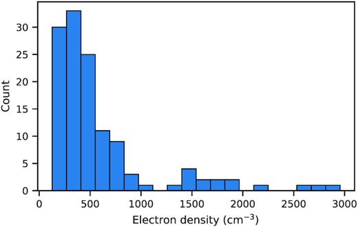
Histogram showing the distribution of electron density values from our sample of 64 objects (see Section 2.1) calculated with PyNeb routine (Luridiana et al. 2015) and considering an electron temperature of 10⁴ K. The y-axis represents the number of object with a given range of electron density value.

Open in new tabDownload slide

2.2 T_e-method

It was possible to estimate the Ar/H and O/H abundances through the T_e-method for the sample of 64 objects. In view of the T_e-method, we followed a similar methodology proposed by Pérez-Montero (2017) and Dors et al. (2020a).

2.2.1 Oxygen abundance

First, for each object, we calculated the temperature of the high ionization gas zone (t₃) and the electron density (N_e) based on the dependence of these nebular parameters on the [O iii](λ4949+λ5007)/λ4363 and [S ii]λ6716/λ6731 line ratios, respectively. We used the function getcrosstemden from the pyneb code (Luridiana et al. 2015), where the value of each parameter was obtained by interacting over the two sensitive line ratios above. The errors in N_e and t₃ were calculated adding a Monte Carlo random-Gauss values to the sample with the function addmontecarloobs in the pyneb code. The symbol t₃ represents the electron temperature in units of 10⁴ K. The mean value derived for t₃ from our sample is ∼1.5 and the uncertainty is ∼0.3. For the electron density, we found a mean value of |$470 \: \rm cm^{-3}$| and an uncertainty of |$\sim 250 \: \rm cm^{-3}$|⁠.

2.2.2 Argon abundance

However, Dors et al. (2020a) showed that, in general, AGNs present a distinct electron temperature structure than H ii regions (see also Armah et al. 2021; Dors et al. 2021; Riffel et al. 2021). Thus, it is worthwhile to ascertain the validity of equations (6) and (7) for AGNs. In view of this, we used the results from the photoionization model grid by Carvalho et al. (2020) and considered predictions for |$T_{\rm e}(\rm{ A}\, {\small {III}})$| and |$T_{\rm e}(\rm{ S}\,\small {III})$|⁠. This grid of photoionization models considered a wide range of AGN nebular parameters whose optical predicted emission lines reproduce those of a large sample of Seyfert 2 nuclei (for a detailed description of these models see Carvalho et al. 2020). The temperature values predicted by the photoionization models and considered here correspond to the mean temperature for |$\rm Ar^{2+}$| and |$\rm S^{2+}$| over the nebular AGN radius times the electron density. In Fig. 3, bottom panel, the photoionization model predictions for |$T_{\rm e}(\rm{ S}\, \small {III})$| versus |$T_{\rm e}(\rm{ Ar}\, \small {III})$| (in units of 10⁴ K) and the approach given by equation (6) are shown. It can be seen that, in contrast to H ii regions, |$T_{\rm e}(\rm{ A}\, \small {III})$| is generally higher than |$T_{\rm e}(\rm{ S}\, \small {III})$|⁠, indicating that equation (6) is not valid for AGN abundance studies. The same can be seen in Fig. 3, top panel, where the AGN model predictions show a large deviation from the temperature relation given by equation (7).

Figure 3.

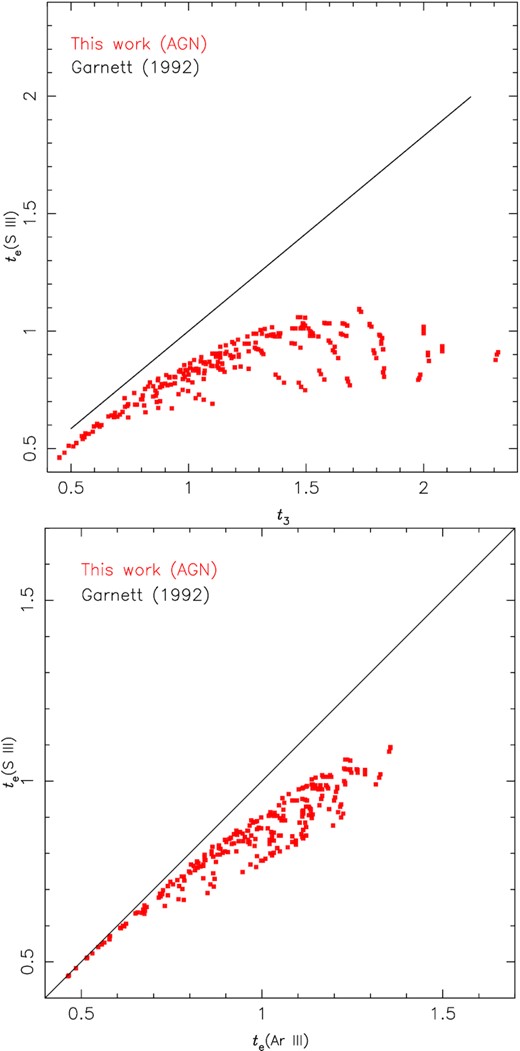
Temperature values for the |$\rm S^{2+}$|⁠, |$\rm Ar^{2+}$|⁠, and |$\rm O^{2+}$| predicted by the photoionization models built by Carvalho et al. (2020) by using the cloudy code (Ferland et al. 2013). The values correspond to the model predicted mean temperature (in units of 10⁴ K) for each ion over the nebular AGN radius times the electron density. Bottom panel: temperature values for the |$\rm S^{2+}$| versus those for |$\rm A^{2+}$|⁠. The black line corresponds to equality between the temperatures (equation 6) proposed by Garnett (1992) for H ii regions. Red points represent photoionization model results. Top panel: same as the bottom panel but for |$\rm S^{2+}$| versus t₃, where t₃ represents the temperature for |$\rm O^{2+}$|⁠. Black line represents equation (7) proposed by Garnett (1992).

Open in new tabDownload slide

Figure 4.

Same as Fig. 3 but for |$T_{\rm e}(\rm{ Ar}\, \small {III})$| versus t₃. Black curve represents a fit to the points represented by equation (8).

Open in new tabDownload slide

Figure 5.

ICF for |$\rm Ar^{2+}$| (as defined in equation 10) as a function of the |$\rm x=[O^{2+}/(O^{+}+O^{2+})]$| abundance ratio. Points represent results from photoionization models built by Carvalho et al. (2020). Model results assuming different metallicities (in relation to the solar value) are represented by different colours, as indicated. The curve represents a fit to all the points given by the equation (11).

Open in new tabDownload slide

Figure 6.

Bi-parametric calibration among the |$\rm ICF(Ar^{2+})$|⁠, |$\rm 12+\log (O/H)$|⁠, and |$\rm x=[O^{2+}/(O^{+}+O^{2+})]$|⁠. Points represent the photoionization model results built by Carvalho et al. (2020) while the surfaces represent the best fit to the points. The blue surface is given by equation (13) and valid it is for |$\rm \mathit{ x} \: \lt \: 0.6$| while the green surface, given by equation (14), is valid for |$\rm \mathit{ x} \: \gt \: 0.6$|⁠.

Open in new tabDownload slide

The expressions above were applied to derive the total abundance of the argon in relation to the hydrogen (Ar/H).

The mean errors for the 12+log(Ar/H) and 12+log(O/H) abundances derived for the objects of our sample are ∼0.25 and ∼0.13 dex, respectively. These errors are in order of those derived for O/H abundance determinations in nearby AGNs by Revalski et al. (2018a,b, 2021), who also applied the T_e-method. However, they are somewhat (∼0.1 dex) higher than those derived for disc H ii regions located in nearby galaxies (e.g. Berg et al. 2020), because the [O iii]λ4363 auroral line is weaker in AGNs than in H ii regions, resulting in a higher uncertainty in its flux, which in turn implies a larger uncertainty in the AGN abundance values.

In Table 1, the SDSS identification of the objects of the sample, electron temperature and electron density values, argon ICF values, ionic and total abundances, redshift, and stellar mass of the hosting galaxies are listed.

3 RESULTS AND DISCUSSION

Figure 7.

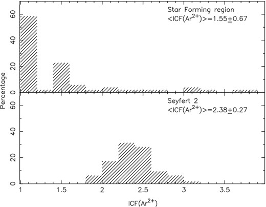
Bottom panel: distribution of the ICF values for the argon from our sample of Seyfert 2 (see Section 2.1) derived by using equations (13) and (14). The averaged value is indicated. Top panel: Same as the bottom panel but for ICFs of SFs (H ii regions and H ii galaxies) derived by Berg et al. (2020, 2015), Croxall et al. (2015, 2016), Bresolin et al. (2009), Hägele et al. (2008), and Lee & Skillman (2004).

Open in new tabDownload slide

Regarding abundance estimates, our results for Seyfert 2 nuclei can be used to verify a possible secondary stellar production of the argon at the very high metallicity regime |$\rm [12+log(O/H) \: \gtrsim \: 8.8]$|⁠, because the maximum value derived in most part of SFs through the T_e-method is in the order of 12+log(O/H)∼8.7 (e.g. Kennicutt et al. 2003; Berg et al. 2020; Yates et al. 2020). In Fig. 8, the total argon abundance [in units of 12+log(Ar/H)] versus the oxygen abundance [in units of 12+log(O/H)] from our sample of Seyfert 2 nuclei is shown. Also in this figure, abundance results based on T_e-method for galaxy nuclei with star formation derived by Izotov et al. (2006) (whose observational data were also taken from SDSS; Abazajian et al. 2005) as well as results for H ii galaxies obtained by Hägele et al. (2008) are shown. In this case, we chose to compare our results only with those from star-forming galaxies (excluding disc H ii regions) because SFs are subject to similar physical processes like those in AGNs. The following are few examples which underscore such similarities.

• SFs and AGNs can present gas outflows (e.g. Hopkins et al. 2012; Hirschmann et al. 2013; Riffel, Storchi-Bergmann & Riffel 2014; Chisholm et al. 2017; Riffel et al. 2021; Riffel 2021; Couto et al. 2021).

• In the case of spiral galaxies the presence of bars might produce a falling of gas into the central regions in both objects (e.g. Athanassoula 1992).

Figure 8.

Total argon abundance [in units of 12+log(Ar/H)] versus the oxygen abundance [in units of 12+log(O/H)]. Red points represent abundance results from our sample of Seyfert 2. Black points represent abundance results from H ii galaxies obtained through T_e-method by Izotov et al. (2006) and Hägele et al. (2008). The solid line represents a fit to the points (equation 16) while the dashed lines represent the uncertainty of ±0.1 dex in H ii region abundance estimations (e.g. Kennicutt et al. 2003).

Open in new tabDownload slide

The heavy elements in AGNs are mainly produced by stellar evolution in the ISM located at few kpc away from the nuclei (e.g. Boer & Schulz 1993; Elmegreen et al. 2002; Díaz et al. 2007; Böker et al. 2008; Dors et al. 2008; Riffel et al. 2009; Hägele et al. 2013; Álvarez-Álvarez et al. 2015; Riffel et al. 2016; Pilyugin et al. 2020; Ma et al. 2021) and then transported to the supermassive black hole. Additional metal enrichment by stars can also be obtained by two ways:

• |$in\, situ$| star formation embedded in the thin AGN accretion disc (e.g. Collin & Zahn 1999; Goodman & Tan 2004; Collin & Zahn 2008; Wang et al. 2011; Mapelli et al. 2012; Davies & Lin 2020; Cantiello, Jermyn & Lin 2021) and by

• capture of stars orbiting the central regions of galaxies (e.g. Syer, Clarke & Rees 1991; Artymowicz, Lin & Wampler 1993).

Both processes can produce different chemical evolution of AGNs in comparison with that of SFs. For instance, the maximum oxygen abundance in the centres of most luminous star-forming galaxies has been found to be 12+log(O/H)∼8.9 (e.g. Pilyugin et al. 2007) while Seyfert 2 nuclei can reach up to ∼9.2 dex (e.g. Dors et al. 2020a; Dors 2021), i.e. there is an additional enrichment in Seyferts in comparison with metal-rich H ii regions. Moreover, recently, Armah et al. (2021) found that Ne/H abundance in a small sample of Seyfert 2s is nearly 2 times higher than those in SFs. Thus, determining metal abundance in AGNs, in this case argon abundance, can produce constraints in studies on star nucleosynthesis in the very high metallicity regime and in different boundary conditions than those in SFs.

Figure 9.

Left-hand panel: distribution of argon abundance [in units of 12+log(Ar/H)] for our sample of Seyfert 2 nuclei. The red line represents the solar argon abundance [|$\rm 12+log(Ar/H)_{\odot }=6.40$|] derived by Grevesse & Sauval (1998). Right panel: same as the left-hand panel but for log(Ar/O). The red line represent the solar argon abundance [|$\rm \log (Ar/O)_{\odot }=-2.29$|] derived by Grevesse & Sauval (1998) and Allende Prieto et al. (2001).

Open in new tabDownload slide

Figure 10.

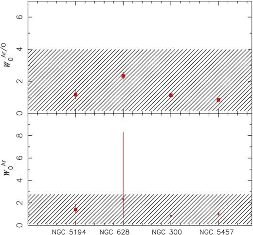
Comparison between argon abundance in relation to the solar value for |$W_{0}^{\rm Ar}=\rm (Ar)/(Ar)_{\odot }$| (bottom panel) and |$W_{0}^{\rm Ar/O}=\rm (Ar/O)/(Ar/O)_{\odot }$| (top panel). Points represent estimates from radial abundance extrapolations to the central parts (galactocentric distance R = 0) from the four spiral galaxies listed in Table 3 and indicated in the x-axis. The hatched areas represent the range of abundance ratio values derived for our sample of Seyfert 2 listed in Table 2.

Open in new tabDownload slide

Figure 11.

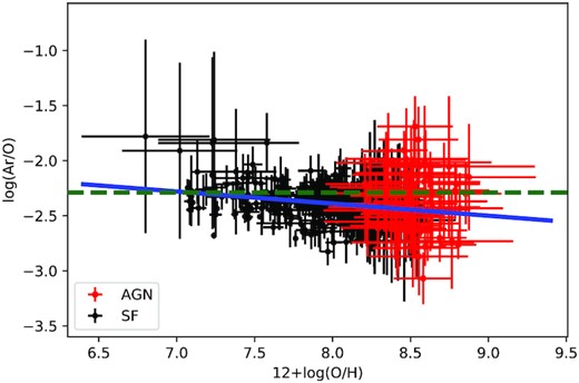
Relation between log(Ar/O) and 12+log(O/H). Red points represent estimations for our sample of Seyfert 2 while black points represent compiled estimations for H ii galaxies derived by Izotov et al. (2006) and Hägele et al. (2008). The blue solid line represents the linear regression to the points given by equation (20). The dashed green line represents the solar value, log(Ar/O)_⊙ = −2.29, derived by Grevesse & Sauval (1998) and Allende Prieto et al. (2001).

Open in new tabDownload slide

4 CONCLUSIONS

For the fist time, quantitative argon abundances, based on T_e-method adapted for AGNs, are derived for the narrow regions of Seyfert 2 nuclei. In view of this, we compiled from Sloan Digital Sky Survey Data Release 7 (SDSS-DR7) optical narrow emission line fluxes for 64 Seyfert 2 galaxies in the local universe (z < 0.25) and calculated the abundance of the argon and oxygen in relation to hydrogen (Ar/H, O/H). The total argon abundance relative to hydrogen (Ar/H) was derived for each object of the sample through the |$\rm Ar^{2+}/H^+$| ionic abundance and by using a theoretical expression for the Ionization Correction Factor (ICF) obtained from photoionization model results built with the cloudy code. These results from the models were also used to derive an appropriate temperature for the |$\rm Ar^{2+}$| [|$T_{\rm e}(\rm{ Ar}\, {\small {III}})$|] which can be derived by its dependence on the temperature for |$\rm O^{2+}$| [|$T_{\rm e}(\rm{ O}\, {\small {III}})$|] calculated by using the observational [O iii](λ4959+λ5007)/λ4363 line ratio. We obtained the following conclusions:

• The equality between the temperatures |$T_{\rm e}(\rm{ S}\, \small {III})$|=|$T_{\rm e}(\rm{ Ar}\, {\small {III}})$|⁠, usually assumed in abundance studies of star-forming regions, is not valid for Seyfert 2 since the nebular gas region occupied by |$\rm Ar^{2+}$| tends to have a lower temperature than the nebular gas region occupied by |$\rm S^{2+}$|⁠.

• A bi-parametric expression for the ICF(⁠|$\rm Ar^{2+}$|⁠) as function of the |$\rm x=[O^{2+}/(O^{+}+O^{2+})]$| abundance ratio and the oxygen abundance [in units of 12+log(O/H)] is proposed to derive the total argon abundance.

• For the range of oxygen abundance |$\rm 8.0 \: \lesssim \: [12+\log (O/H)] \: \lesssim \: 9.0$| or metallicity |$0.20 \: \lesssim \: (Z/\rm \rm Z_{\odot }) \: \lesssim \:2.0$|⁠, we found that our sample of Seyfert 2 present A/H abundances ranging from ∼0.1 to ∼3 times the argon solar value, indicating that most of the objects (⁠|$\sim \!75{{\ \rm per\ cent}})$| have subsolar argon abundance.

• The range of Ar/H and Ar/O abundance values obtained for our sample are in consonance with those estimated from extrapolations to the central parts of radial abundance gradients derived in the disc of four spiral galaxies.

• We found a slight tendency of Ar/O abundance ratio decreases with O/H.

• Finally, the Ar/O abundance values for our sample of Seyfert 2 are in consonance with estimations for H ii galaxies |$[\rm 12+\log (O/H) \: \gtrsim \: 8.0$|], indicating that there is not an over enrichment of argon in AGNs, at least for the metallicity range considered.

ACKNOWLEDGEMENTS

AFM gratefully acknowledges support from Coordenação de Aperfeiçoamento de Pessoal de Nível Superior (CAPES). OLD is grateful to Fundação de Amparo à Pesquisa do Estado de São Paulo (FAPESP) and Conselho Nacional de Desenvolvimento Científico e Tecnológico (CNPq).

DATA AVAILABILITY

The data underlying this article will be shared on reasonable request with the corresponding author.

Footnotes

REFERENCES