


ABSTRACT
Gravitational coupling between protoplanetary discs and planets embedded in them leads to the emergence of spiral density waves, which evolve into shocks as they propagate through the disc. We explore the performance of a semi-analytical framework for describing the non-linear evolution of the global planet-driven density waves, focusing on the low planet mass regime (below the so-called thermal mass). We show that this framework accurately captures the (quasi-)self-similar evolution of the wave properties expressed in terms of properly rescaled variables, provided that certain theoretical inputs are calibrated using numerical simulations (an approximate, first principles calculation of the wave evolution based on the inviscid Burgers equation is in qualitative agreement with simulations but overpredicts wave damping at the quantitative level). We provide fitting formulae for such inputs, in particular, the strength and global shape of the planet-driven shock accounting for non-linear effects. We use this non-linear framework to theoretically compute vortensity production in the disc by the global spiral shock and numerically verify the accuracy of this calculation. Our results can be used for interpreting observations of spiral features in discs, kinematic signatures of embedded planets in CO line emission (‘kinks’), and for understanding the emergence of planet-driven vortices in protoplanetary discs.
1 INTRODUCTION
Gravitational coupling of young planets with the protoplanetary discs in which they form is known to give rise to global spiral density waves. These planet-induced waves may be responsible for the non-axisymmetric structures observed around multiple disc-hosting stars, for example spiral patterns seen in scattered light observations of MWC 758 (Grady et al. 2013; Benisty et al. 2015), SAO 206462 (Muto et al. 2012; Garufi et al. 2013), and other systems.
Density waves launched by planets carry angular momentum and energy, which can be deposited into the disc fluid giving rise to disc evolution (Goodman & Rafikov 2001; Rafikov 2002a, 2016) and gap formation (Lin & Papaloizou 1993; Rafikov 2002b), provided that the wave can be damped either linearly (Takeuchi, Miyama & Lin 1996; Miranda & Rafikov 2020a, b) or non-linearly (Goodman & Rafikov 2001; Rafikov 2002a). Non-linear wave dissipation naturally results from non-linear steepening of the wave profile and its eventual evolution into a shock, even for low wave amplitudes. Irreversible energy dissipation at the shock is the ultimate cause of the non-linear damping of a density wave (Goodman & Rafikov 2001; Rafikov 2016).
The local theory of GR01 has been subsequently extended to global discs in Rafikov (2002a) (hereafter RR02), fully accounting for radial gradients of the protoplanetary disc properties (e.g. cs and gas surface density Σ) and curvature effects. This more general, global framework has in particular allowed Rafikov (2002b) to explore gap opening by migrating planets accounting for the non-locality of non-linear wave damping, which was later verified numerically in Li et al. (2009) and Yu et al. (2010).
The goal of this work is to quantitatively verify the global theoretical framework of RR02 using hydrodynamical simulations. We study various aspects of excitation, propagation, and decay of the density waves driven by subthermal mass (Mp ≲ Mth) planets. Also, following Dong et al. (2011b), we use the global theoretical framework of RR02 to compute vortensity generation by global planet-driven spiral shocks and verify these predictions numerically. There are several key motivations for this study.
First, there has been limited amount of past work trying to verify non-linear propagation of global density waves, mainly documenting the evolution of the wave profile towards the asymptotic N-wave regime (Duffell & MacFadyen 2012) and examining the deviation of the spiral shape from the linear prediction (see Section 5.2; Zhu et al. 2015). Here we aim to provide a systematic study of the wave excitation and evolution, covering a broad range of the relevant parameters – disc aspect ratio hp = Hp/Rp, planet mass Mp, and disc surface density profile Σ(R) – using a variety of diagnostics.
Secondly, theoretical frameworks of GR01 and RR02 reduce the full set of fluid equations to a single inviscid Burgers equation in the limit of a weakly non-linear density wave. So far the accuracy of this approximation (which has been recently employed in Bollati et al. 2021) has not been studied, and we provide its systematic test in this work.
Thirdly, the global theory of RR02 explicitly assumes that a linear effect – excitation of a single-armed spiral wave (Ogilvie & Lubow 2002) by the planetary potential – takes place only close to the planet, and that far from it only non-linear effects regulate wave evolution. However, recent studies (Bae & Zhu 2018; Miranda & Rafikov 2019a) have shown that linear effects (in the form of evolving interference of the individual modes comprising the wave profile) continue driving wave evolution in the disc interior to the planetary orbit even far from the planet, leading to an evolution of a single-armed density wave into multiple arms. This work will examine how this effect modifies the picture of global density wave propagation in discs.
This paper is structured as follows. In Section 2, we describe our physical setup and summarize the key ingredients of the global wave evolution theory of RR02. Upon describing our numerical tools in Section 3, we present results on the non-linear evolution of the global planet-driven density waves for different planet masses in Section 4, as well as the fitting formulae for the resultant shock strength and shape in Section 5. In Section 6 and Appendix C, we develop a framework for computing the vortensity production by the planet-driven spiral shock and verify it numerically. We explore the effect of varying disc parameters on wave evolution in Section 7. Our results are further discussed in Section 8 and summarized in Section 9.
2 PROBLEM SETUP AND THEORETICAL BACKGROUND
In this section, we first describe the physical setup for the problem under consideration (Section 2.1), and then provide relevant theoretical background (Sections 2.2 and 2.3).
2.1 Problem setup
We consider a planet of mass Mp orbiting a central star of mass M⋆ on a circular orbit with a semimajor axis Rp that lies within a 2D gas disc. The 2D approximation is appropriate for thin discs, such that the disc aspect-ratio h = H/R = cs/(ΩR) ≪ 1. Planetary gravity perturbs the motion of disc fluid, giving rise to a density wave that we explore in this work. We adopt polar coordinates (R, ϕ) to describe this problem.
For all our models, we adopt a globally isothermal equation of state (EoS), |$P = c_\mathrm{s}^2 \Sigma$|, where P is the vertically integrated pressure, Σ is the surface density, and cs is the spatially constant speed of sound. We opted to use this barotropic EoS instead of an often used non-barotropic locally isothermal EoS, for which the sound speed follows a prescribed radial profile cs(R), for several reasons.
First, it has recently been shown by Miranda & Rafikov (2019b, 2020a, b), that the use of a locally isothermal EoS leads to a non-conservation of angular momentum flux (AMF) of the density waves freely propagating through the disc even in the absence of explicit dissipation. On the other hand, a barotropic EoS (in particular, the globally isothermal EoS) conserves wave AMF after excitation (see also Lin & Papaloizou 2011; Lin 2015), which greatly simplifies our analysis of the problem (see below). Secondly, the globally isothermal assumption eliminates baroclinic vorticity driving, see Section 8.3. Thirdly, the use of this EoS reduces the number of parameters characterizing the problem at hand.
Our fiducial disc model has an aspect ratio at the planet’s radius, hp = 0.05 and a surface density slope p = 3/2. The latter results in an initial vortensity profile that is almost constant for slightly sub-Keplerian discs, see Section 6.
When presenting our results we adopt units where G = M⋆ = ΩK(Rp) = Σ0(Rp) = 1.
2.2 Linear evolution of planet-driven density waves

A snapshot (at t = 740 planetary orbits) from one of our simulations using fiducial disc parameters and an intermediate-mass planet Mp/Mth = 0.25. (a) An R − ϕ map of the normalized surface density perturbation δΣ/Σ0(R). The locations of the primary and secondary spiral arms are indicated by arrows. The linear prediction (equation 21) is shown by the black dotted line. (b) Radial profile of the azimuthally averaged surface density perturbation δΣ/Σ0(R). (c) Radial profile of the azimuthally averaged vortensity perturbation δζ. (d) Map of the vortensity perturbation δζ. The dashed horizontal lines show the predicted shock locations R = Rp ± lsh. This long-term simulation was run at the resolution NR × Nϕ = 3448 × 7200.
However, it has been realized recently that a single-peak structure does not fully capture the shape of the spiral density wave in the inner disc (Dong et al. 2015; Fung & Dong 2015). Instead, far enough from the planet, the wave is comprised of several narrowly spaced (for low Mp) spiral arms, as indicated in Fig. 1(a). This redistribution of AMF was understood in Bae & Zhu (2018) and Miranda & Rafikov (2019a) as a manifestation of linear evolution of the density waves in differentially rotating discs, following from their weakly dispersive nature. It was shown that the interference of different azimuthal harmonics comprising the perturbation pattern evolves in the inner disc in such a way as to cause the appearance of secondary, tertiary, etc. arms after the wave has travelled far enough from the planet. During this process, the primary spiral arm steadily transfers some of its AMF to the secondary (and higher order) spiral(s), thereby decreasing in amplitude even in the absence of any dissipative effects (the full wave AMF is conserved in the absence of damping in barotropic discs). Arzamasskiy & Rafikov (2018) and Miranda & Rafikov (2019a) have also shown that this phenomenon is not unique to waves driven by a planet, but occurs for any passively propagating density wave. In this work, we will explore how this linear effect impacts non-linear wave evolution.
2.3 Non-linear evolution of global density waves
While the excitation of waves by planets can be described by linear theory, their propagation over large distances is subject to non-linear effects, even for small wave amplitudes. This is the process that ultimately makes waves steepen, form a shock, and dissipate, thus depositing their angular momentum to the disc.
Keeping the most important non-linear terms in their analysis, GR01 have shown that the evolution of weakly non-linear waves can be reduced to a 1D non-linear wave propagation problem described by the inviscid Burgers equation (see below). Their calculation was local as it adopted the shearing-sheet geometry and assumed a uniform background state of the disc. RR02 extended that analysis to the global case by allowing for an inhomogenous, radially structured disc and accounting for the cylindrical geometry, still reducing the problem of wave propagation to the same mathematical form.
We now summarize some key results of GR01 and RR02 regarding propagation of weakly non-linear planet-driven waves.
In the Burgers equation framework (8)–(12) wave evolution is self-similar. In other words, equation (12) does not contain any physical parameters of the problem (Mp, Σ0(R), c0(R), Ωp, etc.), all of which are absorbed into the definitions of variables τ, η, χ, and initial conditions.
For a weakly non-linear wave excited by a planet with Mp ≲ Mth the regions of linear wave excitation (within (1 − 2)Hp from the planet) and its subsequent non-linear propagation are spatially separated.
- As a result of non-linear evolution, the wave inevitably shocks at some radial separation lsh away from the planet. This shocking length is set by the value of τ = τsh at which the characteristics of the Burgers equation (12) first cross. Using the linear wake profile from the excitation region (determined by solving the linearized perturbation equations) as an initial condition for the Burgers equation, GR01 found(15)$$\begin{eqnarray*} \tau _\mathrm{sh} &\simeq \tau _0 + 0.53, \qquad {\rm with} \end{eqnarray*}$$being the point at which the initial conditions are applied. The radial distance from the planet, at which the wave starts to shock (i.e. where τ = τsh) is(16)$$\begin{eqnarray*} \tau _0 &= 1.89 M_\mathrm{p}/M_\mathrm{th} \end{eqnarray*}$$One can see that for Mp ≲ Mth the shocking length lsh indeed lies outside the linear wave excitation region, lsh ≳ Hp.(17)$$\begin{eqnarray*} l_\mathrm{sh} \simeq 0.8 H_\mathrm{p} \left(\frac{\gamma + 1}{12/5} \frac{M_\mathrm{p}}{M_\mathrm{th}} \right)^{-2/5}. \end{eqnarray*}$$
After shocking, the wave profile asymptotically (for τ ≳ τsh) evolves into an N-wave shape (Landau & Lifshitz 1959; Whitham 2011), which is a typical outcome of the wave evolution governed by the Burgers equation. In this regime, the azimuthal width of the wake grows as Δη ∝ τ1/2 while the wave AMF decays as Φ ∝ τ−1/2, which results in |$F_J^\mathrm{WKB} \propto \tau ^{-1/2}$| (GR01).
The behaviour of τ for the two values of surface density slopes p that we consider in this work is shown in Fig. 2. In a uniform disc (p = 0) higher (lower) values of τ are reached in the inner (outer) disc, as compared to the fiducial value p = 1.5, meaning that non-linearity is accelerated (slowed down) in a uniform disc. Also, as can be seen from equation (18), |$\tau \propto h_\mathrm{p}^{-5/2}$|, so that increasing the disc scale height would lead to slower non-linear wave evolution over the same radial distance.

Radial profile of the coordinate τ(R) for the disc profiles considered in this work, as labelled in the legend. The dependence on |$h_\mathrm{p}^{5/2}$| and Mp/Mth is absorbed by rescaling the vertical axis. One can see that for a uniform disc p = 0, non-linearity is accelerated (slowed down) in the inner (outer) disc, as compared to the fiducial value (p = 1.5).
3 NUMERICAL SETUP
We now describe several different numerical tools used in this work.
3.1 Hydrodynamical simulations
In our globally isothermal setup, the energy equation is not solved. Our fiducial setup computes the fluxes at cell-interfaces using second-order accurate (linear) spacial reconstruction and Roe’s approximate Riemann solver. We have performed additional tests using the HLLE solver and found no noticeable differences in our results. The equations are integrated in time using a second-order Runge–Kutta scheme.
The total potential is given by Φ = Φ⋆ + Φp, where the potential due to the central star is Newtonian Φ⋆ = −GM⋆/R and the planet’s potential is Φp. We neglect the indirect potential contribution that arises due to the acceleration of our non-inertial reference frame that is centred on the star. This is mainly to allow a direct comparison to the linear results of Miranda & Rafikov (2019a), who used the same approach.5 We performed tests that include the indirect term and they have shown no noticeable differences in the main results.
We also employ an orbital advection scheme that is based on the FARGO algorithm (Masset 2000). Its implementation in Athena is described by Sorathia et al. (2012). It has now also been implemented in athena+ + and is available in the latest public release (version 21.0). In our models orbital advection is performed at intermediate integration time-steps to keep the scheme second-order accurate in time. In our version, orbital advection is done using the Keplerian background velocity |$\mathbf {u}_\mathrm{K}(R) = \sqrt{GM_\star /R} \hat{e}_\phi$|, which is only a function of R and constant in time. This allows for a larger time-step, leading to a net speed-up of more than one order of magnitude for our typical setup. We find that using this method leads to decreased numerical diffusion as compared to models that do not employ this scheme. We have tested the method carefully, including tests with discs that do not host planets. As an additional check, we also performed several simulations using fargo3d (Benítez-Llambay & Masset 2016) and found good agreement between the results obtained with two different codes, see Appendix B for details.
We vary the parameters of the problem in the following way: the planet mass is Mp/Mth ∈ [0.01, 0.1, 0.25, 0.5, 1], the disc aspect ratio at the planet location is hp ∈ [0.05, 0.07, 0.1], and the background disc surface density slope is p ∈ [0, 1.5].
The simulation domain extends over a radial range 0.2 ≤ R/Rp < 4.0 with logarithmic spacing and uniformly extends over the full azimuthal angle 0 ≤ ϕ ≤ 2π. We employ wave-damping zones (de Val-Borro et al. 2006) close to the radial boundaries in the zones 0.2 ≤ R/Rp ≤ 0.28 and 3.4 ≤ R/Rp ≤ 4 to avoid reflections. Only the radial velocity and density are damped towards their initial values, while the azimuthal velocity remains unchanged.
Probing the evolution of very small perturbations in the inviscid regime requires very high resolution to suppress numerical viscosity, which can lead to linear damping of the wave (e.g. Dong et al. 2011a, b). Regarding this issue, we perform an extensive resolution study to judge the convergence of our results. Resolutions ranged from the lowest NR × Nϕ = 3448 × 7200 up to NR × Nϕ = 27 584 × 57 600. This corresponds to 58 and 464 cells per disc scale-height at the planet radius.
We evolved the lowest resolution cases for about 1000 planetary orbits, while the highest resolution simulations were evolved for 20 orbits, due to their high computational cost.6 However, this is still long enough for the wave to reach a quasi-steady state, as the longest sound crossing time across the domain (for hp = 0.05) is less than 20 planet orbits.
3.2 Linear calculations
To provide a benchmark for athena+ + to meet in the low planet mass limit (Mp ≪ Mth), we use the numerical method of Miranda & Rafikov (2019a) to calculate the global structure of linear perturbations in globally isothermal discs. This calculation, relying on solving the linearized fluid equations in fully global setup, allows us to confirm the precision of the implemented methods in fully non-linear simulations and to demonstrate the transition into weakly non-linear behaviour. For consistency, we employ the same potential |$\Phi _\mathrm{p}^{(4)}$| in these calculations (see also Appendix A).
3.3 Solutions of Burgers equation
Our verification of the weakly non-linear theory described in Section 2.3 relies on solving the inviscid Burgers equation (12) in order to directly obtain wave profiles and to compare their evolution with our simulations results. We numerically solve equation (12) adopting a finite-volume scheme with Engquist-Osher flux-splitting and a second-order Runge–Kutta integrator for stepping in τ. As initial wave profiles, we use data from our non-linear simulations, close to the planet at τ = τ0, where excitation of the wake is expected to be almost complete. This corresponds to R/Rp ≃ 0.936 and R/Rp ≃ 1.068 (in the inner and outer disc) for hp = 0.05.
4 EVOLUTION OF THE PLANET-DRIVEN WAVES AS A FUNCTION OF MP
In this section, we compare different descriptions of the planet-driven density wave evolution for two different planet masses assuming the fiducial disc with a density slope p = 3/2 and aspect ratio at planet location hp = 0.05 (dependence on disc parameters is explored in Section 7). Unless specifically mentioned, e.g. when discussing long-term behaviour, results are shown after 20 planetary orbits, when the initial distribution of Σ in the disc is not yet strongly perturbed.
4.1 The low-mass case, Mp = 0.01Mth
In order to verify our implementation of the planetary potential and as an additional check of the orbital advection algorithm in athena+ +, we compare the results of a simulation featuring a low-mass planet Mp = 0.01Mth to the solutions of the linear problem obtained from the method described in Miranda & Rafikov (2019a), see Section 3.2. Since lsh ≈ 5.4Hp for this Mp, the regions of wave excitation (within (1 − 2)Hp from the planet) and weakly non-linear propagation should be spatially well-separated. This particular run features the highest resolution we explored (NR × Nϕ = 27 584 × 57 600), which is needed to correctly capture the weak non-linearity of the low-amplitude wave. Lower resolutions show signs of purely numerical wave decay before the shock is formed (see also Section 6).
We start by displaying in Fig. 3 azimuthal (or η) slices of the dimensionless wave perturbation χ defined by equation (11), at different radii R. We compare results of linear calculations (top row), solutions of the Burgers equation (middle row), and the fully non-linear simulation results (bottom row). The left-hand (right-hand) panel show the inner (outer) wake. As has been pointed out by Bae & Zhu (2018) and Miranda & Rafikov (2019a), a secondary arm naturally appears in the linear calculation at R ≲ 0.5Rp, without the need for non-linearity, see panel (a). There we also see that the peak of the primary arm decreases in amplitude (and slightly shifts horizontally leftwards), as a result of its AMF being transferred to the secondary arm. In the outer disc, the linear calculation (panel b) predicts a single peak that stays around η = 0 with fixed amplitude and no additional arms are formed. Some transfer of AMF occurs only between the leading and trailing troughs surrounding the peak. Due to the linear nature of this calculation, wave breaking does not occur.
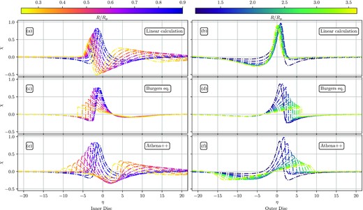
Evolution of the wave profile for a low mass planet, Mp = 0.01Mth. From top to bottom we show azimuthal slices (at several radii) of the planet-driven density perturbation obtained by (panels a–b) solving the linear perturbation equations, (panels c–d) solving Burgers equation and (panels e–f) full non-linear simulation with athena+ +. The left-hand and right-hand rows show inner and outer disc, respectively. As a result of non-linear effects (i.e. as compared to the top row showing the linear results), the wave steepens, shocks and subsequently decays in amplitude (while getting stretched azimuthally). In the inner disc, one can also see the emergence and non-linear steepening of the secondary arm.
Moving to solutions of the Burgers equation (panels c & d), we see that the inner and outer disc evolve very similarly, as expected from the form of the equation. Since this equation does not account for the linear wave evolution, its solutions do not capture the formation of the secondary arm in the inner disc and transfer of flux between the troughs in the outer disc. The non-linear nature of this approximation leads to steady wave steepening that eventually leads to the formation of a shock (a sharp jump in the wave profile). After the shock has formed, the resulting dissipation gradually reduces the wave amplitude while the wave profile broadens.
Comparing the top and bottom rows, we find excellent agreement in both the shape and amplitude of the excited wake close to the planet, confirming that our implementation in athena+ + reproduces the linear prediction for Mp ≪ Mth. But as the distance from the planet increases, the wave profile in a simulation (panels e & f) gets additionally distorted by non-linear effects, leading to a horizontal shift of its peak to more positive (negative) values of η as compared to the linear prediction in the outer (inner) disc. After a shock is formed, the wave starts to decay due to dissipation. Note that far from the planet (R ≳ 2.4) and (R ≲ 0.5), the wakes in panels (e) & (f) do not display such steep jumps as the solutions of Burgers equation, most likely because of wave dispersion (and some numerical diffusion). This comparison clearly shows that the full calculation (bottom row) naturally combines linear and non-linear effects, with both playing important roles.
To further understand the different approximations used in this work, in Fig. 4 we show the rescaled angular momentum flux FJ/FJ, 0 (see equation 6) computed in different ways, as a function of radius R. For the athena+ + simulations and the linear calculation, we compare results for |$F_J^\mathrm{WKB}$| in the WKB approximation (i.e. with FJ obtained from Φ, see equation 13) to FJ obtained directly from the full solutions for density and velocity perturbations, see equation (5). In the case of Burgers equation that has been reduced to the variable χ, we show only the former.7
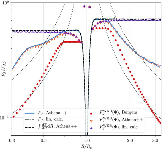
A detailed comparison of different wave angular momentum metrics for Mp = 0.01Mth. We compare the results for FJ obtained using equation (5) (left-hand column in the legend) as well as calculated using the WKB approximation via equation (13) (|$F_J^\mathrm{WKB}$|, right-hand column in the legend). AMFs computed in the linear approximation (Section 3.2) are shown with grey dash-dotted and purple tripod curves; |$F_J^\mathrm{WKB}$| obtained using the solutions to Burgers equation is shown with red dots; FJ and |$F_J^\mathrm{WKB}$| computed using athena+ + models are shown via the blue solid and orange points; the black dashed curve shows the integrated torque. All fluxes are rescaled by the characteristic amplitude FJ, 0. The dotted grey lines indicate the scaling expected for an N-wave, FJ ∝ τ−1/2, with two different normalizations.
In the linear calculation (grey dash-dotted) FJ first increases with |R − Rp| close to the planet, before reaching a plateau a few scale-heights away from the planet. At the same time, the linear |$F_J^\mathrm{WKB}$| disagrees with the corresponding FJ close to the planet. This disagreement is expected, since the wake becomes tightly wound (and WKB approximation becomes accurate) only after propagating a certain distance away from the planet. Beyond ≃ 0.3Rp from the planet, both ways of computing AMF agree to within a few per cent. Note the asymmetry in the saturated FJ levels between the inner and outer discs, that is ultimately responsible for planet migration.
The |$F_J^\mathrm{WKB}$| computed using the solution of Burgers equation (red dots) shows an initially constant flux (which is below the linear prediction since the initial condition for the Burgers evolution was set close to the planet, where the linear FJ has not yet fully accumulated), until the shock is formed ≃ 0.3Rp away from the planet, in good agreement with the predicted shocking distance lsh ≃ 0.27Rp. Beyond that point, the Burgers AMF decays and asymptotically follows the N-wave scaling, FJ ∝ Φ ∝ τ−1/2 (grey dotted curves with different normalization), although convergence to the asymptotic scaling is slow, as expected from GR01 and the fact that τ is small for low Mp, see equation (18).
Finally, for the FJ derived from our simulations (blue solid curve) we find excellent agreement with the linear FJ close to the planet, for |R − Rp| ≲ lsh – the location and amplitude of the peak FJ match precisely. This means that FJ is accurately conserved after excitation, indicating negligible numerical dissipation. To provide yet another check, we plot the integrated torque density from the simulation with the black dotted curve, which agrees perfectly with FJ close to the planet (and with the linear FJ far from it).
At a distance that agrees with the theoretical prediction lsh and results from Burgers equation, the wave in our simulation shocks and starts to decrease. Its FJ drops below the linear FJ and the integrated torque density. At the same time, both in the inner and outer disc, FJ decays notably slower than what Burgers equation predicts. The slow decay in the inner disc between 0.4 ≲ R/Rp ≲ 0.6 can be easily recognized as being caused by the formation of the secondary arm, see Fig. 3. But even in the outer disc, where this effect is absent, the FJ at the damping boundary in the full simulation is still 2–3 times higher than |$F_J^\mathrm{WKB}$| resulting from the Burgers evolution.
4.2 An intermediate mass planet, Mp = 0.25Mth
We now examine the case of a more massive planet Mp = 0.25Mth, keeping the same (fiducial) disc parameters.
In Fig. 5, we again plot azimuthal wake profiles, this time omitting the linear calculation, which is no longer relevant for this Mp because of the increased importance of non-linear effects. As compared to the low-Mp case, we see that the shock forms closer to the planet and the wave evolves faster, e.g. the wake decays and broadens azimuthally more rapidly. This is because equation (18) yields larger values of the time-like coordinate τ for higher Mp, everything else being equal. As expected, solutions of the Burgers equation again differ from the full simulation results by not capturing the formation of the secondary spiral arm in the inner disc, see panels (a) and (c). Also, similar to the low-Mp case shown in Section 4.1, Burgers framework (top row) predicts a stronger wave decay and a slower advance of the shock front compared to the simulation (bottom row) at intermediate distances from the planet (R/Rp ≲ 0.8 and 1.3 ≲ R/Rp). Nevertheless, the evolution of the wake shape in an Mp = 0.25Mth simulation bears more resemblance to the Burgers equation solutions than in the Mp = 0.01Mth case, because of the increased importance of wave non-linearity.
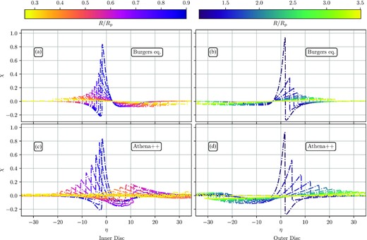
Same as middle and bottom rows of Fig. 3 but for an intermediate-mass planet, Mp = 0.25Mth. Note a faster non-linear evolution of the wave profile.
These conclusions are corroborated by the behaviour of the angular momentum fluxes in Mp = 0.25Mth case, see Fig. 6. In a simulation, shortly after reaching the maximum value that agrees with the integrated torque density, FJ begins to decay as a result of wave shocking at lsh ≃ 0.075Rp away from the planet. The FJ damping is faster for this higher Mp, and the AMF decreases by more than a factor of 10 when the wave reaches the damping zones. In the inner disc, this decay is again delayed by the formation of the secondary arm, but overall, both in the inner and outer discs, FJ is not too deviant from the τ−1/2 scaling expected from the Burgers framework, which is reasonably well followed by the Burgers |$F_J^\mathrm{WKB}$| (red dots). Even though FJ in a simulation still decays with the distance slower than the Burgers |$F_J^\mathrm{WKB}$|, the disagreement between the two is reduced for higher Mp.
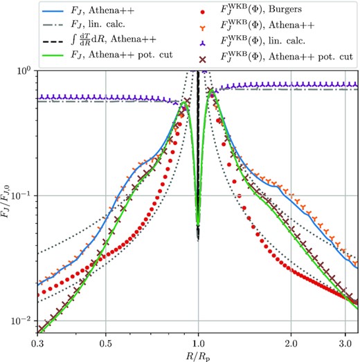
Same as Fig. 4 but for Mp = 0.25Mth. Results from the linear calculation are identical to those presented in Section 4.1 and are shown just for reference. The green curve and brown crosses show the results of an Mp = 0.25Mth run with a spatially truncated potential (see equation 42), discussed in detail in Section 8.1. Note that AMFs show no extended plateau after wave excitation, as for this Mp the shock forms at a distance lsh ≃ 0.075Rp from the planet. The higher amplitude wave leads to a stronger shock, resulting in faster wave decay. See the text for details.
5 CHARACTERISTICS OF THE PLANET-DRIVEN SPIRAL SHOCKS
In agreement with the local version of the non-linear evolution framework (18)–(12), Dong et al. (2011b) found that shocks forming in their simulations as a result of non-linear evolution of planet-driven density waves possess certain universal characteristics. We now examine whether the same is true in our global setup.
5.1 Evolution of the shock strength
The main characteristic of a shock wave is its strength ϵ ≡ ΔΣ/Σ, where ΔΣ is the surface density jump (in 2D) across the shock front. Measuring ϵ in isothermal simulations can be surprisingly difficult (especially for weak shocks), which has been noted before. This issue does not arise for non-isothermal shocks, for which the entropy jump can be used to effectively estimate the shock strength (Arzamasskiy & Rafikov 2018). Previous studies have often used the peak value of the surface density perturbation to determine the shock strength (e.g. Ziampras et al. 2020). This approximation would be reasonable for a density wave that has already evolved into an N-wave. However, it will fail for the waves that are just starting to develop shocked segments.
At the next level of sophistication, one can compare the minimum and maximum values of the density perturbation δΣ/Σ0 inside some azimuthal interval δϕ around the discontinuity. We found that the results of this method depend strongly on the choice of δϕ, which can lead to inconsistent results.
We use this relation in our simulations to find the angular momentum deposition rate due to the shock ∂RFJ|diss as the difference between the radial angular momentum flux divergence and the torque density (equation 4) directly computed from the simulation data (i.e. we use divergences of the Riemann fluxes and the source term monitored in athena+ + on the run). At radii where there is only one shock (i.e. that of the primary arm), the knowledge of ∂RFJ|diss then allows us to deduce the shock-strength ϵ by solving equations (27)–(28) for ϵ, assuming m = 1 and using a Newton–Raphson root finder. We note that this method requires high resolution simulations to ensure that linear damping due to numerical viscosity does not significantly affect ∂RFJ, which would otherwise bias our estimate of ϵ.
We illustrate the application of this procedure to our simulation results in Fig. 7, where we display the shock strength expressed in terms of Δχ – the jump of χ across the shock, which can be related to ϵ via equation (11). We show Δχ as a function of the coordinate τ for several planet masses (increasing from top to bottom) and fiducial disc parameters, for both the inner (blue) and outer (orange) disc. This figure clearly reveals a rather universal evolution of the shock strength: around τ = τsh defined by the equation (15) a shock appears, Δχ becomes non-zero and rapidly reaches its maximum value, after which it gradually falls off, showing a scaling close to that expected from Burgers equation, Δχ ∝ τ−1/2. For all masses, we find that the outer wake produces a stronger shock, consistent with higher wave amplitudes at excitation for the fiducial disc parameters. Comparing Δχ obtained by this method to the jumps in azimuthal profiles of χ in Figs 3, 5, we find good agreement.
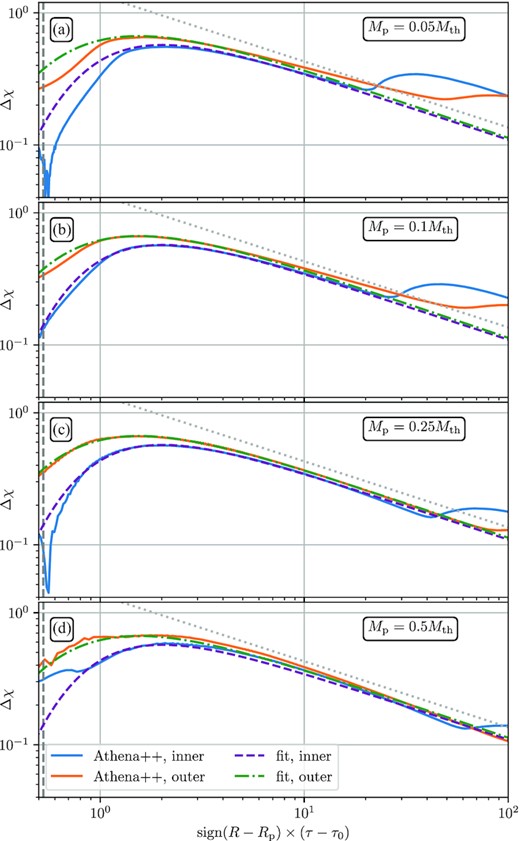
Shock strength Δχ (jump of χ across the shock) obtained from our simulations using a method described in Section 5.1 as a function of the coordinate τ, for different planet masses Mp, and the fiducial disc parameters p = 3/2, h = 0.05. The blue and orange curves show results in the outer and inner disc, respectively. The same value of τ corresponds to different radial separations from the planet, depending on planet mass (see equation 18). As expected from the Burgers equation framework, there is a strong similarity in Δχ(τ) behaviour across all masses. The green dotted and purple dashed lines show a fit (in the outer and inner disc, correspondingly) using a smooth broken two-component power law, see equations (30). The grey dash-dotted lines show the scaling Δχ ∝ τ−1/2 expected for large τ.
Parameters of the fit to Δχ(τ) (see equation 30).
| A | |$\tilde{\tau }_\mathrm{b}$| | α1 | α2 | Δ | |
|---|---|---|---|---|---|
| Inner disc | 2.07 | 0.300 | −10.84 | 0.505 | 0.623 |
| Outer disc | 3.11 | 0.181 | −8.63 | 0.525 | 0.766 |
| A | |$\tilde{\tau }_\mathrm{b}$| | α1 | α2 | Δ | |
|---|---|---|---|---|---|
| Inner disc | 2.07 | 0.300 | −10.84 | 0.505 | 0.623 |
| Outer disc | 3.11 | 0.181 | −8.63 | 0.525 | 0.766 |
Note that for large values of τ in the inner disc, the shock strength inferred from the simulations displays a second peak. It is associated with the emergence of the secondary spiral arm and its evolution into a shock. Since the appearance of a secondary arm is a linear effect (Miranda & Rafikov 2019a), taking place at a fixed distance from the planet, the shift of the second peak towards higher τ for larger Mp can be well understood using equation (18). Once the secondary shock has formed, our fit (30) no longer works in the inner disc.
In the outer disc, the rising Δχ that is seen for large τ at low planet masses (0.05–0.25Mth) is simply due to the fact that the wave reaches the damping zones, making our estimate of the shock strength invalid.
5.2 Location of the shock front
Another important characteristic of a planet-driven density wave is its global shape in the R − ϕ coordinates. Understanding the factors determining the shape of a density wave is crucial for interpreting observations of the spiral arms in protoplanetary discs (e.g. Zhu et al. 2015; Bae & Zhu 2018). Also, as we will show in Section 6, the geometry (curvature) of the spiral shock has direct effect on the generation of vortensity. Here we outline theoretical expectations for the shape of the spiral shock and compare them to simulations.
In linear theory the wave shape (defined as the R − ϕ curve along which η = const.) should be given by ϕ = ϕlin(R), see equation (7). However, non-linear effects cause broadening of the wake, which steadily displaces wake maximum in the azimuthal direction compared to the linear prediction, see Fig. 5 for a clear illustration of this phenomenon (note that η ∝ ϕ − ϕlin).
In our runs the shock front is found by searching for a maximum value of ∂ϕln Σ at a fixed R, a method which has been used before by Arzamasskiy & Rafikov (2018) to locate the wave front as the steepest part of its profile. In the inner disc, care has to be taken at radii where the secondary arm forms and eventually creates a shock. As we have seen in previous sections, both linear and non-linear effects can lead to a shift of the wave front, contributing to Δϕsh in the inner disc. Recall that even for the global linear calculation, the front of the primary wake is not centred at η = 0 (see Fig. 3).
In Fig. 8, we display the global wave pattern in a simulation of the fiducial disc model with Mp = 0.25Mth, and compare it with both linear (equation 7) and non-linear (equation 32) predictions. Around excitation, the linear wake prediction ϕlin (centred on η = 0) is already slightly offset from the wave front (see Figs 3a and b). As the wave propagates away from the planet, the disagreement in ϕ between the ϕlin and the actual position of the shock increases, mainly due to the aforementioned non-linear effects. Additionally, in the inner disc, the secondary arm forms behind the primary at R ≃ 0.6Rp, eventually passing through ϕlin.
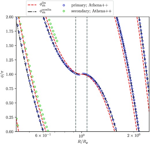
Global pattern of the primary wave front, defined as the steepest part of the azimuthal density profile for the fiducial disc and planet with Mp = 0.25Mth. The blue and green dots mark locations of the primary and secondary arm from the simulation, respectively. The red dashed curve follows the theoretical linear prediction (equation 21) and the black dash-dotted curve is a theoretical fit given by the equations (32) and (33). The radial separation lsh at which the shock forms is marked by vertical dashed lines. See Section 5.2 for details.
In Fig. 9, we plot the azimuthal deviation from the linear prediction Δϕsh found in simulations as a function of τ, for two different planet masses, Mp = 0.05Mth and 0.25Mth. One can see that Δϕsh steadily increases with τ as the non-linear effects accumulate in the course of wave propagation. We fit these numerical results with a behaviour in the form (31), determining the values of the coefficients in front of the scaling as indicated in the legend of Fig. 9(a) (which uses hp = 0.05). We find that in a fiducial disc the value of Δϕ0 fitted to the numerical data varies by only a few per cent as Mp changes from 0.05Mth to 0.5 Mth. The dependence of Δϕ0 on hp or surface density slope is studied in Section 7, and shown to be negligible. This is expected as any dependence on these variables and Mp is already absorbed in the equation (32) and the definition of τ, see equation (18).
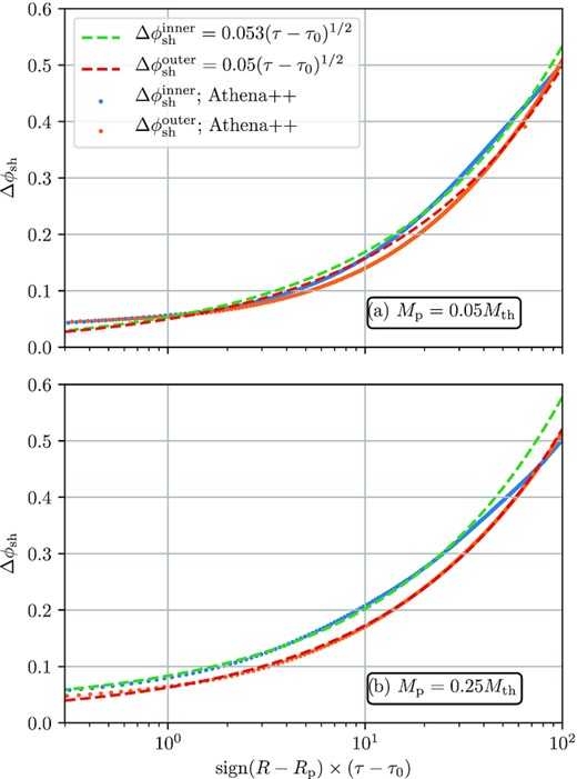
Deviation of the azimuthal shock location from linear theory prediction Δϕ = ϕsh − ϕlin. Simulations results for fiducial disc parameters with Mp = 0.05Mth (top) and Mp = 0.25Mth (bottom) are shown. The blue and orange dots mark simulation results for the outer and inner disc, respectively. A fit for equation (31) is given by the red and green dashed lines, with a proportionality constant indicated in the legend.
The non-linear prediction (32) with thus fixed Δϕ0 is shown as the blue dot-dashed curve in Fig. 8. One can see that it follows the location of the primary arm very well over a significant radial range both in the inner and outer discs. The prescription (32) and (33) will be extensively used in the next section.
6 VORTENSITY EVOLUTION DUE TO PLANET-DRIVEN SHOCKS
Figs 1(c) and (d) shows the vortensity deviation δζ = ζ − ζ0 from its initial value9 ζ0 for a simulation with fiducial disc parameters and Mp = 0.25Mth after 740 planetary orbits. Panel (d) shows a 2D map of δζ and panel (c) a radial profile of the azimuthal average. One can see that close to the planet, the initial vortensity is conserved, i.e. δζ = 0. However, beyond the black-dashed lines marking the radial separation from the planetary orbit at which the wave shocks, |R − Rp| = lsh, the vortensity perturbation δζ becomes non-zero. As fluid parcels pass through the curved shock front (seen in Fig. 1a) at |R − Rp| > lsh, they experience a small jump in vortensity; after one synodic period with respect to the planet they return to a similar position at the shock, experiencing another ζ jump of the same amplitude,10 and so on. Over time, this steady accumulation of small Δζ increments leads to the emergence of an almost axisymmetric vortensity distribution near the planetary orbit, exhibiting maxima (minima) close to (farther from) the planet. Emergence of the second, lower amplitude vortensity peak in the inner disc around R ≃ 0.6Rp (panel c) is due to the shocking of a secondary spiral arms that forms prior to that (panel a).
6.1 Vortensity generation by the global shock
While equation (40) shows similarity to the local expression for Δζ in Dong et al. (2011b), we note that due to the non-linear shear and the more complex shock geometry appearing in the global cylindrical disc, this formula for Δζ does not reduce to an expression in terms of τ alone. However, we can still evaluate this equation numerically for different disc parameters and planet masses and compare the results directly to fully non-linear simulations to verify the analytical prediction (40).
6.2 Semi-analytical model for vortensity production by the planet-driven shock
Results of Section 5 provide us with theoretical expectations for the global behaviour of the shock strength ΔΣ/Σ0 and the shock position as functions of disc parameters and planet mass. Combining them with the calculations in Section 6.1, we can formulate a semi-analytical prescription for vortensity generation by the planet-driven shock, based on the framework of RR02 (see Section 2.3).
Given a set of disc and planet parameters – p, hp, Mp/Mth – this prescription consists of the following sequence of steps:
Use the definition (18) to compute τ(R).
Use the fit equation (30) with parameters in Table 1 to predict shock strength Δχ as a function of τ(R).
Utilize an expression for the shock position ϕsh, which sets C(R), see equation (C5). We will examine two approximations for ϕsh in this work:
Plug the resultant expressions for ϕsh(R) and Δχ(R) into equation (40) to finally obtain the radial profile of the vortensity jump across the shock Δζ(R).
This recipe for calculating Δζ(R) is tested and validated in the rest of the paper.
6.3 Simulation results for vortensity generation in a fiducial disc model
We now turn to vortensity generation observed in our simulations and compare it to the semi-analytical model described above.
In Fig. 10, we display the results for Δζ(R) obtained from our fiducial disc model simulations (blue curves), with Mp/Mth ranging from 0.01 to 1. Radial profiles of Δζ are derived from our non-linear simulations after 20 planet orbits using equation (41) in which we approximate ∂tζ(R) = ∂t〈ζ(R)〉ϕ. The vertical axis is rescaled by the third power of Mp/Mth, to absorb the most important scaling with Mp in equation (40). Radial distance from the planet is rescaled by the shock distance lsh, which is a natural length-scale of the problem in the local limit (GR01). These renormalizations lead to Δζ(R) profiles that have very similar radial shape. However, slight variations are still visible as the planet mass varies, they are discussed below.
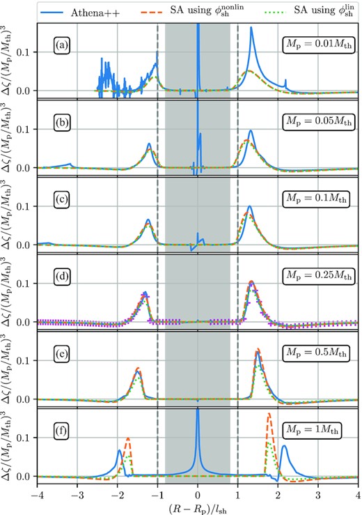
Radial profiles of the vortensity jump across the shock Δζ(R). We compare simulation results (blue) with semi-analytical prediction described in Section 6.2, that use different inputs for the shock location ϕsh: |$\phi _\mathrm{sh}^\mathrm{lin}$| (green dotted) and |$\phi _\mathrm{sh}^\mathrm{nonlin}$| (orange dashed). The dark grey area marks regions where vortensity changes, if present, are not due to the spiral shocks; vertical dashed lines mark |R − Rp| = lsh. Magenta crosses in panel (d) show Δζ computed using equation (40) with inputs for shock position and strength obtained directly from simulations, showing excellent agreement with observed vortensity generation. For more details see Section 6.3.
Before the shock forms, vortensity is mostly conserved, except for numerical artefacts that are amplified for the lowest planet masses. Also, in the coorbital region of the planet we observe the well-known mixing of material on horseshoe orbits (Paardekooper & Papaloizou 2009), homogenizing the vortensity distribution.
As the density wave starts turning into a shock beyond |R − Rp| = lsh (marked by vertical dashed lines), a narrow positive peak in Δζ forms between 1 ≲ |R − Rp|/lsh ≲ 2, followed by a wider but shallower negative trough at larger distances from the planet. The former is due to the rapid formation of the shock and the latter due to its subsequent decay. The overall shape of the Δζ(R) curves is roughly the same in the inner and outer discs, although the outer Δζ peak is higher than the inner one, illustrating the importance of global effects (in the local calculations of Dong et al. (2011b) the peaks are symmetric). Also, at small Mp one can see a low amplitude secondary peak in the inner disc that recedes from the planet (in |R − Rp|/lsh coordinate) as Mp increases. This peak appears due to the shocking of the secondary arm.
Before detailed testing of the prescription outlined in Section 6.2, we checked the validity of the equation (40) by using it to compute Δζ(R) with the main inputs11 obtained directly from our simulations – shock strength Δχ(R) from angular momentum flux decay, equation (27) and shock shape ϕsh(R) – instead of using semi-analytical fits (30), (32), (33). This calculation is illustrated for Mp = 0.25Mp by magenta crosses in Fig. 10(d), providing an excellent match with simulation results and confirming that the shock is the only relevant source of vortensity. This agreement also shows that equation (40) is valid and the code performs as expected.
The green dotted and orange dashed curves in Fig. 10 illustrate the semi-analytical prescriptions for Δζ(R) (described in Section 6.2), computed for ϕsh = ϕlin and |$\phi _\mathrm{sh}=\phi _\mathrm{sh}^\mathrm{nonlin}$|, respectively. By design, these prescriptions agree best with simulation results for 0.1 ≤ Mp/Mth ≤ 0.5, since the parameters (see Table 1) of the fit (30) were determined for Mp = 0.25Mth. The discrepancies at low Mp arise most likely because of the increased importance of linear (validity of the fit for Δχ) and numerical effects for small-amplitude density waves (see the discussion of Fig. 11 below).
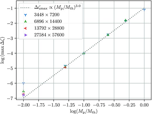
Scaling of the peak value of the vortensity jump Δζ in the outer disc as a function of planet mass for a fiducial disc model. We show results of simulations with several resolutions, which demonstrate that low planet masses require high resolution to show convergence. The dotted line shows the |$\Delta \zeta \propto M_\mathrm{p}^3$| scaling (see equation 40) familiar from the local study of Dong et al. (2011b).
In the highest mass case (Mp = Mth), the agreement with the simulation results is poor, since non-linear effects are strong and the shock forms while the wave is still accumulating angular momentum, in contrast to the assumptions of the GR01 and RR02, see Section 2.3. This spatial overlap of the excitation and propagation regions is also responsible for the shift of vortensity peaks away from |R − Rp| = lsh at high Mp. This is because in the global case the rescaling of radial separation by lsh is not identical to expressing the distance from the planet through the coordinate τ.
Semi-analytical curves computed for the two different approximations for ϕsh (see Section 6.2) differ from each other only for Mp ≳ 0.5Mth. This is expected, since at low masses non-linear effects are weak and |$\phi _\mathrm{sh}^\mathrm{nonlin}\approx \phi _\mathrm{lin}$|. We find that, for practical purposes, using the simple approximation ϕsh = ϕlin for semi-analytical calculation of Δζ(R) is at least not inferior to the more sophisticated assumption |$\phi _\mathrm{sh}=\phi _\mathrm{sh}^\mathrm{nonlin}$|.
Fig. 10 clearly illustrates that over a wide range of planet masses (0.05 − 0.5Mth), vortensity generation exhibits the self-similar behaviour expected in the framework of RR02, as long as the distance from the planet and Δχ amplitude are scaled according to theory. The vortensity amplitude scaling is additionally illustrated in Fig. 11, where we show the peak value of Δζ in the outer disc as a function of planet mass in simulations using the fiducial disc model. One can see a clear power-law behaviour scaling that is well fitted with maxΔζ ∝ (Mp/Mth)3 (dotted line in the figure). This scaling was found in Dong et al. (2011b) in the local (shearing-sheet) approximation, but clearly is valid in the global case as well. This is not surprising since |$\Delta \zeta \propto M_\mathrm{p}^3$| is the dominant dependence on Mp in the global equation (40), with additional Mp-dependent terms playing a minor role.
Fig. 11 also illustrates the numerical convergence of our results over a wider range of resolutions, indicated by different symbols. One can see that convergence is very good, except at the lowest Mp = 0.01Mth, which requires the highest resolution (464 cells per scale-height at the planets orbital radius) to appear converged.
6.4 Effect of gap opening
Up to this point we always assumed the disc surface density near the planet to be unperturbed and vary only on scales of order Rp. However, as the angular momentum lost by the damping density wave is absorbed by the disc fluid, a radial redistribution of gas around the planet’s orbit takes place, eventually resulting in gap opening. This will modify the planet-driven wave in several ways.
First, suppression of the surface density near the planet reduces the strength of its gravitational coupling to the disc, resulting in weaker planetary torque and lowering the density wave amplitude at excitation (Petrovich & Rafikov 2012). Secondly, as the wave propagates across an inhomogeneous background at the gap edge, its non-linear steepening and decay get modified as described in RR02 and Rafikov (2002b). These factors combine to modify vortensity generation by the planet-driven shock.
We illustrate this in Fig. 12 by showing a time-series (over 700 orbits) of azimuthal averages of the vortensity perturbation (panel a), its time-derivative (panel b), and the surface density profile (panel c). Results are shown for the fiducial disc model and Mp = 0.25Mth.
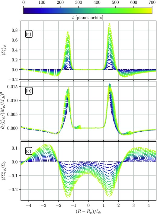
Time series of radial profiles of (a) vortensity perturbation, (b) its time derivative (proportional to Δζ), and (c) surface density perturbation, illustrating the effect of a forming gap. The results are shown for Mp/Mth = 0.25 and the fiducial disc parameters, however using the lowest resolution in order to show evolution over a longer time-scale.
One can see that a characteristic double gap (Rafikov 2002b) slowly grows in depth around the planetary orbit. This process is accompanied by continuous enhancement of the vortensity perturbation, with the positive (negative) δζ(R) associated with reduced (increased) surface density. This steady increase of δζ eventually produces large radial gradients of vortensity near the planet that can lead to non-negligible radial advective transport of vortensity (which we normally find to be unimportant) during gap opening.
At early times, ∂t〈δζ〉ϕ exhibits a very stable, time-independent profile (that we use in Fig. 10). But once gap depth reaches 〈δΣ〉ϕ/Σ0 ≲ 0.15, we find ∂t〈δζ〉ϕ to deviate from the initial smooth profile. At this point, since δΣ is still relatively small, we observe only localized changes of ∂t〈δζ〉ϕ profile: its peak broadens and goes down in amplitude, also showing a small kink around the maximum value (most likely due to vortex formation at late times). On longer time-scales, when the gap gets deeper, we expect vortensity production at the shock to be modified more severely.
7 RESULTS: VARIATION OF THE DISC PARAMETERS
Next we examine how our results and the comparison with semi-analytical calculations change as we vary the underlying disc model. We will predominantly focus on the AMF behaviour and vortensity generation as our metrics for comparison since they provide very sensitive diagnostics of the non-linear wave evolution.
7.1 Variation of the surface density slope
First, we turn to a disc model that has the fiducial value of hp = 0.05 but a constant background surface density, i.e. p = 0, see equation (2). Different from the fiducial disc, this model has a global non-zero vortensity gradient, since its ζ0, K(p = 0) ∝ (R/Rp)−3/2, see equation (36). This may somewhat increase the role of the advective transport of vortensity. Given the generality of the framework outlined in Section 2.3, we expect the effects of a different slope of Σ0(R) on wave evolution to be fully absorbed in the definitions of the coordinates χ and τ.
We begin by presenting in Fig. 13 the behaviour of AMF for a planet of mass Mp = 0.01Mth. Comparing it to Fig. 4, we see very similar behaviour close to the planet: after wave excitation, its AMF reaches values comparable to the fiducial case and begins to decay at a similar distance. Thus, the shocking length lsh is still captured by the equation (17). Moreover, the R − ϕ shape of the wake is still accurately fit by the equations (32) and (33).

However, on the global scale, we see that wave damping is accelerated (slowed down) in the inner (outer) disc. As a consequence less (more) AMF reaches the damping boundary. This is true for the full simulation as well as for the solutions of the Burgers equation and can be directly understood from the effect of p on τ: according to Fig. 2, τ reaches higher (lower) values in the inner (outer) disc, as compared to the fiducial disc. This behaviour is observed across all planet masses. Qualitative differences between evolution described by the full set of hydro equations (athena+ +) and by Burgers equation (see Section 4) still remain.
Next we examine the vortensity generation. Our semi-analytical framework should provide a good match for the ζ production at the shock when p = 0, since all variables in our framework naturally account for arbitrary p. In Fig. 14, we compare simulation results against the semi-analytical model (Section 6.2) for p = 0. The filled grey area marks the corotation region, where the horseshoe flow mixes regions of different initial vortensity advectively. We do not show simulation data in this region as ζ changes there are not due to shocks. First we note that, as opposed to the fiducial disc, the inner peak now dominates over the outer one in the linear regime (Mp/Mth = 0.01). Very importantly, this behaviour is correctly captured by our semi-analytical model (orange dashed curve). For the three higher planet masses (0.1 ≤ Mp/Mth ≤ 0.5), the agreement between our semi-analytical theory and simulations is very good.

7.2 Variation of the disc scale-height
Next we explore the effect of variation of the disc aspect ratio by studying simulations with hp = 0.07 and 0.1. These are performed at the same resolution as the fiducial models that we deem converged, effectively increasing the number of grid cells per scale-height. Thus, simulations at larger hp are expected to be converged too, which we have confirmed.
Variation of hp is expected to have a direct effect on the amplitude of the wave perturbation at excitation. For a fixed planet mass, higher hp results in smaller amplitude of the perturbation (since Mth is higher and Mp/Mth is lower) and the density wave carries less angular momentum, see equation (6). But if we keep Mp/Mth fixed, then the wave amplitude, expressed through χ, remains the same. From equation (18), we also find |$\tau \propto h_\mathrm{p}^{-5/2}$|, meaning that non-linear evolution, expressed via τ-coordinate, is slowed down in hotter discs. In terms of radial distance, this dependence is approximately absorbed in the dependence of lsh on hp, as we demonstrate below. And regarding the R − ϕ shape of the wake (Section 5.2), we find that the linear dependence on hp of the non-linear correction term |$\phi _\mathrm{sh}^\mathrm{nonlin}-\phi _\mathrm{lin}\propto h_\mathrm{p}$| in equation (32) provides an excellent match to the simulation results.
In Fig. 15, we show Δζ as a function of hp (rows) for Mp/Mth = 0.1 (left-hand column) and Mp/Mth = 0.25 (right-hand column). For both masses, the general shape of Δζ is maintained and Δζ curves appear very similar when R − Rp is rescaled by lsh. Thus, our semi-analytical model (Section 6.2) provides a good match to simulation results.
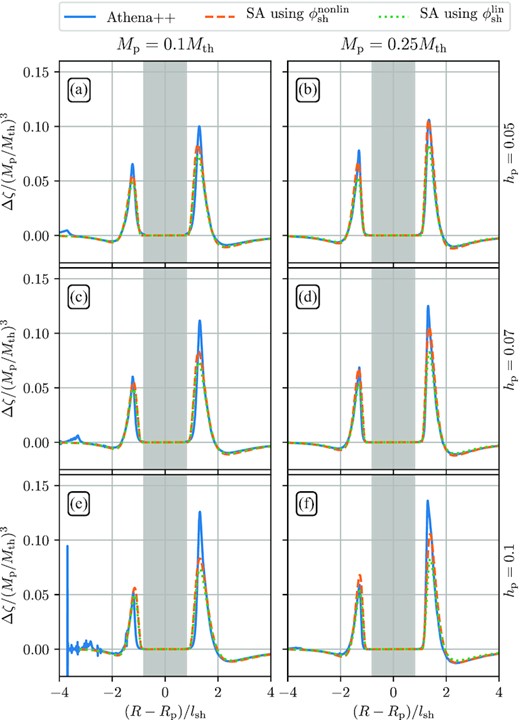
Same as Fig. 10 but now for three values of the disc aspect ratio hp (constant across rows) and two values of Mp/Mth (constant within columns). In the bottom left-hand panel, the inner damping zones and domain boundary lies within 4lsh, which results in somewhat noisy data.
Note that as hp increases, peak values of Δζ increase (decrease) in the outer (inner) disc. We traced this behaviour to the effect of hp on the initial (linear) wake profile: for higher hp we find the magnitude of minimum and maximum values of χ to increase (decrease) in the outer (inner) disc. But the main effect of changing hp is the variation of the spatial scale of the problem. Since the rescaled (horizontally, by lsh ∝ hp) profiles of Δζ in Fig. 15 remain largely unchanged, this implies that in physical space (in R − Rp) the vortensity profile is broader for higher hp, see Fig. 16 for illustration.
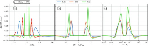
Semi-analytical predictions for vortensity jump in inner and outer disc (solid lines) for a disc with p = 1 and hp = 0.05. We show results for three values of Mp/Mth, as functions of the different coordinates: orbital stellocentric radius (panel a), distance from the planet normalized by lsh (panel b), and the coordinate τ − τ0 (panel c). In panel (a), we additionally show results from a simulation for Mp/Mth = 0.05 (red dot-dashed curve), which confirms that the Δζ peaks in the inner and outer disc are of almost equal height for these disc and planet parameters, as predicted by our semi-analytical model (see Section 8.2 for details).
8 DISCUSSION
The main goals of this work were to numerically verify the semi-analytical theory of planet-driven density wave propagation advanced in RR02, and to explore the impact of the emergence of secondary (and higher order) spiral arm on wave evolution in the inner disc. Using high-resolution athena+ + simulations we were able to confirm the main predictions of the semi-analytical framework of RR02 summarized in Section 2.3.
In particular, we find that the change of coordinates from R, ϕ, Σ − Σ0 to τ, η, χ works very well when describing the planet-driven density wave evolution, as long as certain problem-specific inputs are properly calibrated using simulations. Examples of this include the scaling of |$\phi _\mathrm{sh}^\mathrm{nonlin}-\phi _\mathrm{lin}$| with hp and τ (see equation 32 in Section 5.2), self-similarity of the shock strength profile (see equation 30 in Section 5.1), semi-analytical calculation of the vortensity production in Section 6.2, and so on. In agreement with the findings of Dong et al. (2011b) and Duffell & MacFadyen (2012), we find very good agreement between the theoretically predicted shocking distance lsh (see equation 17) and our global simulation results, even though lsh was derived in GR01 in the local (shearing sheet) approximation. The evolution of the density wave profile towards the N-wave shape is also reproduced in our simulations, see Figs 3 and 5.
Using vortensity generation as a metric, the best agreement between the (calibrated) theory and simulations is found for intermediate planet masses Mp ≃ 0.05 − 0.5Mth. At higher masses approaching Mth the agreement worsens (see Fig. 10f), since the planet-driven wave is non-linear already at excitation and the key theoretical assumption of spatial separation between linear excitation and non-linear propagation breaks down. At low Mp < 0.05Mth, numerical effects as well as the proximity of the wave damping zones (because of the increased lsh, see equation 17), also worsen the agreement with theory, see Fig. 10(a).
The emergence of the secondary spiral arm in the inner disc certainly affects the performance of the RR02 theory, which did not take this subtle linear effect into account. In the inner disc, and especially at low Mp, that theory (as well as its local analogue, see GR01) misses the appearance of a second bump in the profile of Δχ at the shock as a function of τ (see Fig. 7), slow decay of the AMF FJ in the inner disc (see Fig. 4), and secondary peaks of vortensity production (see Fig. 10). For these reasons, in the inner disc the semi-analytical framework of RR02 is valid only for R ≳ (0.5 − 0.6)Rp, before the secondary arm fully forms.
8.1 Validity of Burgers equation for describing evolution of planet-driven density waves
While, as described above, many predictions of the semi-analytical theory of RR02 work very well, once properly calibrated by simulations, some other aspects of theory, starting from first principles, show only qualitative agreement in many cases. In particular, when we attempt to reproduce wave evolution by directly solving the Burgers equation (rather than using simulations to calibrate semi-analytical prescriptions), we find quantitative differences with the simulations. They can be clearly seen in Fig. 3, which reveals a faster decay and slower azimuthal spreading of the density wave profile evolved using Burgers equation (12), as compared to the simulation results, for a low mass planet. Unsurprisingly, this leads to a considerably faster decay of the Burgers |$F_J^\mathrm{WKB}$| compared to both FJ and |$F_J^\mathrm{WKB}$| in simulations, see Fig. 4.
This may seem surprising given that the Burgers equation (12) uses the simulated wake profile near the planet as a starting point for its subsequent evolution. This implies that Burgers equation is not capturing well some wave propagation physics that takes place in the actual simulation. We believe that, at least partly, this missing ingredient is the continued injection of the angular momentum into the density wave by the planetary potential happening in simulations far from the planet, outside of the nominal excitation region. Since the wave amplitude decays due to its dissipation at the shock, addition of even a small amount of angular momentum to the wave far from the planet can significantly slow down the decay of FJ in simulations. By design, this injection is absent in the Burgers equation approach, resulting in the discrepant |$F_J^\mathrm{WKB}$|. An indirect support for this possibility can be seen in the less discrepant |$F_J^\mathrm{WKB}$| for higher Mp = 0.25Mth planet, see Fig. 6: due to faster decay of the wave amplitude in the higher Mp simulation, less angular momentum gets added to the wave far from the planet by its torque.
The AMF behaviour resulting in this run is shown in Fig. 6 via green solid curve (FJ) and brown crosses (|$F_J^\mathrm{WKB}$|), see the legend. One can see that around excitation, the original simulation and the one with truncated potential predict very similar AMF behaviour. But further out, the AMF for a truncated potential decays faster than for the non-truncated Φp, which can be seen by comparing blue and green curves. Both FJ and |$F_J^\mathrm{WKB}$| for a truncated potential stay closer to the Burgers |$F_J^\mathrm{WKB}$| (red points). This provides support to our hypothesis that it is the distant gravitational coupling of the density wave to the planetary potential, that causes the Burgers equation to overpredict the wave decay. On the other hand, the green curve does not fully converge to the red points, which suggests that some other factors may also be at play.
To summarize, while the Burgers equation (12) provides a useful framework for understanding the planet-driven wave evolution at the qualitative level, a more accurate approach (e.g. a theory calibrated by simulations) is needed for quantitative agreement with simulations. This can be important for certain applications, see Bollati et al. (2021) and Section 8.6.
8.2 Vortensity generation at the shock and its semi-analytical description
Our derivations in Section 6.2 and Appendix C provide a natural generalization of the local (i.e. shearing sheet geometry) calculation of the vortensity production in Dong et al. (2011b) to the case of a global (i.e. polar) disc geometry with radial gradients of Σ. Our calculation of the vortensity generation at the shock can also naturally account for the modification of the global shape of the spiral shock by the non-linear effects (Section 5.2), although we find the resulting corrections to be significant only for high Mp, see Section 6.3 and Fig. 10.
This calculation provides a basis for the semi-analytical framework for predicting the vortensity production at the shock, described in Section 6.2. This framework employs a single input – the jump of the dimensionless wave perturbation Δχ at the shock – that is calibrated using simulations. This calibration step yields an accurate description of Δζ(R), that compares very well against simulations, see Sections 6.3 and 7. This, in particular, implies that the radial transport of vortensity has negligible effect on its evolution in the vicinity of the planet, i.e. the variation of ζ can be explained entirely through its production by the planet-driven shock.
The semi-analytical framework for vortensity production is one of the main results of our work and will be used in future calculations of the planet-induced vortensity evolution. Its accuracy allows us to make inferences about the vortensity evolution without running computationally expensive hydrodynamical simulations.
For example, we used this framework to determine the value of the surface density slope p at which the height of the vortensity peaks in the inner and outer disc would be the same; this question is relevant for determining the side of the disc in which vortices triggered by the planetary perturbation might first appear (Cimerman & Rafikov, in preparation). Our semi-analytical approach allows a very efficient exploration of this problem. Given that we previously found the inner (outer) peak of Δζ to dominate for p = 0 (p = 3/2), one should expect the transition (equal amplitude of the vortensity peaks) to take place for some p in the interval (0, 3/2). However, it turns out that the value of p at which this transition takes place also depends on the planet mass. We demonstrate this in Fig. 16 where we display several semi-analytical Δζ(R) profiles computed for p = 1, for three values of Mp and as functions of different coordinates: R/Rp, (R − Rp)/lsh and τ(R). One can see that for this value of p the inner peak dominates for low Mp (blue curve), while for high Mp the outer vortensity peak is higher (green curve). Our theory predicts that Δζ peaks should be almost equal in amplitude for Mp = 0.05Mth. And indeed, in panel (a), we also show data from a simulation run for Mp = 0.05Mth and p = 1 (red dashed) that agrees very well with this theoretical prediction (orange solid).
This figure conveniently illustrates several other important points about the vortensity evolution: scaling of Δζ with Mp, (almost) self-similar appearance of Δζ when expressed in τ(R) and (R − Rp)/lsh coordinates, and the increase of radial scale of Δζ variation as Mp is decreased, see panel (a).
8.3 Effect of equation of state and disc thermodynamics
Our calculations are restricted to globally isothermal discs. At the next level of sophistication, one might wonder what changes would be brought in by considering e.g. the locally isothermal EoS, in which cs is a function of R. We expect two modifications to be introduced by this EoS.
Secondly, the behaviour of ΔΣ is different in locally and globally isothermal discs. Part of the variation comes from the explicit difference in temperature profiles near the planet, but there is also a more subtle contribution. As shown in Miranda & Rafikov (2019b), angular momentum of the density waves propagating in locally isothermal discs is not conserved, unlike in globally isothermal ones. Instead, it scales with the local disc temperature, i.e. |$\propto c_s^2$|, as a result of additional coupling with the background flow (manifesting itself even in the linear regime). This translates into a different behaviour of ΔΣ(R) compared to the discs considered in this work.
We have explored evolution of the wave angular momentum flux in a locally isothermal disc using fargo3d and athena+ +. We found that, especially for sub-Mth planets, wave damping is accelerated or slowed down substantially, beyond the expected effect of changing τ, in agreement with the findings of Miranda & Rafikov (2019b). This changes the ΔΣ and Δχ(R) behaviour in a way that is not obviously generalizable within our current framework. The same is true in the even more general case of a disc with explicit heating/cooling, in which angular momentum flux of planet-driven density waves is known to not be conserved in general (Miranda & Rafikov 2020a, b; Zhang & Zhu 2020).
8.4 Limitations of this work
Our work necessarily employs a number of simplifications, in addition to the ones regarding disc thermodynamics (Section 8.3). One of them is our assumption that the planet-driven density waves decay only as a result of irreversible dissipation at the shock, into which they evolve due to non-linear effects. In real discs there are other, linear, mechanisms that can be responsible for wave damping. In particular, radiative damping has been demonstrated recently (Miranda & Rafikov 2020a) to play a strong role in wave dissipation in protoplanetary discs. Especially for lower mass planets, radiative losses can easily dominate wave dissipation compared to the non-linear damping at the shock (Miranda & Rafikov 2020b). While accounting for the radiative wave damping is possible in principle, as described in Miranda & Rafikov (2020a, b), in practice this procedure may be too cumbersome, leaving direct simulations with explicit heating/cooling as a better option.
We have also neglected the effects of viscosity in our study. While viscous damping of density waves is typically subdominant compared to either linear radiative or non-linear effects (Miranda & Rafikov 2020b), viscosity can smooth out the emerging density gradients and affect the vortensity evolution. However, recent studies (Flaherty et al. 2017, 2018, 2020; Rafikov 2017) have shown that effective viscosities in protoplanetary discs are likely low.
We also neglected the possibility of planet migration, which should result from the asymmetry of the torques exerted by the planet on the disc. Migration can produce additional asymmetry of the surface density and torque distribution around the planet (Rafikov 2002b). In this regard, our results should still be valid on time-scales over which the planet would not migrate significantly.
Finally, our 2D study neglects the possibility of vertical motions in the disc and other related 3D effects. However, previously Zhu et al. (2015) have shown that many aspects of the density wave propagation in 2D discs, including the non-linear effects, directly translate into fully 3D discs (see next).
8.5 Comparison to previous work
Some aspects of the non-linear density wave evolution have been studied numerically in the past. In particular, Duffell & MacFadyen (2012) looked at some properties of the global planet-driven spiral arms using high-resolution 2D simulations. We find good qualitative agreement with the behaviour they reported for FJ derived the WKB approximation, see equations (13) and (14). Comparing our lowest mass case (Mp/Mth = 0.01) to theirs (Mp/Mth = 0.0209), we find very good agreement in the inner disc, including the effect of the secondary arm formation on FJ, which is now well understood. In the outer disc, our results show a slower than FJ ∝ τ−1/2 decay with τ, whereas Duffell & MacFadyen (2012) find a behaviour close to this scaling. We speculate that his might be due to a different implementation of the wave damping at the outer boundary.
Using local (shearing sheet) simulations, Dong et al. (2011b) studied vortensity excitation at the planet-driven shock. Their results for Δζ(R) are compatible with ours regarding the amplitude of the vortensity jump and its radial structure. Their predicted scaling of Δζ ∝ (Mp/Mth)3 is also consistent with our findings. In our global calculations, we find that the amplitude of Δζ can sometimes differ by a factor of ≃ 2–3 between the inner and outer disc in the most extreme cases, which was not possible for Dong et al. (2011b) to observe due to the symmetry of the shearing sheet setup.
Both Dong et al. (2011b) and Duffell & MacFadyen (2012) found that the azimuthal width of the wake evolves as Δη ∝ τ1/2, translating into a similarly behaving offset of the peak position of the non-linear wake from the linear prediction (7), in agreement with our findings, see Section 5.2. Moreover, in their 3D simulations of more massive planets embedded in discs Zhu et al. (2015) also found good agreement of the wake offset with this scaling.
8.6 Applications of our results
Semi-analytical framework for characterizing global planet-driven shocks (Rafikov 2002a), further developed and tested in this study, can be applied to improve understanding of various aspects of disc–planet interaction. For example, our results on the shock strength (Section 5.1) can be used to compute the contribution of the planet-driven shock heating (Rafikov 2016) to thermal balance of the disc; they can also be used for computing the associated mass accretion rate |$\dot{M}(R)$| through the disc. Our semi-analytical fit for the offset between the non-linear shock location and ϕlin, see equation (32) in Section 5.2, can be employed for inferring planet masses from the shapes of spirals observed in protoplanetary discs.
Recently Bollati et al. (2021) applied the non-linear framework of GR01 and RR02 to model kinematic signatures (’kinks’) of planets embedded in the disc, that have been recently observed by ALMA (Pinte et al. 2018, 2019). They used a procedure identical to the one used in making Figs 3(c) and (d) – numerical solution of the Burgers equation (12) with initial conditions from linear theory – to compute the velocity perturbation in the disc due to a planet-driven density wave and to obtain the CO emission channel maps. Although we did not compute a kinematic signature in this work, our results (Section 8.1) suggest that an approach based on solving Burgers equation may easily overestimate wave decay and underestimate the resultant velocity perturbation and the amplitude of a kink.
While the weakly non-linear theory of RR02 strictly applies only to the low planet mass regime, some of its ingredients may be useful also for describing the high-mass (Mp ≳ Mth) regime, relevant for the existing protoplanetary disc observations in CO emission and scattered light. In particular, we expect that, when expressed in terms of the generalized coordinates (8)–(11), the wave properties would still show a universal behaviour even for high Mp, which could be calibrated using simulations.
Our results on vortensity generation (Section 6) can be used for understanding the appearance of vortices in planetary vicinity (Koller, Li & Lin 2003; Li et al. 2005; de Val-Borro et al. 2007). They can also be employed to (semi-analytically) generate axisymmetric surface density profiles for the planet-induced gaps as a function of time, disc parameters and planet mass, following the recipe of Lin & Papaloizou (2010). These applications will be explored in a forthcoming work (Cimerman & Rafikov, in preparation). Finally, our results can be useful for benchmarking the codes used for studying disc–planet interaction, especially through diagnostics such as the angular momentum flux evolution and vortensity production at the shock.
9 SUMMARY
We have studied the non-linear evolution of density waves excited by planets embedded in inviscid, isothermal 2D cylindrical discs with the goal of verifying the weakly non-linear theory of global density waves developed in Rafikov (2002a). Using linear calculations, weakly non-linear theory and full hydrodynamical simulations with athena+ + we explored models for a variety of disc parameters, such as disc scale-heights and surface density slopes, and planet masses spanning two orders of magnitude Mp = (0.01 − 1)Mth. Our findings can be briefly summarized as follows.
The semi-analytical framework of Rafikov (2002a) using rescaled variables τ, η, χ (equations 8–11) provides an accurate description of the non-linear evolution of the global density waves driven by the subthermal mass planets, provided that it is properly calibrated using numerical simulations. In particular, many characteristics of the wave exhibit a behaviour close to self-similar when expressed in terms of these variables.
We showed that calculation of the density wave properties using Burgers equation (12), while qualitatively correct, does not provide a quantitatively accurate description of the wave evolution, in particular, overpredicting wave decay, especially for low planet masses. A better approach would be to rely on numerical calibration of the key inputs of the semi-analytical framework: the global shape of the density wave (equations 32–33), accounting for the non-linear effects, and the strength of the shock into which the wave ultimately evolves (equation 30 and Table 1).
We derive analytical expressions for the vortensity jump across the global planet-driven shock and verify them using numerical simulations (Section 6). We confirm that vortensity generation at the shock scales as a high power of the planet mass, Δζ ∝ (Mp/Mth)3.
Applicability of the weakly non-linear theory (Rafikov 2002a) in the disc interior to the planetary orbit is limited by the emergence of secondary spiral arms, which is a linear effect (Bae & Zhu 2018; Miranda & Rafikov 2019a).
Our results have implications for understanding the appearance of planet-driven spiral arms in protoplanetary discs, kinematic signatures of embedded planets (’kinks’), and other phenomena.
Future work will apply the semi-analytical approach explored in this study to other problems in the area of disc–planet interaction, in particular, the formation of vortices at the edges of planetary gaps driven by the Rossby Wave Instability.
ACKNOWLEDGEMENTS
Software:numpy (Harris et al. 2020), scipy (Virtanen et al. 2020), ipython (Perez & Granger 2007), matplotlib (Hunter 2007), athena+ + (Stone et al. 2020), fargo3d (Benítez-Llambay & Masset 2016) and astropy (Astropy Collaboration 2013, 2018).
We thank the anonymous referee for helpful suggestions, especially in clarifying our explanation of multiple spiral arm formation in the linear case. We are indebted to Ryan Miranda for many useful exchanges and for sharing his method and code to calculate global linear modes, which greatly enriched this work. We would also like to thank all developers of athena+ + for sharing their code with us and in particular Tomohiro Ono, James Stone, and Matt Coleman for helpful discussions. NPC is funded by an Isaac Newton Studentship and a Science and Technology Facilities Council (STFC) studentship. RRR acknowledges financial support through the NASA grant 15-XRP15-2-0139, John N. Bahcall Fellowship, and STFC grant ST/T00049X/1. A large part of the lower resolution simulations were performed on FAWCETT the HPC cluster at DAMTP, University of Cambridge. Special thanks to Kacper Kornet and Deryck Thake for all the support in using local resources. Part of this work was performed using resources provided by the Cambridge Service for Data Driven Discovery (CSD3) operated by the University of Cambridge Research Computing Service (www.csd3.cam.ac.uk), provided by Dell EMC and Intel using Tier-2 funding from the Engineering and Physical Sciences Research Council (capital grant EP/P020259/1), and DiRAC funding from the Science and Technology Facilities Council (www.dirac.ac.uk).
DATA AVAILABILITY
The data underlying this article will be shared on reasonable request to the corresponding author.
Footnotes
We renamed the parameter t from RR02 to τ to avoid confusion with time t, which we use e.g. in the hydrodynamic equations. We also added a sign function that changes from inside to outside the planet’s orbit, such that equation (12) is valid in both regions. This is due to the characteristics changing roles at this point (see GR01).
We use the assumption Ω(R) = ΩK(R) in order to keep the analytical form of the coordinates simpler. We checked that accounting for sub-Keplerian rotation results in negligible changes for thin discs.
athena+ + is publicly available on GitHub.
As noted by Miranda & Rafikov (2019a), the indirect term is linear in R, thus becoming more important for R ≫ Rp. It might be more significant when considering even larger domains of the disc.
These simulations used a total of 8192 threads, distributed over 32 nodes hosting Intel® Xeon PhiTM, running 256 threads each.
The divergent behaviour of Φ around R = Rp is due to the fact that the atmosphere of the planet leads to a finite surface density perturbation there, while g(R) in the definition (11) of χ diverges as R → Rp.
Note that ζ0(R) is slightly different from ζ0, K due to the modification of the Ω profile by the radial pressure gradient.
We comment on long-term evolution and corrections to this simplifying assumption in Section 6.4.
We use a polynomial spline fit over a few cells in order to approximate the numerical parameters of the shock, which is needed to reduce the noise in computation of ∂S(ΔΣ/Σ).
REFERENCES
APPENDIX A: EFFECT OF THE FORM OF SMOOTHED POTENTIAL
The effect on the wave can be seen by examining the wave profile close to the planet. In Fig. A1, we show azimuthal wave profiles for the fiducial disc and Mp = 0.01Mth at R = 1.068Rp and R = 0.935Rp. The same smoothing parameter of the gravitational potential, ϵ = 0.6 (typical in the literature; Müller et al. 2012), is used for both potentials.

We find that |$\Phi _\mathrm{p}^{(2)}$| results in a wave amplitude that is about 25 per cent smaller than when using |$\Phi _\mathrm{p}^{(4)}$|. This is consistent with the observations of Dong et al. (2011b), who found that the second-order potential creates a shock further from the planet, that is weaker, than |$\Phi _\mathrm{p}^{(4)}$|. Indeed, as non-linear effects directly depend on the wave amplitude it is clear that the change of the wave amplitude due to a different potential must affect the time it takes for characteristic to first cross and a shock to be formed. These differences are expected to reduce as the smoothing parameter ϵ is decreased.
APPENDIX B: COMPARISON WITH ANOTHER HYDRO CODE
To test the sensitivity of our results to numerical scheme we also run fargo3d simulations in order to make a direct comparison with athena+ +. We performed simulations at the highest resolution we could achieve on one GPU, NR × Nϕ = 6896 × 14 400, covering the same domain using the same grid structure, damping zones, and boundary conditions as the athena+ + models. For this comparison, we set |$\Phi _\mathrm{p}=\Phi _\mathrm{p}^{(4)}$| (equation 24), used the fiducial disc parameters (q = 1.5; hp = 0.05), and show results for Mp = 0.25Mth. The behaviour of AMF obtained by both codes is displayed in Fig. B1. In all regions of the disc we find very good agreement between the two codes. The small disagreement at a few per cent level might be due to the lower resolution of fargo3d runs.
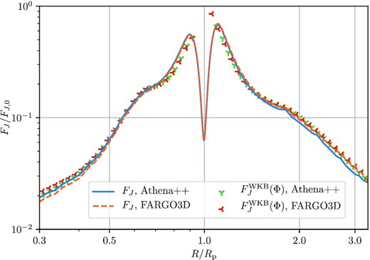
Comparison of the wave angular momentum fluxes – curves for FJ, dots for |$F_J^\mathrm{WKB}$|, as shown in the legend – computed with athena+ + and fargo3d. Calculation is performed for the same parameters as in Fig. 6.
APPENDIX C: DERIVATION OF THE VORTENSITY JUMP
Author notes
John N. Bahcall Fellow at the IAS.
