


ABSTRACT
New multicolour photometric observations were carried out on 22 nights in three observation missions between 2015 October and 2016 February for eclipsing binary HIP 7666. High- and low-resolution spectroscopic observations were also carried out in the winters of 2015, 2016, and 2019, respectively. The fully phase-covered light curves and radial velocity curves are presented. All times of light minima are used to calculate the orbital period [2.372 2200(4) d] and new ephemerides. The photometric solution and stellar physical parameters are derived, showing that HIP 7666 is a detached binary with the absolute parameters M1 = 1.53(3) M⊙, R1 = 2.08(2) R⊙, log L1/L⊙ = 0.99(3), log g1 = 3.98(2), Mbol1 = 2.26(8), Teff,1 = 7100(100) K for the primary, and M2 = 1.23(3) M⊙, R2 = 1.06(2) R⊙, log L2/L⊙ = 0.13(4), log g2 = 4.47(2), Mbol2 = 4.4(1), Teff,2 = 6029(67) K for the secondary. The age of 1.69 Gyr and 1.755 Gyr are estimated from parsec isochrones and mesa evolutionary tracks, respectively. In Herzsprung–Russell (H–R) diagram, the primary component has evolved to the late stages, while the secondary still locates at the early stages of the main sequence. Frequency analysis yields three frequencies of f1 = 24.631(4) cd−1, f2 = 21.193(1) cd−1, and f3 = 28.07(7) cd−1. Comparisons between models and observations suggest that the primary component is most likely a p-mode non-radial δ Scuti oscillator.
1 INTRODUCTION
The contribution of binary stars, especially eclipsing binaries (EBs), to astrophysics can never be overemphasized. The EBs can provide essential information about their components, such as mass, radius, luminosity, etc. In general, these physical parameters of the stars in binary systems can be precisely determined based on photometric and spectroscopic observations. As far as the EBs with pulsating component stars, stellar physical parameters may help to build appropriate stellar models, which provide chances to pick out correct models by comparing the theoretical frequencies with the observation-determined ones hence derive precisely stellar parameters and identify pulsation modes.
Since early 1970s (Tempesti 1971; Broglia & Marin 1974; McInally & Austin 1977), astronomers have noticed that stellar pulsations existed in EBs. However, very few such objects had been observed before 2000. A large number pulsating EBs have been discovered in past two decades, especially those contributed by space missions such as CoRot, Kepler, and TESS (Damiani et al. 2010; Southworth et al. 2011; Maceroni et al. 2013; Guo et al. 2019; Lee, Kristiansen & Hong 2019; Chen et al. 2020). Those EBs containing δ Scuti stars have become research foci with nearly 300 such systems announced (Zhou 2010; Soydugan et al. 2011; Liakos et al. 2012; Liakos & Niarchos 2017; Gaulme & Guzik 2019).
δ Scuti stars are on or above the main sequence in the Herzsprung–Russell (H–R) diagram, and situated in the lower classical instability strip (Breger 2000). They are typically late-A to early-F spectral type stars with a mass of 1.5–2.5 M⊙, and pulsating periods between 0.02 and 0.25 d. These stars typically pulsate in radial and non-radial modes with amplitudes less than 0.3 mag. The oscillations of those stars are mainly driven by κ mechanism that occurs in the partial ionization zone of He ii (Gautschy & Saio 1995; Breger 2000).
The pulsating EB star HIP 7666 (α2000 = 01h38m41|${_{.}^{\rm s}}$|67, δ2000 = + 52o31′07|${_{.}^{\prime\prime}}$|67) was discovered by Hipparcos mission (ESA 1997), and classified as an unknown variable type. Oja (1985) preformed time-series observations of this target and determined its V magnitude, (B–V) and (U–B) colour indices. It was later identified as an EB in the Grup d′Estudis Astron|$\grave{o}$|mics observing program, which was a survey for new variable stars. Escolà-Sirisi et al. (2005) carried out photometric observations between 2000 July and 2000 November and found that it was a detached EB system with the orbital period of 2.372 29(8) d. It was also pointed out that one of the components experienced short-period oscillations with a main pulsation frequency of 24.46 cd−1 or 25.47 cd−1. However, the absolute parameters of this binary system were not given in their work, especially the effective temperature Teff, inclination i, and mass ratio q. The frequency analysis result was also not conclusive because of the low S/N of data. Further multicolour photometric observations are needed, high- and low-resolution spectroscopic observations could be helpful to reveal the nature of the binary system. Therefore, the new photometric and spectroscopic observations of HIP 7666 were performed in 2015, 2016, 2019, and 2020, and described in Section 2. Sections 3 and 4 present the binary solution and pulsation analysis, respectively. The summary and discussion of this work is given in Section 5.
2 OBSERVATIONS AND DATA REDUCTION
2.1 Photometry
A multisite photometric observation run for HIP 7666 was carried out from 2015 October to February 2016. All observations were made through filters in Jonson B, V, and R bands. Most data were obtained with the Nanshan One-meter Wide-field Telescope (NOWT) at the Nanshan Station (Song et al. 2016; Ma et al. 2018; Bai et al. 2020) of Xinjiang Astronomical Observatory (XAO), and also with the 85-cm telescope (XL85cm) at the Xinglong Station (Bai et al. 2018) of National Astronomical Observatories (NAOC). Some additional observations were collected with the 84-cm telescope (SPM84cm) at the Observatorio Astronómico Nacional on the Sierra San Pedro M|$\acute{a}$|rtir (OAN-SPM) in México. The information about these three telescope systems are listed in Table 1. In total, over 130 ∼h with more than 15 000 images of useful data were obtained on 22 nights. The summary and journal of the observations are listed in Table 2.
Informations of the telescopes used for photometric observations.
| Telescope | F/# | CCD | Pixel | Pixel-size | FOV | Image scale |
|---|---|---|---|---|---|---|
| NOWT, (1.0-m) | F/2.2 | E2V-203-82 | 4K × 4K | 12 |$\mu$|m | 1.3° × 1.3° | 1.125 arcsec pix−1 |
| XL85cm | F/3.5 | Andor-DZ-936 | 2K × 2K | 13.5 |$\mu$|m | 32 arcmin × 32 arcmin | 0.934 arcsec pix−1 |
| SPM84cm | F/15 | E2V-4240 | 1K × 1K | 13.5 |$\mu$|m | 7.5 arcmin × 7.5 arcmin | 0.442 arcsec pix−1 |
Journal of CCD photometric observations for HIP 7666.
| Date | Observatories | Telescopes | Filters | Frames | Photometric precision (mag) |
|---|---|---|---|---|---|
| 2015 Oct.11 | NAOC | XL85cm | B,V,R | 182,182,181 | 0.011, 0.015, 0.016 |
| 2015 Oct.12 | NAOC | XL85cm | B,V,R | 217,217,217 | 0.01, 0.011, 0.011 |
| 2015 Oct.13 | NAOC | XL85cm | B,V,R | 123,122,122 | 0.005, 0.013, 0.013 |
| 2015 Oct.14 | NAOC | XL85cm | B,V,R | 342,342,342 | 0.026, 0.037, 0.029 |
| 2015 Oct.15 | NAOC | XL85cm | B,V,R | 371,371,371 | 0.033, 0.04, 0.037 |
| 2015 Oct.17 | XAO | NOWT | B,V,R | 291,287,283 | 0.006, 0.005, 0.006 |
| 2015 Oct.21 | XAO | NOWT | B,V,R | 346,342,342 | 0.014, 0.010, 0.022 |
| 2015 Oct.22 | XAO | NOWT | B,V,R | 148,149,150 | 0.005, 0.012, 0.008 |
| 2015 Oct.24 | XAO | NOWT | B,V,R | 215,206,214 | 0.008, 0.006, 0.008 |
| 2015 Oct.25 | XAO | NOWT | B,V,R | 105,124,131 | 0.004, 0.008, 0.004 |
| 2015 Nov.26 | SPM | SPM84cm | B,V,R | 33, 31, 31 | 0.008, 0.005, 0.004 |
| 2015 Nov.27 | SPM | SPM84cm | B,V,R | 289, 288, 290 | 0.006, 0.005, 0.008 |
| 2015 Nov.28 | SPM | SPM84cm | B,V,R | 187, 188, 190 | 0.007, 0.006, 0.006 |
| 2015 Nov.29 | NAOC | XL85cm | B,V,R | 629, 628, 628 | 0.007, 0.007, 0.009 |
| 2015 Nov.30 | NAOC | XL85cm | B,V,R | 238, 238, 238 | 0.005, 0.005, 0.004 |
| 2016 Jan.01 | XAO | NOWT | B,V,R | 271, 268, 262 | 0.008, 0.01, 0.01 |
| 2016 Jan.02 | XAO | NOWT | B,V,R | 237, 233, 229 | 0.008, 0.008, 0.009 |
| 2016 Jan.03 | XAO | NOWT | B,V,R | 271, 268, 262 | 0.010, 0.012, 0.009 |
| 2016 Jan.04 | XAO | NOWT | B,V,R | 170, 170, 167 | 0.011, 0.008, 0.007 |
| 2016 Jan.06 | XAO | NOWT | B,V,R | 215, 214, 215 | 0.007, 0.008, 0.007 |
| 2016 Jan.16 | XAO | NOWT | B,V,R | 156, 157, 157 | 0.010, 0.012, 0.009 |
| 2016 Feb.14 | XAO | NOWT | B,V,R | 195, 192, 195 | 0.011, 0.013, 0.007 |
Through the standard processing of the iraf/ccdred package (including subtracting the bias and dividing flat-fields from the object frames), all CCD images are reduced preliminarily, and the light curves of the target stars are extracted from those images using the aperture photometry method of the iraf/daophot package (Stetson 1987). The stars in the field with relatively good visibility are selected as reference candidate for differential photometry. Finally, 2MASS J01383176+5231584 is employed as the comparison star, 2MASS J01391084+5234117 and 2MASS J01384313+5228282 as the check stars, respectively. Basic information of the target, comparison, and check stars, taken from the SIMBAD Astronomical Database, are given in Table 3. The observation time is transformed into Heliocentric Julian Days (HJD), and the phase-folded light curves in different colours are obtained and shown in the top panel of Fig. 1. During the whole observation run the difference of magnitude between the comparison and check stars is stable within 0.01 mag for three bands, given in the last column of Table 2.
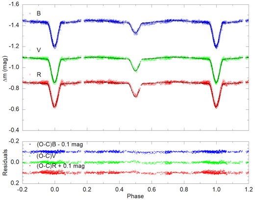
Top panel: phase-folded light curves (open circles) of HIP 7666 in B, V, and R bands and the theoretical syntheses (black solid lines) in blue, green, and red colours, respectively. Bottom panel: residuals of fits.
Basic information of the observed stars from the SIMBAD Astronomical Database.
| Stars | R.A. | Decl. | B | V | B–V |
|---|---|---|---|---|---|
| (ep = J2000) | (ep = J2000) | (mag) | (mag) | (mag) | |
| HIP 7666 | 01h38m41|${_{.}^{\rm s}}$|67 | +52°31′07|${_{.}^{\prime\prime}}$|67 | 10.04 | 9.64 | 0.4 |
| Comparison | 01h38m31|${_{.}^{\rm s}}$|76 | +52°31′58|${_{.}^{\prime\prime}}$|40 | 11.24 | 10.68 | 0.56 |
| Check 1 | 01h39m10|${_{.}^{\rm s}}$|85 | +52°34′11|${_{.}^{\prime\prime}}$|63 | 11.89 | 10.38 | 0.51 |
| Check 2 | 01h38m43|${_{.}^{\rm s}}$|14 | +52°28′28|${_{.}^{\prime\prime}}$|04 | 12.56 | 11.12 | 1.44 |
2.2 Spectroscopy
2.2.1 High-resolution spectra
High-resolution spectroscopic observations for HIP 7666 were performed using the 2.12-m telescope at the Observatorio Astronómico Nacional on the Sierra San Pedro M|$\acute{a}$|rtir (OAN-SPM) in México on November 3 and 5 of 2015. A 2048 × 2048 E2V CCD-4240 was employed to collect the echelle spectra (R = 18 000 at 5000 Å) with the slit size 1 arcsec. The spectral coverage range is from 3800 to 7100 Å. Some additional observations were made with the 2.4-m telescope on December 18 and 20 of 2016, with the fiber-fed High Resolution Spectrograph (HRS) instrument at Lijiang Station, Yunnan Astronomical Observatory (YAO) in China. The spectrograph was equipped with a 4096 × 4096 E2V CCD-203-82. The resolution was R = 32 000 corresponding to 2.0 arcsec aperture fiber. The spectral coverage range is from 3800 to 10 000 Å. A detailed journal of high-resolution spectroscopic observations is given in Table 4. A total of 10 double-line high-resolution spectra were obtained.
Journal of high-resolution spectroscopic observations for HIP 7666.
| Date | Observatory | Telescope | Instrument | Spectra |
|---|---|---|---|---|
| 2015 Nov. 3 | SPM | 2.12m | Echelle | 4 |
| 2015 Nov. 5 | SPM | 2.12m | Echelle | 2 |
| 2016 Dec. 18 | YAO | 2.4m | HRS | 2 |
| 2016 Dec. 20 | YAO | 2.4m | HRS | 2 |
| Date | Observatory | Telescope | Instrument | Spectra |
|---|---|---|---|---|
| 2015 Nov. 3 | SPM | 2.12m | Echelle | 4 |
| 2015 Nov. 5 | SPM | 2.12m | Echelle | 2 |
| 2016 Dec. 18 | YAO | 2.4m | HRS | 2 |
| 2016 Dec. 20 | YAO | 2.4m | HRS | 2 |
As far as data reduction, we first performed the preliminary spectrum-processing, involving bias and flat calibration by using the iraf/ccdred package. Then, the cosmic rays were effectively removed from the object images using the stsdas/lacos_spec package in iraf. Finally, the IRAF/ECHELLE package was used for the data reduction to obtain the normalized spectra.
2.2.2 Low-resolution spectra
Low-resolution spectroscopic observations were performed with the Yunnan Faint Object Spectrograph and Camera (YFOSC) instrument of the Lijiang 2.4-m telescope in YAO, and the Beijing Faint Object Spectrograph and Camera (BFOSC) instrument of the Xinglong 2.16-m telescope in National Astronomical Observatories of China (Fan et al. 2016), respectively. The observations were taken on December 18 and 20 of 2019 and January 10 of 2020 with the slit width of 1.5 arcsec, grating G3 on YFOSC, and the slit width of 2.3 arcsec, grating G4 on BFOSC. The spectral coverage ranges are from 3400 to 9100 Å for YFOSC, and 3600 to 8700 Å for BFOSC. The typical seeing values were 1.5 arcsec, 2.3 arcsec, and 2.4 arcsec, with the exposure time of 300 and 600 s, respectively. A detailed journal of low-resolution spectroscopic observations is given in Table 5, and a total of 7 spectra were obtained. The spectra were reduced by using standard iraf spectroscopy routines. The observations were alternated with spectra of He-Ne for YFOSC and those of Fe-Ar for BFOSC. The flux calibration of the system is performed with the standard star HR718. The results are shown in Fig. 2.
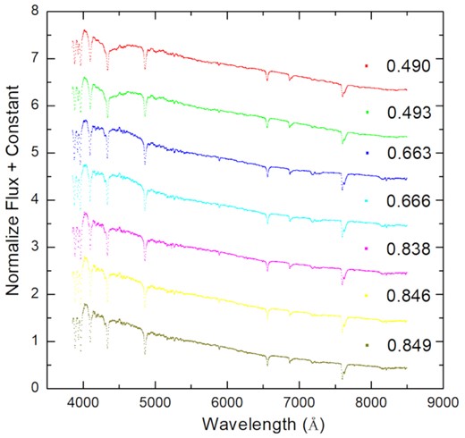
Low-resolution spectra of HIP 7666 at different phases.
Journal of low-resolution spectroscopic observations for HIP 7666.
| Date | Observatory | Telescope | Instrument | Spectra |
|---|---|---|---|---|
| 2019 Dec. 18 | YAO | 2.4m | YFOSC | 3 |
| 2019 Dec. 20 | YAO | 2.4m | YFOSC | 2 |
| 2020 Jan. 10 | NAO | 2.16m | BFOSC | 2 |
| Date | Observatory | Telescope | Instrument | Spectra |
|---|---|---|---|---|
| 2019 Dec. 18 | YAO | 2.4m | YFOSC | 3 |
| 2019 Dec. 20 | YAO | 2.4m | YFOSC | 2 |
| 2020 Jan. 10 | NAO | 2.16m | BFOSC | 2 |
3 BINARY SOLUTION
3.1 Radial velocity measurements
Radial velocities of the two components of HIP 7666.
| HJD | Phase | V1 | V2 |
|---|---|---|---|
| (2457 000+) | (km s−1) | (km s−1) | |
| 329.67574 | 0.84226 | 68.3 ± 4.4 | −117.8 ± 6.9 |
| 329.69831 | 0.85117 | 65.8 ± 4.2 | −112.0 ± 9.2 |
| 329.73418 | 0.86689 | 59.3 ± 4.0 | −104.4 ± 6.8 |
| 331.75669 | 0.87651 | 55.4 ± 2.4 | −106.3 ± 6.5 |
| 331.78604 | 0.73184 | 76.5 ± 5.8 | −138.1 ± 5.2 |
| 331.81009 | 0.74198 | 78.2 ± 7.1 | −137.9 ± 4.3 |
| 741.05343 | 0.2569 | −109.0 ± 4.5 | 108.1 ± 3.2 |
| 741.07811 | 0.2673 | −107.9 ± 3.6 | 105.0 ± 3.4 |
| 743.01943 | 0.08566 | −68.7 ± 3.8 | 53.8 ± 4.7 |
| 743.04248 | 0.09538 | −70.5 ± 4.2 | 54.4 ± 5.7 |
The RV curves are shown in the top panel of Fig. 3, with the measurements for the primary component shown as the blue open triangles and for the secondary the red open circles. The solid lines in the panel show the best fitting with velocity amplitudes of K1 = 98.6 km s−1 and K2 = 122.8 km s−1, indicating a mass ratio of q = 0.803(4), and a systemic velocity of Vγ = −15.2(7) km s−1. The bottom panel shows the residuals of the best fitting.
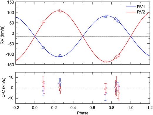
Top panel: comparison of the observed RVs of the primary (blue open triangles) and the secondary (red open circles) of HIP 7666 with the synthetic curves (solid lines). Bottom panel: residuals of fits.
3.2 Effective temperature, vsini and metallicity of the primary component
To derive effective temperature Teff,1 of HIP 7666, the PHOENIX library (Husser et al. 2013) of high-resolution synthetic spectra is used by fitting the right wing of the Hα Balmer lines that contributed most to the light by the primary. We convolve the synthetic spectra at a phase of 0.74 with a Gaussian profile having a full width at half-maximum (FWHM) = 0.36 Å to obtain the same spectrograph resolution, and adopt the surface gravity log g and metallicity [Fe/H] to be 4.0 and 0.0 dex, respectively. The Teff,1 value is searched for in the range of 6600–7400 K with the step of 200 K. Finally, considering the minimum difference of the line wing profile between the PHOENIX library spectra and observed ones, the Teff,1 value of the primary component is derived to be 7000 K. In Fig. 4, we show a comparison between model spectra from PHOENIX and HIP 7666 spectra in the region around Hα.
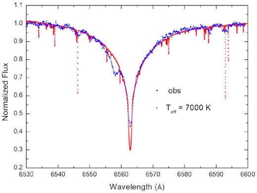
Comparison between the PHOENIX and HIP 7666 spectra in the region around Hα.
To determine the Teff,1 value of HIP 7666, we also compare the low-resolution spectra with empirical spectral templates of Kesseli et al. (2017). The spectral type of F1V is reflected at the phases 0.49 and 0.493 close to 0.5, at this phase the luminosity of the primary component dominates. At other phases of observations, the same spectral type is reflected. The result derived from low-resolution spectra is consistent with those from high-resolution spectra. Finally, we adopt the Teff,1 = 7100(100) K for the primary component.
For measuring the rotational velocity v1sini and metallicity [M/H]1 of the primary component, we apply the synthetic spectral fitting technique offered by the code iSpec (Blanco-Cuaresma et al. 2014; Blanco-Cuaresma 2019), employing the solar abundance of Grevesse & Sauval (1998), the ATLAS9 atmospheric model (3500 K ≤ Teff ≤ 50 000 K, 0.0 dex ≤ log g ≤ 5.0 dex) of Kurucz (2005), the radiative transfer code SPECTRUMof Gray & Corbally (1994), and the Vienna Atomic Line Database (VALD; Piskunov et al. 1995). For avoiding the effect from the telluric lines, we use spectra from 500 to 550 nm with high S/N for synthetic fitting. In the iteration process, the limb darkening is fixed at 0.6 (Hestroffer & Magnan 1998; Blanco-Cuaresma 2019; Sarmento et al. 2020). The micro- and macro-turbulence velocity vmic, vmac follow an empirical relation (Sheminova 2019) provided by iSpec. The effective temperature Teff, gravity log g, metallicity [M/H], rotational velocity vsini, and spectral resolution are set freely while fitting in the first run. We fix the Teff at 7100 K (see Section 3.2) and gravity log g at 3.98 (see Section 3.4) in the second run and similar results are obtained for the rest of the parameters. The part of the spectra fitting is shown in Fig. 5 for the 500–515 nm region, according to an estimation of v1sini and [M/H]1 as 41(5) km s−1 and −0.13(5) dex, respectively.
![Top panel: comparison of the fitted spectrum (red line, with Teff = 7100 K, log g = 3.98 dex, vsini = 41 km s−1, and [M/H] = −0.13 dex) and the observed spectrum of HIP 7666 (black line). Bottom panel: residuals of the fitting.](https://oup.silverchair-cdn.com/oup/backfile/Content_public/Journal/mnras/508/1/10.1093_mnras_stab2063/1/m_stab2063fig5.jpeg?Expires=1750397099&Signature=KU1-78b8E6GQgdQvVeNe34nMssiEa9okx7ooEo7k1CCpcH1LnDvvP8JlmadbCrlGEswLxFTrFJokusbZFGEjxBPNPtVCvTQsjfZpgozDPNvzJQ~SCga2O1-7jVwChcSdQDs8GFcbohqQ4PF89SOY8pfLpHJUoOISNQ2~L-E9pxW-ZslwaWa-jOkrxbLrYG~8A20J~LWdax3RkCggN3~8MrYeTPSMN9ocET9y7O1Ud64tK~xzIrHJMdWcjBCRaGOC7rClj9EmEW9O1FTbk~1I~5mTVg-27gQVL3qjqC3n1nSaysIwgGAH18-dn~sGNpDTB1PeFGw4f5sFJwqdicOFZA__&Key-Pair-Id=APKAIE5G5CRDK6RD3PGA)
Top panel: comparison of the fitted spectrum (red line, with Teff = 7100 K, log g = 3.98 dex, vsini = 41 km s−1, and [M/H] = −0.13 dex) and the observed spectrum of HIP 7666 (black line). Bottom panel: residuals of the fitting.
3.3 New ephemeris
Times of light minima of HIP 7666 and the residuals in respect to the derived ephemeris.
| HJD | Min | Epoch | O−C | Reference |
|---|---|---|---|---|
| (HJD2450000+) | d | |||
| 1769.5620 | I | −2336.0 | −0.0041 | E. Escolà-Sirisi et al.(2005) |
| 1775.4888 | II | −2333.5 | −0.0078 | E. Escolà-Sirisi et al.(2005) |
| 1775.4946 | II | −2333.5 | −0.0020 | E. Escolà-Sirisi et al.(2005) |
| 1781.4203 | I | −2331.0 | −0.0069 | E. Escolà-Sirisi et al.(2005) |
| 1782.6166 | II | −2330.5 | 0.0033 | E. Escolà-Sirisi et al.(2005) |
| 1788.5385 | I | −2328.0 | −0.0053 | E. Escolà-Sirisi et al.(2005) |
| 1845.4748 | I | −2304.0 | −0.0023 | E. Escolà-Sirisi et al.(2005) |
| 1845.4750 | I | −2304.0 | −0.0021 | E. Escolà-Sirisi et al.(2005) |
| 7311.0711 | I | 0.0 | −0.0009 | this work |
| 7311.0726 | I | 0.0 | 0.0006 | this work |
| 7311.0719 | I | 0.0 | −0.0001 | this work |
| 7313.4458 | I | 1.0 | 0.0016 | this work |
| 7313.4450 | I | 1.0 | 0.0008 | this work |
| 7313.4457 | I | 1.0 | 0.0015 | this work |
| 7318.1881 | I | 3.0 | −0.0006 | this work |
| 7318.1879 | I | 3.0 | −0.0008 | this work |
| 7318.1876 | I | 3.0 | −0.0011 | this work |
| 7353.7725 | I | 18.0 | 0.0005 | this work |
| 7353.7728 | I | 18.0 | 0.0008 | this work |
| 7353.7721 | I | 18.0 | 0.0001 | this work |
| 7356.1446 | I | 19.0 | 0.0004 | this work |
| 7356.1444 | I | 19.0 | 0.0002 | this work |
| 7356.1441 | I | 19.0 | −0.0001 | this work |
| 7394.0990 | I | 35.0 | −0.0007 | this work |
| 7394.0981 | I | 35.0 | −0.0016 | this work |
| 7394.0988 | I | 35.0 | −0.0009 | this work |
3.4 Photometric solution
By using the newly derived linear ephemeris, all the measurements are transferred into phases, as shown in the top panel of Fig. 1. The general features of the light curves show typical Algol-type EBs with nearly total eclipses, suggesting a large inclination close to 90°. The magnitude variations are measured to be about 0.246, 0.235, and 0.233 mag for the primary eclipse and about 0.117, 0.12, and 0.127 mag for the secondary eclipse in B, V, and R bands, respectively.
A photometric solution of the binary system is searched for in order to derive the system parameters with the complete light curves in B, V, and R bands and the RV curves of the primary and second components. The 2013 version of Wilson–Devinney code (Wilson & Devinney 1971; Wilson 1979, 1990) is used for the numerical light-curve analysis. The non-linear limb-darkening law with a logarithmic form is applied in the analysis progress. We get the parameter of parallax of this star to be 3.1732 ± 0.0389 millisecond of arc from DR2 of the Gaia catalogue. The temperature of primary component T1 is fixed at 7100 K (see Section 3.2), while the temperature of the second one T2 is adjustable. Considering the evolutionary status of classical Algol-type EBs, we set the eccentricity e = 0, the argument of periastron ω0 = 0, and synchronous rotation F1 = F2 = 1. The values of bolometric albedos A1 and A2 and gravity-darkening coefficients g1 and g2 are assumed as A1 = 1 and g1 = 1 for radiative (von Zeipel 1924; Ruciński 1969) and A2 = 0.5 and g2 = 0.32 for convective atmospheres (Lucy 1967). The initial bolometric (X1, X2, Y1, Y2) and monochromatic (x1, x2, y1, y2) limb-darkening coefficients of the components are taken from the tables of van Hamme (1993).
According to the preliminary photometric solution published by Escolà-Sirisi et al. (2005), HIP 7666 is a detached configuration system (mode 2). A semidetached solution is also tested, but the result is worse than that of the detached configuration. First, we search for a solution to the orbital model by changing the mass ratio q = m2/m1, semimajor axis a, and RV Vγ of the centre of mass of the system. Then, fixing the derived values q = 0.803, a = 10.48 R⊙, and Vγ = −15.2 km s−1, we search for a solution that fits the light and RV curves the best by changing the effective temperature of the second component T2, orbital inclination i, dimensionless bandpass luminosity of primary L1, and surface potentials Ω1 and Ω2. Later on, the final solution for the detached binary HIP 7666 is shown in the top panel of Fig. 1 with black solid lines, and the residuals of O − C are plotted in the bottom panel of Fig. 1 including the pulsations periodic patterns.
The final solutions of HIP 7666 are listed in Table 8. Besides the parameters derived from phase-folded light and radial-velocity curves directly, the masses (M), radii (R), absolute magnitudes (Mbol), and surface gravities (log g) are also calculated. According to the radius and effective temperature, we can obtain the luminosity of the system [L = 11.1(7) L⊙], which is consistent with the luminosity obtained by Gaia (LGaia = 11.12 L⊙). All these parameters are also listed in Table 8.
Parameters of HIP 7666 from W–D fits of light and radial-velocity curves.
| Parameter | Primary | Secondary | |
|---|---|---|---|
| ea | 0.0 | ||
| Fa | 1.0 | 1.0 | |
| ga | 1.0 | 0.32 | |
| Aa | 1.0 | 0.5 | |
| (X, Y)a | 0.638, 0.256 | 0.645, 0.221 | |
| (xB, yB)a | 0.787, 0.284 | 0.827, 0.187 | |
| (xV, yV)a | 0.687, 0.292 | 0.743, 0.259 | |
| (xR, yR)a | 0.588, 0.294 | 0.650, 0.269 | |
| i(deg) | 81.85(3) | ||
| Teff(K) | 7100(100)b | 6029(67) | |
| Ω | 5.87(1) | 9.04(4) | |
| |$\Omega _{\mathrm{ in}}\, ^a$| | 3.42 | ||
| |$\Omega _{\mathrm{ out}}\, ^a$| | 2.97 | ||
| q = M2/M1 | 0.803(4) | ||
| L1/(L1 + L2)B | 0.9087(1) | ||
| L1/(L1 + L2)V | 0.8870(1) | ||
| L1/(L1 + L2)R | 0.8714(2) | ||
| rpole | 0.197(1) | 0.101(1) | |
| rpoint | 0.201(1) | 0.102(1) | |
| rside | 0.198(1) | 0.102(1) | |
| rback | 0.200(1) | 0.102(1) | |
| Porb(d) | 2.372 2200(4) | ||
| a(R⊙) | 10.48(7) | ||
| Vγ(km s−1) | −15.2(7) | ||
| M(M⊙) | 1.53(3) | 1.23(3) | |
| R(R⊙) | 2.08(2) | 1.06(2) | |
| log(L/L⊙) | 0.99(3) | 0.13(4) | |
| log g | 3.98(2) | 4.47(2) | |
| Mbol | 2.26(8) | 4.4(1) |
aAssumed, bresult from spectroscopy.
3.5 Age and evolutionary status
The filling factors [|$\it {f} = \left(\Omega _{\mathrm{ in}} - \Omega \right)/\left(\Omega _{\mathrm{ in}} - \Omega _{\mathrm{ out}}\right)$|] of both components, which are derived from the results of the photometric solutions as listed in Table 8, are less than zero. This indicates that HIP 7666 is a detached EB system and has no material exchange during the stellar evolution between the stars.
To derive the age of the investigated system, we compare the observed properties of the stars, i.e. effective temperature, luminosity with a web interface the PAdova and TRieste Stellar Evolution Code1 (parsec, version 1.2S; Bressan et al. 2012) isochrones. An estimated metallicity derived from spectra fitting is adopted in this work, and we assume that the secondary component has the same metallicity as the primary ([M/H] = −0.13 dex). The relationship of solar-scaled composition follows Y = 0.2485 + 1.78Z, and the present solar metal content is Z⊙ = 0.0152. In Fig. 6, three isochrones of age = 1.45, 1.69, and 1.95 Gyr are plotted in both the Teff − log(L/L⊙) (H–R) and Teff − log g diagrams with the dashed, solid, and dotted lines, respectively. The locations of primary and secondary components marked with blue and red pentagram symbols are fitted within the ±3σ credible region. In the H–R diagram, the estimated age of the system is |$1.69_{-0.24}^{+0.26}$| Gyr based on the confidence interval for the effective temperature of the primary component. Similarly, good fits are shown in the top panel of the figure.
![PARSEC isochrones for HIP 7666 and [M/H] = −0.13 dex. Dashed, solid, and dotted lines are isochrones for age = 1.45, 1.69, and 1.95 Gyr, respectively. The locations of the primary and secondary components are marked with blue and red pentagram symbols, both with ±3σ error bars.](https://oup.silverchair-cdn.com/oup/backfile/Content_public/Journal/mnras/508/1/10.1093_mnras_stab2063/1/m_stab2063fig6.jpeg?Expires=1750397099&Signature=Pw0OQVejBv8Igmt7ekCBQZwmXJWtI12t1kmClC4UALso5rN1mYGnalMws~unXnrsstkJbNOCH4c5aqdCwiG6HUhX6PHUqenvaFx6kNx0Y8maPoenCVMaAAzW8HaaH7rmx1pxhqp56xn8Y4rhNmJd~nu-75otsKbbo5Iu~gOjl30eEHDefJ8GnkAFLjfHH-NCRBNvolVWNVoJijyOrQ3FcVq5UnIFlhU~A0qQ8pu4oboJZ5Sb8k20hjR1o6cM5aWXJ8CoD88AiPBwjF1MlGwm47onlDbTPMfO4XjlCXPyqbfDLmN~5vcJOG7~JRNtGQLv0rRKwWrl9-b0dUuopdAJBQ__&Key-Pair-Id=APKAIE5G5CRDK6RD3PGA)
PARSEC isochrones for HIP 7666 and [M/H] = −0.13 dex. Dashed, solid, and dotted lines are isochrones for age = 1.45, 1.69, and 1.95 Gyr, respectively. The locations of the primary and secondary components are marked with blue and red pentagram symbols, both with ±3σ error bars.
Since HIP 7666 is a detached EB system that has no mass transfer between the stars, the single-star evolutionary models computed with mesa (Modules for Experiments in Stellar Astrophysics, version 9793; Paxton et al. 2011, 2013, 2015) are used to estimate the evolutionary status of the stars. All models are calculated with the OPAL equation-of-state tables (Rogers & Nayfonov 2002). The OPAL opacity tables (Iglesias & Rogers 1996) are used for the high temperatures and the tables of Ferguson et al. (2005) for the low temperatures. We adopt gs98 (Grevesse & Sauval 1998) solar heavy element distribution and use ‘simple_photosphere’ for the atmosphere boundary condition. The initial hydrogen and helium abundances are set to Z = 0.0123 and Y = 0.2654, respectively, based on the metallicity [M/H] = −0.13 dex from the iSpec analysis and the linear relation Y = 0.249 + 1.33Z (Li et al. 2018). In the convective region, the classical mixing-length theory of Böhm-Vitense (1958) is used. The mixing-length parameters αMLT of the primary and secondary components are calculated to be 2.4 and 2.2 by using the equation (2.1) provided by Yıldız (2008), respectively. Fig. 7 is the H–R diagram for stellar evolutionary models with M = 1.53 M⊙ (blue line) and M = 1.23 M⊙ (red line). The locations of the primary and secondary components are marked with blue and red pentagram symbols, respectively, with the ±3σ error bars. It can be seen that the primary component is in good agreement with the theoretical model but the secondary, although within the ±3σ error bars, deviates somewhat from its evolutionary track. Similar discrepancies have been observed in other EBs by Clausen et al. (2010), Torres et al. (2014), and Matson et al. (2016). They suggest that this difference between models and observations is maybe due to a complex relationship between overshooting, mass, and metallicity. Four evolutionary stages of the primary components are labelled as A = 1.45 Gyr, B = 1.55 Gyr, C = 1.65 Gyr, and D = 1.755 Gyr, respectively. The age of the evolution stage D, on which the effective temperature and luminosity of the primary component are almost exactly matched, is consistent with the age given by parsec isochrones. As shown in Fig. 7, the primary component has evolved to the late stages of the main sequence, while the secondary still locates at the early stages of the main sequence.
![mesa evolutionary tracks computed for the primary (M = 1.53 M⊙, [M/H] = −0.13 dex, blue line) and secondary (M = 1.23 M⊙, [M/H] = −0.13 dex, red line) components of HIP 7666 in H–R diagram. Blue and red pentagram symbols represent the primary and secondary components, respectively, with their ±3σ error bars. Four evolutionary stages for primary component are labelled as A, B, C, and D.](https://oup.silverchair-cdn.com/oup/backfile/Content_public/Journal/mnras/508/1/10.1093_mnras_stab2063/1/m_stab2063fig7.jpeg?Expires=1750397099&Signature=sySEnzousR-lpGvVJE3UjuwAJiUtVSMMtRpMUEXo7DvQ7RVdPIfMVBI0jljNxF377iDRIgT2A6UN-QhEC7GCkt6vp8-DXZnx0xKQt0W5reKrvgF4~y14o42sjCJViMONG2c9m2n-ERUpfAY8ykJ03tHjZmDAVlE-3qVn3NHp~vNVRE33PYChT9p7nNXg9p7GWqwkQ8S0b6EBA9n0E9d~7JDCHVnrAwvsegrBF7mv4ovrLkSIIydClt-2E7inzNmT9MK8LT-dhuOoVaHBI~5lv9gr-9EzH1EvlS-XXjQ16ZpQb-QYqkib2LunSHDbj6fblQQBSNt8osG6LSqhN3wnaQ__&Key-Pair-Id=APKAIE5G5CRDK6RD3PGA)
mesa evolutionary tracks computed for the primary (M = 1.53 M⊙, [M/H] = −0.13 dex, blue line) and secondary (M = 1.23 M⊙, [M/H] = −0.13 dex, red line) components of HIP 7666 in H–R diagram. Blue and red pentagram symbols represent the primary and secondary components, respectively, with their ±3σ error bars. Four evolutionary stages for primary component are labelled as A, B, C, and D.
4 PULSATION ANALYSIS
4.1 Fourier analysis of the residual light curve
In order to analyse the pulsating nature of the binary system in detail, we extract the pulsational light variations only containing oscillation information from the original observation data with the method of Zhang, Zhang & Li (2009). To prepare for frequency analysis, the photometric solution is subtracted, and second or third-order polynomials are used to fit the light curves to eliminate the low-frequency effects caused by the long-term instability of atmospheric transparency and instrumentation (Chen et al. 2019). Considering that the amplitudes of the pulsation are of the order of milli-magnitude, only the data with photometric precision higher than 0.01 mag are used.
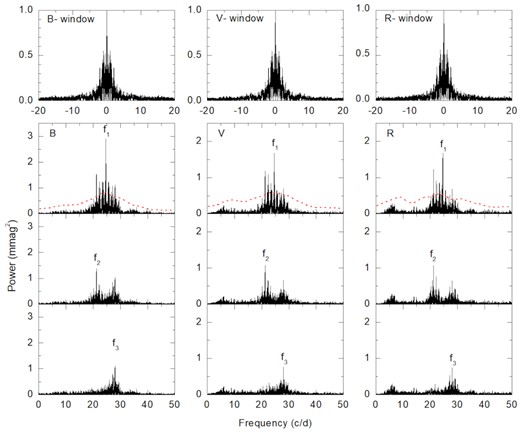
Fourier power spectra of the light residuals for HIP 7666 in B, V, and R bands. The upper panels show the window spectra. The dashed lines in red present the 4σ noise level.
Results of the frequency analysis.
| ID | Filter | Frequency | Amplitude | S/N |
|---|---|---|---|---|
| (cd−1) | (mmag) | |||
| B | 24.631(4) | 1.6(1) | 7.0 | |
| f1 | V | 24.64(2) | 1.2(1) | 6.7 |
| R | 24.61(2) | 1.1(1) | 7.4 | |
| B | 21.193(1) | 1.3(1) | 5.2 | |
| f2 | V | 21.191(8) | 1.0(1) | 5.3 |
| R | 21.194(1) | 1.1(1) | 4.8 | |
| B | 28.07(7) | 0.9(3) | 4.5 | |
| f3 | V | 28.1(1) | 0.8(1) | 5.0 |
| R | 28.10(8) | 0.6(2) | 5.1 |
Compared the physical parameters of the components in Table 8 with the typical mass, effective temperature, luminosity, and period range of δ Scuti type variables (Breger 2000), the primary component of HIP 7666 fits better to the profile of δ Scuti stars.
4.2 Asteroseismic models
Only three frequencies are detected in this work, it is difficult to constrain the stellar models. We present an asteroseismic interpretation of radial oscillations (l = 0) and non-radial oscillations (l = 1, 2) modes using the submodule ‘pulse_adipls’ of mesa for the primary component of HIP 7666, as the amplitudes of disc-integrated photometry are hardly to be observed for oscillation modes with l > 2. The input physics is the same as the single-star evolution model (see Section 3.5). Other parameters, initial_mass, initial_Z, and initial_Y, are fixed to 1.53, 0.0123, and 0.2654, respectively. The effects of the stellar rotation, the convective overshooting, and magnetic fields on the evolution models are not considered.
We investigate nine evolutionary stages from the age of 1.45 Gyr to 1.8 Gyr, with an interval of 0.05 Gyr. In Fig. 9, only the results of four evolution stages of A = 1.45 Gyr, B = 1.55 Gyr, C = 1.65 Gyr, and D = 1.755 Gyr are shown. The top panel is for l = 2 modes, the middle panel for l = 1 modes, and the bottom panel for l = 0 modes. The dashed lines present f1 = 24.631 cd−1, f2 = 21.193 cd−1, and f3 = 28.07 cd−1, respectively. Radial orders from 1 to 5 are represented by circles of different colours. It can be seen that the theoretical frequencies of models A and C cannot match the observed ones well. On stage B, we tentatively identify the most possible pulsation modes as (l, n) = (0, 4) or (2, 2) for f1, (0, 3) or (2, 1) for f2, and (0, 5) or (2, 3) for f3. On stage D, the most possible pulsation modes are (l, n) = (1, 3) for f1, (1, 2) for f2, and (1, 4) for f3.
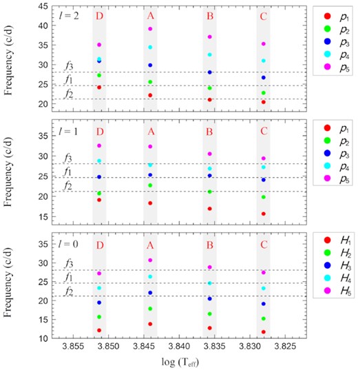
The theoretical pulsation frequencies for primary component of HIP 7666 calculated with MESA corresponding to the four evolutionary stages A, B, C, and D (the same as Fig. 7). The top panel is for l = 2 modes, the middle panel for l = 1 modes, and the bottom panel for l = 0 modes. Radial orders from 1 to 5 are represented by circles of different colours. The dashed lines present the observed frequencies f1 = 24.631 cd−1, f2 = 21.193 cd−1, and f3 = 28.07 cd−1, respectively.
4.3 Large frequency spacing
For HIP 7666, the frequency difference between f1 and f2 (3.438 cd−1) is nearly equal to that between f1 and f3 (3.439 cd−1). Considering that the harmonics of the orbital frequency are a possible cause of such equally spaced frequencies, we search for possible frequency combinations with the orbital frequency Forb = 0.421546 cd−1 and find that f1, f2, and f3 are not combinations of the orbital harmonics. Previous studies on the δ Scuti stars have found such large equally spaced frequencies, and suggested that this may be related to the eigenfrequencies or the rotation splitting frequencies (Kim et al. 2010; García Hernández et al. 2013; Ou, Yang & Zhou 2019).
However, using equation (7), the rotation period of the primary component of HIP 7666 is calculated to be approximately 0.58 d and the equatorial velocity of vrots ≈ 182 km s−1, which is seriously inconsistent with the result (41 km s−1) from spectral fitting, is obtained according to the primary’s radius (R = 2.08 R⊙). On the other hand, Zahn (1975) recommended that tidal braking is most significant when the orbital period is less than 10 d. Lurie et al. (2017) inspected 816 EBs with star-spot modulations from the Kepler Eclipsing Binary Catalog, and find that 79 per cent of them with orbital periods of less than 10 d are synchronized, and EBs with orbital periods of less than 2 d are nearly all synchronized. For synchronous rotation, the rotation period of the primary component is approximately equal to the orbital period of 2.37 222 d, and the rotational velocity is approximately 43 km s−1. This is very consistent with the result of iSpec analysis.
Although the amplitude of f3 is almost the same as the amplitude of f1 and f2, the possibility that f3 is a combination of f1 and f2 (f3 = 2f1 – f2) cannot be ruled out completely.
4.4 Discussion of pulsation modes
HIP 7666 is a detached binary system with an orbital period of 2.372 2200(4) d. The primary component of this system is a δ Scuti star. A total of three significant frequencies [f1 = 24.631(4) cd−1, f2 = 21.193(1) cd−1, and f3 = 28.07(7) cd−1] are extracted. In this subsection, we will give a brief discussion on the pulsation modes of the three frequencies.
The frequency (or the pulsation constant Q) variation of each radial order remains nearly constant for radial pulsations (l = 0) with evolution (Osaki 1975). That means different radial orders have different pulsation constants. But in our study, the radial orders [n = 4 (f1), n = 3 (f2), and n = 5 (f3)] derived from the model B of the primary component of HIP 7666 are different from the values ([n = 3 (f1), n = 2 (f2), and n = 4 (f3)] based on the pulsation constant Q from Fitch (1981). On the other side, the frequencies (f1, f2, and f3) have period ratios of P1/P2 = 0.86 and P3/P1 = 0.877, which are far away from the expected values of the radial modes (Stellingwerf 1979; McNamara 2011). Moreover, the radial modes always possess high amplitudes (Pych et al. 2001; Olech et al. 2005; Yang et al. 2018), but the three frequencies in this work have very low amplitudes, ΔV ∼ 1 mmag. Therefore, it seems that these three frequencies are unlikely radial modes.
In the case of l = 2 mode, the radial orders are n = 2 for f1, n = 1 for f2, and n = 3 for f3 derived from model B of the primary component of HIP 7666. However, following the paper by Fitch (1981), the values of Q1, Q2, and Q3 are quite different from the values of second, first, and third radial orders. For l = 1 mode, the corresponding radial orders are n = 3 for f1, n = 2 for f2, and n = 4 for f3 on evolution stage D, on which the physical parameters, such as effective temperature and luminosity of the primary component are almost exactly matched with the theoretical models. However, by comparing with models of Fitch (1981), we find that the values of Q1, Q2, and Q3 are slightly smaller than the theoretical ones. Since the primary component is in an evolved state, the pulsation constant Q will change step-wise for non-radial modes with evolution (Osaki 1975). This may be the reason of the lower Q values.
5 SUMMARY AND DISCUSSION
In this paper, detailed photometric and spectroscopic analysis of HIP 7666 are presented. First, we carried out a new multisite and multicolour photometric observations for this binary during 22 nights, and obtained multicolour light curves with complete phase coverage. A total of six primary eclipses including 18 light minima in three bands are covered. Combining with the other eight light minima observed by Escolà-Sirisi et al. (2005), a new linear ephemeris is given by utilizing the least-square fitting. Secondly, high-resolution spectroscopic observations were carried out synchronously on four nights with a total of 10 double-line spectra obtained. RVs of the primary and secondary components are analysed and the results are improved together with the light curves. Finally, the effective temperature Teff,1 of the primary component is determined to be 7100(100) K by both high- and low-resolution spectra, and the rotational velocity v1sini and metallicity [M/H] are estimated to be 41(5) km s−1 and −0.13(5) dex, respectively, by the synthetic spectral fitting method with iSpec.
By using the light and RV curves of HIP 7666, we obtain orbital solutions of the system with the W–D method. Using the results of LCs, the absolute astrophysical parameters are calculated. Our results show that HIP 7666 is a detached binary system with the absolute parameters M1 = 1.53(3) M⊙, R1 = 2.08(2) R⊙, log L1/L⊙ = 0.99(3), log g1 = 3.98(2), Mbol1 = 2.26(8), Teff,1 = 7100(100) K for the primary, and M2 = 1.23(3) M⊙, R2 = 1.06(2) R⊙, log L2/L⊙ = 0.13(4), log g2 = 4.47(2), Mbol2 = 4.4(1), Teff,2 = 6029(67) K for the secondary. Then, the estimated age of 1.69 Gyr and 1.755 Gyr are derived by comparing the absolute parameters with PARSEC isochrones and MESA evolutionary tracks. In H–R diagram, the primary component has evolved to the late stages of the main sequence, while the secondary still locates at the early stages of the main sequence. Since the number of δ Scuti stars located in confirmed detached binaries is very small, especially for double-line spectroscopic binaries whose absolute parameters could be calculated with RV and light curves (Liakos 2017), this star could be an important one in understanding pulsating EBs.
After subtracting the photometric solution from the light curves of HIP 7666, three frequencies, f1 = 24.631(4) cd−1, f2 = 21.193(1) cd−1, and f3 = 28.07(7) cd−1, are resolved in all filters with S/N > 4. According to the absolute parameters of components and pulsating frequencies range, the primary component of HIP 7666 is a δ Scuti star located close to the terminal-age main-sequence and the red edge of δ Scuti instability strip in the H–R diagram. On account of the interaction between convection and pulsation (Dupret et al. 2004) in this region, it is difficult to determine precisely the theoretical red edge of the δ Scuti instability strip. More samples in this region will be helpful to determine the red edge.
The three frequencies yielded from the observations of HIP 7666 show the regular large spacing by 3.44(4) cd−1. Our result shows that f3 may be an eigenfrequency or possibly a combination of f1 and f2. The radial (l = 0) and non-radial (l = 1, 2) asteroseismic models of nine different evolutionary stages are constructed to fit the observed frequencies. We explored different possibilities of modes by comparing the Q values from Fitch (1981). The photometric observations from space missions are needed for reliable mode identifications, and a sequence of more detailed theoretical models with different combinations of parameters are necessary.
ACKNOWLEDGEMENTS
This paper benefited from many thoughtful comments made by the anonymous referee. We acknowledge the support from the National Natural Science Foundation of China (NSFC) through grants 11833002,11673003,11873081,U2031209, and11803076. This research is supported by the Nanshan One-meter Wide-field Telescope (NOWT) at the Nanshan Station of Xinjiang Astronomical Observatory, Chinese Academy of Sciences. We acknowledge the support of the staff of the Xinglong 2.16-m and 85-cm telescopes. This work was partially supported by the Open Project Program of the Key Laboratory of Optical Astronomy, National Astronomical Observatories, Chinese Academy of Sciences. This work was also based on the observations carried out at the Observatorio Astronómico Nacional on the Sierra San Pedro M|$\acute{a}$|rtir (OAN-SPM), Baja California’ México. We thank Raul Michel for his help in applying for the observation time of the 2.12-m and 84-cm telescopes at SPM. We acknowledge the support of the staff of the YNAO 2.4-m telescope. Funding for the telescope has been provided by the Chinese Academy of Sciences and the People′s Government of Yunnan Province. This work has made use of data from the European Space Agency (ESA) mission Gaia (https://www.cosmos.esa.int/gaia), processed by the Gaia Data Processing and Analysis Consortium (DPAC, https://www.cosmos.esa.int/web/gaia/dpac/consortium).
DATA AVAILABILITY
The data underlying this article will be shared on reasonable request to the corresponding author.
