


ABSTRACT
Very little work has been done on star formation in dwarf lenticular galaxies (S0s). We present 2D spectroscopic and millimetre observations made by the Centro Astronómico Hispano Alemán (CAHA) 3.5-m optical and Institut de Radioastronomie Millimétrique (IRAM) 30-m millimetre telescopes, respectively, for a sample of four dwarf S0 galaxies with multiple star formation regions in the field environment. We find that, although most of the sources deviate from the star-forming main-sequence relation, they all follow the Kennicutt–Schmidt law. After comparing the stellar and Hα kinematics, we find that the velocity fields of both stars and ionized gas show no regular motion and the velocity dispersions of both stars and ionized gas are low in regions with high star formation, suggesting that these star-forming S0 galaxies still have significant rotation. This view can be supported by the result that most of these dwarf S0 galaxies are classified as fast rotators. The ratio of the average atomic gas mass to stellar mass (|$\sim 47{{\ \rm per\ cent}}$|) is much greater than that of the molecular gas mass to stellar mass (|$\sim 1{{\ \rm per\ cent}}$|). In addition, gas-phase metallicities in star-forming regions are lower than those of non-star-forming regions. These results indicate that extended star formation may originate from the combination of abundant atomic hydrogen, a long dynamic time-scale, and a low-density environment.
1 INTRODUCTION
Lenticular galaxies (S0s) are introduced as a distinct morphological type in the Hubble tuning-fork diagram (Hubble 1936). They are classified as early-type galaxies (ETGs), a class of galaxies that have evolved passively after a big burst of star formation, and considered as an intermediate population between spirals and ellipticals. One of the most popular theories, hierarchical two-phase accumulation, is usually used to explain the star formation history of ETGs (Oser et al. 2010). The first phase is the main mechanism for stellar growth via gas collapse at high redshift, while the second stage is size growth by the accretion of satellite systems at low redshift. Although this scenario can successfully explain the formation of many elliptical galaxies, the formation of S0 galaxies is not yet well understood.
Previous studies have found that there are many processes that can be introduced to explain the formation of S0 galaxies. One of them is the removal of cold gas from spiral galaxies via either secular evolution or environmental effects (Moore et al. 1996; Moore, Lake & Katz 1998; Bekki 1998; Governato et al. 2009; Bekki & Couch 2011). This mechanism is responsible for the properties of low star formation and prominent bulges in S0 galaxies. On the other hand, the results from numerical simulations have shown that the merger mechanism can also produce S0-like remnants (Tapia et al. 2014; Querejeta et al. 2015). Graham, Dullo & Savorgnan (2015) suggested that compact spheroidal objects at high redshift can evolve into S0 galaxies through cold gas accretion. This accretion process at high redshift can increase the number of S0 galaxies seen in the present Universe. A recent study shows that violent disc instability could also be an important formation mechanism of S0 galaxies (Saha & Cortesi 2018).
The conventional perception is that the star formation rate (SFR) in S0 galaxies is low, which may be explained by two scenarios. The first is that S0 galaxies have little or no gas content. As found by Bregman, Hogg & Roberts (1992), most S0 galaxies have lower M(H i)/LB than spiral galaxies. The second explanation for the low SFR is morphological quenching, which is usually attributed to large and red bulges in the centres of S0 galaxies (Martig et al. 2009; Xiao et al. 2018).
However, many studies have shown that atomic and even molecular gas content is present in volume-limited samples of S0 and/or elliptical galaxies (Welch & Sage 2003; Sage & Welch 2006; Welch, Sage & Young 2010). S0 galaxies could be rather rich in neutral hydrogen, based on observations of the 21-cm line (van Driel & van Woerden 1991). Kannappan, Guie & Baker (2009) found that ETGs with star formation reside in similar regions to spirals in colour versus stellar mass space, and the fraction of ETGs with star formation increases with decreasing stellar mass. The variation in the fraction of ETGs with star formation indicates that the origins of star formation activity in ETGs might be different in different stellar mass ranges. High-mass star-forming S0 galaxies are often triggered by mergers, while low-mass S0 galaxies form stars by gas accretion.
The kinematics of ETGs are closely related to the gas content. Davis et al. (2016, 2019) presented cold gas observations of massive ETGs. They found that slow rotators or galaxies with higher velocity dispersion hold less gas. They attributed it to gas-rich merger events, but stellar mass-loss and hot halo cooling also play an important role. Similar results have been found by Young et al. (2011), who explored the relationship between the star formation history and the gas mass in ETGs using the ATLAS3D survey. They concluded that the smaller the angular momentum of ETGs, the lower the gas content, suggesting that formation processes for slow rotators can effectively destroy molecular gas or prevent gas from accreting. However, Serra et al. (2012, 2014) found that a large diversity of |${\rm H\, \small {I}}$| masses and morphologies, not only within fast rotators but also within slow rotators and neutral hydrogen, can provide fresh gas for residual star formation in ETGs. A recent study also found that the external accretion of gas may fuel star formation or an active galactic nucleus (AGN: Raimundo 2021).
Xiao et al. (2016) studied nuclear activity in nearby S0 galaxies using Sloan Digital Sky Survey Data Release 7 (SDSS DR7) and found that roughly 8 per cent of S0 galaxies show central star formation activity. It should be noted that this fraction might be higher, considering that low-level star formation, which is often present in objects with low-ionization nuclear emission-line regions, may be missed if it is only investigated through optical spectral analysis. Therefore, the number of star-forming S0 galaxies in Xiao et al. (2016) should be considered a lower limit. In order to understand the spatially resolved properties of star-forming S0 galaxies from Xiao et al. (2016), we have started a programme to obtain Integral Field Spectroscopy (IFS) data with the Centro Astronómico Hispano Alemán (CAHA) 3.5-m telescope. Based on the star-forming S0 galaxy sample, here we present four low-mass cases with multiple nuclear structures. Fig. 1 shows their false-colour (g-, r-, and i-band) images from SDSS. We note that these S0 galaxies have stellar masses |$M_{\ast }\lesssim 10^{9}\, \mathrm{M}_{\odot }$|. In order to investigate the molecular gas content in the four S0 galaxies, we simultaneously observed CO(J = 1–0) and CO(J = 2–1) with the IRAM 30-m telescope. ETGs generally have large stellar masses. Many previous studies also involved high-mass (|$\rm \log \ M_{\ast }\gt 10.0$|) samples, and few studies focus on such low-mass star-forming S0 galaxies. In this work, we hope that the combination of IFS and millimetre observations of dwarf S0 galaxies can provide important clues to the star formation history of ETGs.
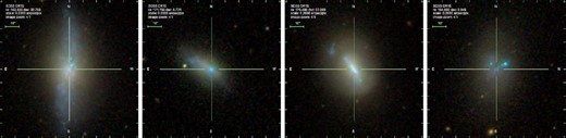
SDSS composite colour images for the four S0 galaxies. From left to right, they are PGC 32543, PGC 35225, PGC 36686, and PGC 44685, respectively.
This work is organized as follows. In Section 2, we show the observations and reduction of optical IFS and millimetre data. Sections 3 and 4 present the results and discussion. Finally, we give a summary in Section 5. We assume constant cosmographic parameters where ΩM = 0.3, ΩΛ = 0.7, and H = 70 km s−1 Mpc−1 and adopt a Salpeter (1955) initial mass function (IMF).
2 OBSERVATIONS AND DATA REDUCTION
2.1 CAHA 2D spectroscopic observations
The sources studied in this work have been covered by spatially resolved IFS observations using the Potsdam Multi-Aperture Spectrophotometer (PMAS)/PMAS fiber PAcK (PPAK) configuration mounted on the CAHA 3.5-m telescope at the Calar Alto observatory. The multi-aperture spectrometer equipped on the telescope has 382 fibres, each with a diameter of 2.7 arcsec, which produces a hexagonal field of view (FoV) of 78 × 73 arcsec2 for our sample. The FoV is sufficient to cover entire galaxies up to two to three effective radii. CAHA observes the galaxies in two configurations (i.e. the V500 setup and the V1200 setup). The V500 setup covers wavelengths between 3745 and 7500 Å, which provides a low spectral resolution (R ∼ 850). The other setup covers the wavelength range from 3400–4840 Å, which provides a medium spectral resolution (R ∼ 1650). The objects were observed by using a three-pointing dithering scheme to obtain a filling factor of 100 per cent. The exposure time per pointing was 900 s. We used an upgraded python-based pipeline (García-Benito et al. 2015; Sánchez et al. 2016) to reduce the PPAK data. The reduction process is summarized as follows: (i) identification of the position of the spectra on the detector along the dispersion axis; (ii) extraction of an individual spectrum; (iii) distortion correction of the extracted spectrum; (iv) wavelength calibration; (v) fibre-to-fibre transmission correction; (vi) flux calibration; (vii) subtraction of the sky; (viii) data-cube reconstruction; and finally (ix) differential atmospheric correction. We recommend readers refer to Husemann et al. (2013), García-Benito et al. (2015), and Sánchez et al. (2016) for more details of the reduction process. For the original data cubes, we correct the flux for Galactic extinction. The final spectra cover fully the wavelength range from 3700–7300 Å.
2.2 Spectroscopic fitting and parameter calculation
Firstly, we use a full spectrum fitting method, Penalized Pixel-Fitting (pPXF) (Cappellari & Emsellem 2004; Cappellari 2017), to model the stellar continuum. pPXF adopts Medium-resolution Isaac Newton Telescope library of empirical spectra (MILES) simple stellar population templates (Vazdekis et al. 2010), which assume a Salpeter (1955) IMF and Calzetti et al. (2000) dust extinction curve. The template library comprises 150 templates covering 25 population ages (from 0.06–15.85 Gyr) and six metallicities (i.e. log[M/H] = −1.71, −1.31, −0.71, −0.4, 0.0, 0.22). Stellar population fitting is applied to the V500 spectra and the emission lines are masked when modelling the stellar continuum. It is noted that we do not contain an AGN in the templates, considering that these S0 galaxies were not identified as AGNs through the Baldwin, Phillips & Telervich (BPT) diagram in Xiao et al. (2016).
Next, we subtract the stellar continuum from the original spectra to obtain the ionized gas emission lines. For the emission lines, we fit them spaxel by spaxel using single Gaussian models and the width of the Gaussian was tied for ions of the same element.
Considering that the emission lines may be contaminated by AGNs or shocks, we tested the ionization mechanism of the emission lines of these galaxies. Fig. 2 shows the spatial distribution of the ionization mechanism of spaxels according to the traditional BPT diagnostic diagram (Kewley et al. 2001) and the equivalent width of Hα (Lacerda et al. 2018). We find that almost all emission lines are ionized by star formation (blue points in Fig. 2), especially in the central regions of galaxies (i.e. star formation regions). Therefore, we ignore the effects from AGNs and shocks in the calculation of the SFR.
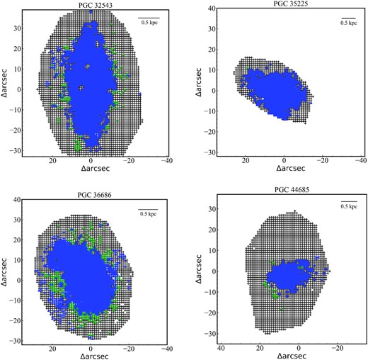
Spatial distribution of the ionization mechanism. Star formation and composite regions are marked as blue and green, respectively. The physical scale corresponding to each arcsec is marked in the upper right corner of each panel.
In order to obtain the surface mass density of atomic gas (ΣHI), we adopt a method based on gas-phase metallicity to estimate ΣHI (see Table 1). The gas-phase metallicities of the four S0 galaxies are derived based on a Bayesian method1 (Blanc et al. 2015), which assumes the Levesque, Kewley & Larson (2010) photoionization model. This method makes the probability density functions of gas-phase metallicity and ionization available after inputting a set of strong nebular emission lines. We use the stacked spectra that are used to estimate the total SFR to compute the gas-phase metallicity; this, in turn, is used to derive ΣHI according to the empirical formula of Schruba, Bialy & Sternberg (2018). We also compute the spatially resolved metallicity using a set of strong nebular emission lines for each spaxel.
2.3 IRAM 30-m observation and data reduction
Spectra of the CO(J = 1–0) and CO(J = 2–1) emission lines in the four galaxies were observed in 2020 January with the IRAM 30-m telescope (Project 199-19, PI: Xue Ge). The full width at half-maximum of the main beam of the IRAM telescope is approximately ∼ 22 and 11 arcsec, respectively, in the two transitions of CO.
The sources can be observed with the Eight MIxer Receiver (EMIR) using the tracked PSW (Position Switching)/WSW (Wobbler Switching) observing mode and dual polarization measurements were obtained simultaneously for both CO(J = 1–0) and CO(J = 2–1). EMIR has four different bands (E090, E150, E230, and E330) and each represents a main atmospheric window in the millimetre range. Each of these bands has four intermediate frequency outputs (i.e. two polarizations and two sidebands) and each of them covers an 8-GHz bandpass. All the bandpasses are split into two blocks equally, denoted by I and O (inner and outer), and sent to the spectrometers by the use of eight coaxial cables in total. The sources were observed using wobbler switching. We choose the Fast Fourier Transform Spectrometers (FTS) that can be connected to EMIR to obtain the emission lines of CO. The resolutions of CO(J = 1–0) and CO(J = 2–1) provided by FTS are 1.3 and 2.6 km s−1, respectively. We use closed and bright planets to check the telescope pointing and focus about every 1.5–2 h. The system temperatures were typically 200–400 K for both CO(J = 1–0) and CO(J = 2–1).
The spectra are reduced by class, a module of the gildas software package. All scans are summed and then averaged. The averaged spectra are smoothed to a typical resolution of 10.0 km s−1 for both CO(J = 1–0) and CO(J = 2–1). Two narrow windows on both sides of the emission line are selected as the fitting windows of linear baselines and a first-order baseline is subtracted from the original spectra. For the baseline-subtracted emission-line spectra, we adopt the Gaussian model to fit CO(J = 1–0) and CO(J = 2–1).
A summary of the star-forming S0 galaxies sample. Columns: (1) source name; (2)–(4) coordinates and redshift; (5) gas-phase metallicity; (6)–(7) stellar mass and SFR; (8)–(9) densities of SFR and gas; (10)–(11) luminosity of CO (J = 1–0) and CO (J = 2–1); (12)–(13) masses of |$\rm H_{2}$| and |${\rm H\, \small {I}}$|.
| Source | RA | Dec. | D | 12 + |$\rm \log (O/H)$| | |$\log M_{\ast }^{a}$| | log SFR | log ΣSFR | log Σgas | |$\log \, L^{\prime }_{{\rm CO} (J = 1-0)}$| | |$\log \, L^{\prime }_{{\rm CO} (J = 2-1)}$| | log |$M_{\mathrm{ H}_{2}}$| | |$\log M_{{{\rm H}\, \small {I}}}^b$| |
|---|---|---|---|---|---|---|---|---|---|---|---|---|
| J2000.0 | J2000.0 | Mpc | M⊙ | |$\mathrm{M}_{\odot } \rm yr^{-1}$| | |$\mathrm{ M}_\odot \ \rm yr^{-1}\ kpc^{-2}$| | |$\mathrm{ M}_\odot \ \rm pc^{-2}$| | K km s−1 pc2 | K km s−1 pc2 | M⊙ | M⊙ | ||
| (1) | (2) | (3) | (4) | (5) | (6) | (7) | (8) | (9) | (10) | (11) | (12) | (13) |
| PGC 32543 | 162.836 | 32.766 | 6.36 | 8.54 | 8.62 | −1.39 | −1.54 | 1.21 | 5.88 | 5.75 | 6.51 | 8.45 |
| PGC 35225 | 171.795 | 8.731 | 10.35 | 8.54 | 8.32 | −1.02 | −1.43 | 1.20 | 5.86 | 5.70 | 6.49 | 7.83 |
| PGC 36686 | 176.485 | 50.199 | 7.44 | 8.41 | 8.86 | −1.48 | −1.41 | 1.35 | 6.22 | 5.85 | 6.85 | 8.25 |
| PGC 44685 | 194.990 | 2.050 | 8.76 | 8.37 | 8.46 | −1.19 | −1.19 | 1.40 | 5.94 | 5.42 | 6.57 | 8.27 |
Summary of the fitting parameters. Columns: (1) source name; (2)–(5): fitting results for |$\rm CO($|J=1–0); (6)–(9): the fitting results for |$\rm CO($|J=2–1).
| Source | Fitting results | |||||||
|---|---|---|---|---|---|---|---|---|
| |${\rm CO}(J = 1-0)$| | |${\rm CO}(J = 2-1)$| | |||||||
| Sensitivity | FWHM | Shift | Integral flux | Sensitivity | FWHM | Shift | Integral flux | |
| mk | km s−1 | km s−1 | Jy km s−1 | mk | km s−1 | km s−1 | Jy km s−1 | |
| (1) | (2) | (3) | (4) | (5) | (6) | (7) | (8) | (9) |
| PGC 32543 | 6.8 ± 1.1 | 81.5 ± 15.3 | 12.9 ± 6.5 | 3.8 ± 0.9 | 11.3 ± 1.2 | 107.2 ± 12.9 | 8.1 ± 5.5 | 11.3 ± 1.8 |
| PGC 35225 | 12.4 ± 1.6 | 16.3 ± 2.4 | −5.7 ± 1.0 | 1.4 ± 0.3 | 21.8 ± 1.5 | 18.8 ± 1.5 | −3.1 ± 0.7 | 3.8 ± 0.4 |
| PGC 36686 | 18.6 ± 1.5 | 48.1 ± 4.6 | 11.8 ± 2.0 | 6.0 ± 0.8 | 27.0 ± 2.3 | 41.0 ± 4.1 | 13.9 ± 1.7 | 10.3 ± 1.4 |
| PGC 44685 | 7.1 ± 1.3 | 48.2 ± 10.2 | 8.8 ± 4.3 | 2.3 ± 0.6 | 10.2 ± 1.5 | 29.3 ± 4.8 | 5.1 ± 2.1 | 2.8 ± 0.6 |
3 RESULTS
3.1 The properties of star formation
In Fig. 3, we show the spatially resolved SFR of the four star-forming S0 galaxies. We find that there is no strong star formation in the outer region, while star formation mainly occurs in the centre. The positions where the SFR is high correspond to the bright knots in Fig. 1. Such a pattern of star formation is consistent with the scenario in which star formation stops first at the outskirts, then in the central region (i.e. outside-in quenching mode). Although these S0 galaxies are forming stars, we can see from Fig. 4 that some of them (e.g. PGC 32543 and PGC 36686) still deviate from the star-forming main-sequence relation (Elbaz et al. 2007; Salim et al. 2007). We suggest that it is the lack of star formation at the outskirts that causes them to deviate from the relation. Another characteristic of star formation can be described by the Kennicutt–Schmidt (K–S) law (Schmidt 1959; Kennicutt 1998b), a relationship between the surface density of gas (Σgas) and the surface density of SFR (ΣSFR). Without maps of the objects, we do not know the detailed distributions of the molecular gas. We therefore calculated Σgas and ΣSFR of each source using the star-forming spaxels (i.e. the ratios of gas mass and SFR to the area of the star-forming region). We find in Fig. 5 that, although ETGs (green points, most of them are S0 galaxies) deviate from the K–S law, our sources all follow the relation.
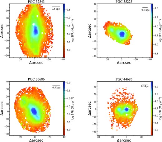
Spatially resolved SFR for PGC 32543, PGC 35225, PGC 36686, and PGC 44685, respectively. The physical scale corresponding to each arcsec is marked in the upper right corner of each panel.
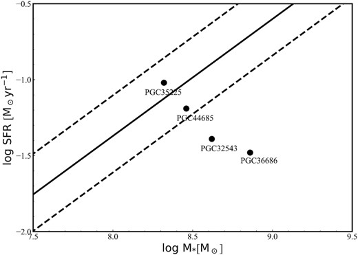
Star formation rate as a function of stellar mass. The black solid line indicating the star-forming main-sequence relation is adopted from Elbaz et al. (2007) and the dashed lines represent 68 per cent dispersion.
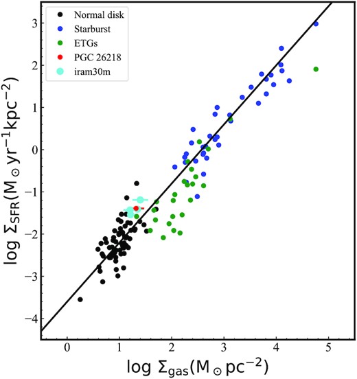
log Σgas versus log ΣSFR integrated over the beam size of the IRAM 30-m telescope (∼ 22 arcsec) for CO(J = 1–0). The objects with spatially resolved CO(J = 1–0) detections (green points) are from Davis et al. (2014), while normal (black) and starburst (blue) galaxies are from Kennicutt (1998b). The solid line represents the best fit for the Kennicutt (1998b) sample. The red point indicates a star-forming S0 galaxy that was studied by Ge et al. (2020). The sources observed by the IRAM 30-m telescope are marked in cyan.
Many studies have shown that there is an inverse correlation between |$\rm \alpha _{CO}$| and metallicity (Bolatto et al. 2008; Leroy et al. 2011; Sandstrom et al. 2013), because metallicity traces the total dust content that can shield CO from ultraviolet radiation. In this work, we adopt the |$\rm \alpha _{CO}$| of the Galaxy. However, considering that our sources are low mass/metallicity, this assumption may underestimate the molecular gas mass. In order to determine how the molecular gas mass changes, we estimate |$\rm \alpha _{CO}$| by using an empirical formula related to gas-phase metallicity and the distance off the main sequence given by Accurso et al. (2017). We find that the average |$\rm \alpha _{CO}$| of these S0 galaxies is 8.79 (from 6.15–12.33), which leads to Σgas being underestimated twice. Considering this conversion factor, which depends mainly on the metallicity, our sources will move an average of 0.3 dex to the right in the K–S law (although this will lead these S0 galaxies to follow this law better). However, the formula from Accurso et al. (2017) does not apply to galaxies merging or interacting with the environment (multiple star-forming regions). Therefore, whether we really underestimate the molecular gas mass needs additional clues. We note that the above results may have a selection effect, because these S0 galaxies were picked out via visual morphologies and B-band magnitude (Xiao et al. 2016). Ge et al. (2020) studied the physical properties of a nearby star-forming S0 galaxy (red point in Fig. 5) by combining optical and millimetre data. Their results indicated that this S0 galaxy might have experienced a minor merger, which triggered central star formation and resulted in a similar star formation efficiency to star-forming and starburst galaxies. Our result is consistent with that of Ge et al. (2020). Based on the existence of multiple star-forming regions, we suggest that the star formation of these S0 galaxies is probably related to a merger event (see Section 4 for a detailed discussion of this issue).
3.2 Kinematics of star and ionized gas
In Figs 6–9, we compare the kinematics of stars and Hα-emitting ionized gas. We note that we only select spaxels with signal-to-noise ratio (S/N) higher than 10, which will have reliable velocity measurements. We find that the velocity fields of stars (the shift of stellar absorption lines relative to the systematic velocity) of all sources are disorganized, which indicates that these star-forming S0 galaxies do not show structures characteristic of a rotating disc. Similarly, we find that the velocity fields of ionized gas (the shift of emission lines relative to the systematic velocity) do not show regular rotating structure, except for PGC 32543. We derive the axial ratios based on a two-dimensional, single-component Sérsic fit in the r band from the SDSS website2 \cite{2011AJ....142...31B}(Blanton et al. 2011) and find that the axial ratios for PGC 32543, PGC 35225, and PGC 36686 are approximately 0.51. This shows that these sources are not entirely face-on galaxies. On the other hand, PGC 44685 does not display a rotated disc-shape structure, probably because it is a blue compact dwarf analysed in Zhao, Gao & Gu (2013) or because it is a face-on galaxy based on the decomposition of bulge and disc (Xiao et al. 2016). In addition, we also find that the velocity dispersions of stars and ionized gas are low in regions with high star formation, which indicates that these star-forming S0 galaxies still have significant rotation. This is expected if these systems are starburst dwarfs.
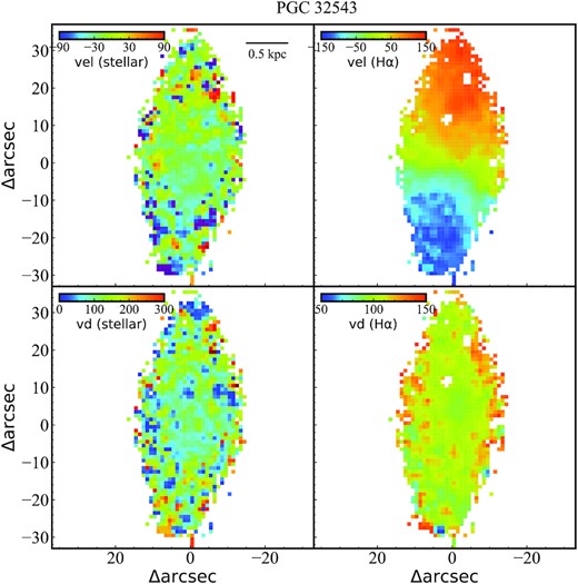
The distributions of kinematics for PGC 32543. The component of velocity is labelled in the upper left corner of each panel. Note that we only select spaxels with S/N higher than 10 to measure the stellar velocity. The physical scale corresponding to each arcsec is marked in the upper right corner of the first panel.

As for Fig. 6, but for PGC 35225.
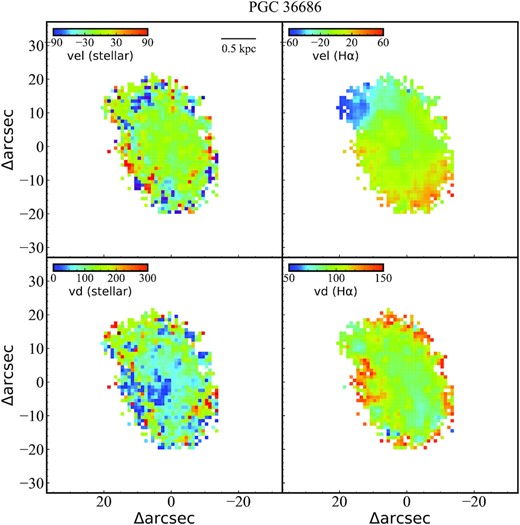
As for Fig. 6, but for PGC 36686.
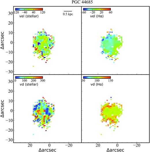
As for Fig. 6, but for PGC 44685.
3.3 Observation of cold gas
From the best-fitting CO emission lines in Fig. 10, we note that the four S0 galaxies have masses of molecular gas less than |$10^{7}~\rm M_{\odot }$|. In addition, the fraction of molecular gas (|$M_{\rm H_2}/M_{\ast }$|) is lowest at 0.8 per cent for PGC 32543 and highest at 1.5 per cent for PGC 35225. This result is consistent with their positions in the main-sequence relation (see Fig. 4). However, we find that the mass of atomic gas is about 1–2 orders of magnitude higher than that of molecular gas and is of the order of the stellar mass. Molecular gas arises mostly from the stellar mass returned to the galaxy, while atomic hydrogen is mainly accumulated from external sources (infall, captured dwarfs, etc.). In this work, for these dwarf S0 galaxies it is difficult to form stars by using the molecular hydrogen returned by stars, considering their low gravitational potential well. Therefore, the material for star formation is more likely to come from the external environment, where atomic hydrogen is easier to obtain. This is why the mass of atomic hydrogen is significantly greater than that of molecular hydrogen in our work. These discoveries suggest that the star-forming materials of these galaxies may be derived from their rich atomic gas. The source of this rich gas may be merger events (Davis et al. 2015) or the accretion of cold gas (Dressler et al. 2013).
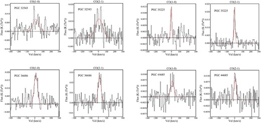
The observed CO(J = 1–0) and CO(J = 2–1) spectra centred on systemic redshifts taken from SDSS for our sample. The black and red lines represent the original spectra and single Gaussian model, respectively.
When the empirical formula from Schruba et al. (2018) is used, ΣHI may be underestimated, considering that these S0 galaxies may be accreting gas from the surroundings, therefore reducing the metallicity and thus the density of atomic hydrogen. In these cases, Σgas should move to a larger region. The other factor that may affect the estimation of Σgas is that we do not know how the gas is distributed. However, the resolution of CO(J = 1–0) produced by the IRAM-30 m telescope can basically cover the star-forming regions of these dwarf galaxies. Therefore, it would not change our results significantly.
We also find that the FWHM of CO(J = 1–0) is ≲ 100 km s−1, which might be caused by the concentration of gas in the centre. The disturbed discs of stars and ionized gas may also support this result. We utilize the Tully–Fisher relation (i.e. M* versus FWHM) given by Tiley et al. (2016) to estimate the FWHM of these S0 galaxies. However, the line widths of only two sources (PGC 32543 and PGC 44685) are consistent with our fitting results. The CO(J = 1–0) profile of PGC 35225 shows asymmetry, and there seems to be absorption on the left side of the emission line. This non-Gaussianity in shape may cause it to deviate from the Tully–Fisher relation. It noted that the relation between the stellar mass and FWHM of CO(J = 1–0) from Tiley et al. (2016) is based on a sample with M* ≳ 9.5. Whether low-mass S0 galaxies conform to this relationship needs to be verified by larger samples.
The line ratios between CO(J = 2–1) and CO(J = 1–0) (i.e. I21/I10) can be used to investigate the physical properties of molecular gas, although the emission from dense and diffuse surrounding molecular gas would complicate the interpretation. The line ratio is determined by the excitation temperature and spatial distribution of the cold gas. When the CO gas is compacted relative to the beam, then CO (J = 2–1) is stronger than CO (J = 1–0). However, if the distribution of CO emission is not dense enough, then the intensity of CO (J = 2–1) will be weakened more than that of CO (J = 1–0), which will result in a ratio of less than 1. The values of I21/I10 for PGC 32543, PGC 35225, PGC 36686, and PGC 44685 are 74, 69, 43, and 30 per cent, respectively. This result might indicate that the cold gas traced by different CO emission lines is either very diffuse or has significantly different excitation temperatures. Some previous studies (Li, Seaquist & Sage 1993; Sage 1990; Wiklind et al. 1997) have shown that 0.5 ≲ I21/I10 ≲ 1.0 implies that the gas is optically thick. In addition, a study in |$\rm ATLAS^{3D}$| has shown that the integrated CO (J = 2–1)/CO (J = 1–0) of ETGs ranges from 1 to 4 (Young et al. 2011). The difference between this work and Young et al. (2011) may be caused by either subthermal excitation or pointing errors that cause the intensity of the CO(J = 2–1) line to be underestimated. We find that objects with high ratios of integrated intensity have low SFR (e.g. PGC 32543), while objects with low ratios have relatively high SFR (e.g. PGC 44685). Such a contradiction may be related to telescope–beam coupling and the inevitable mixing of emission from dense and diffuse molecular gas. A larger sample is needed to investigate the relationship between the ratio of different transitions and star-forming activity.
4 DISCUSSION
In broad terms, galaxies could form via either monolithic formation or hierarchical accumulation. In the monolithic formation mechanism, a large amount of gas collapses rapidly to form galaxies. The speed of gas collapse determines whether elliptical, S0, or spiral galaxies with a spheroidal bulge are formed (Arimoto & Yoshii 1987; Rocca-Volmerange & Guiderdoni 1988; Bower, Lucey & Ellis 1992; Bruzual & Charlot 1993). S0 galaxies are generally thought to have formed most of their stellar mass 10 Gyr ago, which is why they are quiescent at present. This view has been reinforced by the paucity of atomic gas (Wardle & Knapp 1986) and star-forming regions (Pogge & Eskridge 1993). Welch & Sage (2003) studied the relation between the total mass of atomic and molecular gas and blue luminosity of S0 galaxies and they found that S0 galaxies have lost almost 90 per cent of their gas. However, the main disadvantage of this theory is that the massive protogalaxies that should be observed have not been observed at any redshift. In addition, S0 galaxies formed in this way should have a bulge component and have little star formation. In our sample, we do not find that these S0 galaxies have a large Sérsic index. As Xiao et al. (2016) pointed out, S0 galaxies with star formation have lower Sérsic index than those without star formation. The deficiencies in monolithic formation have stimulated investigations of the hierarchical formation idea, where galaxies grew their stellar mass through a series of merger events (White & Frenk 1991; Kauffmann, White & Guiderdoni 1993; Baugh, Cole & Frenk 1996). Clumps of different mass and angular momentum interact, which may lead to continuous star formation. At the same time, the evolution of galaxies will continue for a long time, and even at the present epoch we may see the relics of interaction (e.g. multiple star-forming knots).
The study from Kaviraj (2014) showed that ETGs host about 14 per cent of the star formation budget caused by minor merger events. This indicates that minor mergers may play an important role in driving star formation and leading perturbed stellar morphology. Based on a toy model, Davis & Bureau (2016) found that a high gas-rich merger rate may be required to explain more efficient star formation in local ETGs. Considering that the major-merger rate is significantly lower than the minor-merger rate (Lotz et al. 2011), gas-rich minor mergers dominate the accretion of cold gas (Kaviraj et al. 2011). For these star-forming S0 galaxies, they are morphologically disturbed (e.g. star-forming knots) and have turbulent kinematics, which supports the picture in which minor mergers can be a dominant factor for star formation in later morphological types.
The metal content is a fundamental tracer of the star formation history. Grossi et al. (2020) studied two star-forming dwarf galaxies in the Virgo cluster and found that these galaxies show positive gas metallicity gradients. They suggested that the dilution of gas-phase metallicity is associated with a recent merging event. In Fig. 11, we show the spatially resolved oxygen abundance and radial distributions of oxygen abundance for our sample. We find that the oxygen abundance in star-forming regions is lower than that of the outside area. Although the oxygen abundance estimates have large errors, we also find from the radial distributions of oxygen abundance that the oxygen abundance of these S0 galaxies increases with increasing radius, showing a trend of positive metallicity gradients. This result is consistent with Grossi et al. (2020). Combined with the multi-nuclear structure and rich atomic gas, we suggest that the hierarchical accumulation paradigm might be an indication for star formation in very low-mass S0 galaxies.
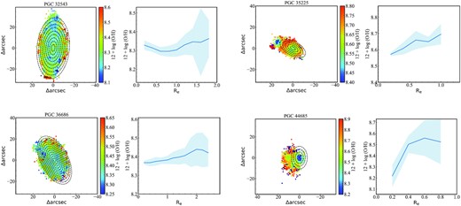
Left: spatially resolved oxygen abundance for PGC 32543, PGC 35225, PGC 36686, and PGC 44685 for spaxels with S/N higher than 10. Right: radial distributions of oxygen abundance and errors (the average oxygen abundance and the standard deviation in each circle).
5 SUMMARY
In this work, we focus on the spatially resolved properties and cold gas content of four dwarf S0 galaxies with multiple cores based on optical IFS observations from CAHA and millimetre observations from IRAM-30 m. The main results are summarized as follows.
We find that all the sources in our sample (except PGC 35225, which has the highest ratio of molecular gas to stellar mass) have deviated from the SFMS relation or are in the process of deviating from this relation. However, these S0 galaxies follow the K–S law within the star-forming region, which indicates that the star formation of dwarf S0 galaxies may be more extended.
In the velocity field distribution of star and ionized gas, we do not find regular rotating structures. Such disturbed kinematics suggests that star formation in these S0 galaxies may be triggered by galaxy mergers or other external environmental effects. This picture is consistent with the multiple star-forming knots in our galaxies. We find that the star-forming knots have lower velocity dispersions of stars and ionized gas, which indicates that dwarf S0 galaxies still have significant rotation. The result is supported by the fact that most of these dwarf S0 galaxies are classified as fast rotators.
The physical properties of molecular gas of these dwarf S0 galaxies are very complicated. Their line ratios I21/I10 are all less than 1.0, which indicates that the distributions and excitation temperatures of different CO transitions are very different.
We have detected molecular gas in all of these S0 galaxies, with molecular gas accounting for between 0.8 and 1.5 per cent of the stellar mass. Although the content of molecular gas is very limited, we find that they store a lot of atomic gas, the mass of which is almost comparable to the stellar mass. In addition, the relation between gas-phase metallicities and SFR shows an inverse correlation, i.e. the richer the metal content, the lower the SFR. We suggest that abundant atomic gas in these low-mass S0 galaxies may come from a series of mergers and/or accretion events. It was this rich atomic gas, combined with a long dynamical time-scale (fast rotator), that led to extended star formation history in these dwarf S0 galaxies in a field environment. However, further observations are needed to confirm whether the atomic gas reservoirs belong to these galaxies.
ACKNOWLEDGEMENTS
We are very grateful to the anonymous referee for critical comments and instructive suggestions, which significantly strengthened the analyses in this work. This work is supported by the National Key Research and Development Program of China (No. 2017YFA0402703) and by the National Natural Science Foundation of China (No. 11733002). In addition, we acknowledge the support of the staff from CAHA and IRAM-30 m. RGB acknowledges additional financial support from the State Agency for Research of the Spanish (MCIU) through the Center of Excellence Severo Ochoa award to the Instituto de Astrof\'isica de Andaluc\'ia (SEV-2017-0709), grants PID2019-109067GB-I00 (MCIU), and P18-FRJ-2595 (Junta de Andaluc\'ia). We are grateful for the support of the scientific research fund of Jiangsu Second Normal University (927801/032). N.D acknowledges financial support from the National Natural Science Foundation of China grant 12103022 and the scientific research fund of Yunnan Provincial Education Department (2021J0715).
DATA AVAILABILITY
The data underlying this article cannot be shared publicly due to the privacy of individuals that participated in the study. The data will be shared on reasonable request to the other authors.
