


ABSTRACT
Since 2005 December, recurrent outbursts have been observed for Centaur 174/P Echeclus, confirming it is an active object. Thanks to a large number of photometric data obtained between 2001 April and 2019 December, we were able to compute a shape model of this object. We obtain a sidereal rotation period P = 26.785178 ± 10−6 h and six equally probable pole solutions, each with a large obliquity of the rotational axis (50° or more). We also find the object significantly elongated, with a semi-major axial ratio a/b = 1.32 (and b/c ∼ 1.1 but this second ratio is poorly constrained by the photometric data). Additionally, we present a detailed analysis of the dust emission from the 2016 outburst. Different colour maps are presented that reveal a change in dust colour, which becomes bluer with increasing cometocentric distance. A blue ring-like structure around the nucleus clearly visible in the images obtained on October 4 in the V-R spectral interval points out that the innermost near nucleus region is considerably redder than the surrounding coma. Different jets are also apparent, the main one being oriented southward. A detailed dynamical study is done to investigate past and future orbital elements. These elements appear stable in the period ≈1200 CE to ≈2900 CE. For a period of 12 000 yr the main conclusion is that Echeclus’ perihelion distance was greater than about 4 au, preventing it from following a typical cometary activity like a short-period comet. Close encounters with giant planets nevertheless prevent any study of orbital elements on longer timescale.
1 INTRODUCTION
Among the different categories of small bodies belonging to the Solar system, centaurs are representative of transitional objects coming from the population of Kuiper belt objects (KBOs). They are scattered inward on to unstable orbits with dynamical lifetimes around 106–107 yr, some of them becoming Jupiter family comets (JFCs) (Tiscareno & Malhotra 2003; Horner, Evans & Bailey 2004; Di Sisto & Brunini 2007; Sarid et al. 2019). Their orbits are conventionally defined to have a perihelion greater than Jupiter’s semimajor axis (5.2 au) and a semi-major axis smaller than that of Neptune (30 au). About 13 per cent of these objects display comet-like activity (Jewitt 2009).
In this context, studying active centaurs is important for a better understanding of the origin of JFCs. Centaurs often present unpredictable outbursts not necessarily correlated with their perihelion distance. (60558) 174P/Echeclus, initially designated as 2000 EC98 (hereafter Echeclus), is a well-known active centaur characterized by four large outbursts in 2005, 2011, 2016, and 2017, as well as one detected on pre-discovery Spacewatch images obtained in 2000 January (Choi & Weissman 2006). Its heliocentric distance varies between 5.81 and 15.61 au with a period of 35.06 yr, the last perihelion passage being on 2015 April 23.1
Echeclus is a small centaur discovered by the Spacewatch program on 2000 March 3 (Marsden 2000). It has a diameter of D = 64.6 ± 1.6 km and an albedo of 5.20|$^{+0.70}_{-0.71}$| per cent, based on data from Spitzer and Herschel space observatories (Duffard et al. 2014). The colours of centaurs (or spectral slopes) follow a bimodal distribution with a red group and a less-red group (Peixinho et al. 2003; Barucci et al. 2005; Tegler et al. 2008; Perna et al. 2010). Echeclus has no ice absorption features (Guilbert et al. 2009; Seccull et al. 2019) and is more steeply red at visible wavelengths compared to near-infrared ones as is typical to the less-red group of centaurs. All but one active centaurs [523676 (2013 UL10), Mazzotta Epifani et al. (2018)] belong to the less-red group.
The main outburst was detected in 2005 December 30 (Choi, Weissman & Polishook 2006a), when the overall V magnitude decreased from ∼21 to ∼14 while Echeclus was at preperihelion, 13 au from the Sun. This outburst was observed both in the optical and infrared range (Choi et al. 2006b; Choi, Weissman & Polishook 2006c; Choi & Weissman 2006; Weissman et al. 2006; Bauer et al. 2008; Rousselot 2008) showing that the centre of brightness of the cometary activity was not on the nucleus itself, but offset by about 1.4–8 arcsec, depending of the date of observations (2005 December–2006 March). Some authors suggested that this unusual coma appearance could be due to the ejection of a fragment, this fragment being the source of cometary activity (Choi et al. 2006b; Weissman et al. 2006; Fernández 2009). Another modelling also based on archive data obtained on 2005 December 22, suggests that this outburst could be explained by two short events (a few hours each) coming from 2 localized point sources on the nucleus followed by a longer from a third source (Rousselot et al. 2016). This modelling also suggest a high obliquity for the rotation axis. Visual and infrared observations conducted in 2006 February showed a dust-particle size distribution of large grains consistent with a typical steady cometary activity and different from what would be expected by an impact driven event, such as the one observed by the Deep Impact experiment (Bauer et al. 2008). Spectroscopic observations performed in the optical range could not detect gaseous emission lines and only an upper limit could be obtained for the C2 and CN radicals (Rousselot 2008).
The main outburst observed in 2005 was followed by three smaller ones: in 2011 May (Jaeger et al. 2011) with 2–3 visual magnitude brightening, 2016 August (Miles et al. 2016) with 2.5–3 visual magnitude brightening and 2017 December with 4-4.5 visual magnitude brightening (this last one being first reported online by Brian Skiff (Lowell Observatory) on December 7.2 Observations performed during the 2016 outburst revealed an unusually blue dust coma, which may be indicative of a carbon-rich dust composition but no discernible absorption features in the spectrum could be observed (Seccull et al. 2019). A very faint CO emission line was also observed in the submillimeter range at 6 au from the Sun, with scans accumulated on Echeclus in the period 2016 May 28 – June 9, corresponding to an heliocentric distance of 6.1 au (Wierzchos, Womack & Sarid 2017).
Near-infrared and visible observations performed during the last outburst, in 2017 December by Kareta et al. (2019) revealed a bluer dust coma than Echeclus itself, consistent with previous observations performed by Seccull et al. (2019). A secondary peak - which was hinted at in the visible images – was also observed in the near-infrared 2D spectra. It was interpreted as being due to a collection of material up to a few meters in size ejected approximately in the same direction from the nucleus at a speed of about 21–23 m s−1.
Some photometric data covering the period 2001–2016 revealed significant changes in the light-curve amplitude varying from 0.24 in the R-band (Rousselot et al. 2005) to no detectable light-curve in 2013 July (Rousselot et al. 2016). Such variations, additionally to the modelling of the main outburst, seem to indicate a large obliquity for the nucleus rotational axis.
This paper presents, for the first time, a shape model of Echeclus, based on the already large data set presented in Rousselot et al. (2016) improved with new observational data. Some new observational data of the outburst observed in 2016 are also presented as well as a dynamical study of Echeclus. Section 2 presents the observational data, Section 3 details the shape model obtained from these data, Section 4 the observational data obtained during the 2016 outburst, Section 5 the dynamical history of Echeclus, and the results are discussed in Section 6.
2 OBSERVATIONAL DATA
The data set used in this paper comprises observations gathered during six observing periods (2001, 2002, 2003, 2013, 2016–2017, and 2019) performed with different telescopes. The main technical parameters of the telescopes and CCD detectors are presented in Table 1 and the observing circumstances are summarized in Table 2. Three other observing periods were connected with outbursts of Echeclus in 2005, 2011, and 2016. The 2001, 2002, 2003, and 2013 observations have already been described in Rousselot et al. (2016). The new data gathered in 2016–2017 and 2019 have not been published yet, they are described below.
Equipment used for the observations (for the observational data corresponding to images). NOT: Nordic Optical Telescope (La Palma). LT: Liverpool Telescope (La Palma). CFHT: Canada-France-Hawaii Telescope. VLT: Very large Telescope (ESO). NTT: New Technology Telescope (ESO). Danish: Danish Telescope (ESO). T 3.6-m: 3.6-m telescope (ESO). RBT/PST2: Roman Baranowski Telescope/Poznan Spectroscopic Telescope 2 (Arizona, USA).
| Telescope | Diameter | Instrument | CCD | Scale | Field of view | Filter |
|---|---|---|---|---|---|---|
| (m) | (arcsec/pix) | (arcmin×arcmin) | ||||
| NTT | 3.58 | SUSI 2 | 2 × 2048 × 4096 | 0.0805 (binned 2 × 2) | 5.5 × 5.5 | B,V,R |
| 3.6-m | 3.57 | EFOSC2 | 2048 × 2048 | 0.157 (binned 2 × 2) | 5.4 × 5.4 | B,V,R |
| Danish | 1.54 | DFOSC | 2048 × 4096 | 0.39 | 13.7 × 13.7 | B,V,R |
| NOT | 2.5 | ALFOSC | 2048 × 2048 | 0.19 | 6.5 × 6.5 | B,V,R,I |
| LT | 2.0 | IO:O | 4096 × 4112 | 0.15 (binned 2 × 2) | 10 × 10 | B,V,r’ |
| Aristarchos | 2.3 | LN2 CCD | 2048 × 2048 | 0.16 (binned 2 × 2) | 5.5 × 5.5 | B,V,R,I |
| VLT | 8.2 | FORS2 | 2048 × 2048 | 0.25 | 6.8 × 6.8 | B,V,R,I |
| RC | 2.0 | 2084 × 2084 | 0.31 (binned 2 × 2) | 10.8 × 10.8 | B, V, R | |
| RBT/PST2 | 0.7 | Andor iXon X3 | 1024 × 1024 | 0.59 | 10 × 10 | L |
Observing circumstances (by chronological order of the observations). r: heliocentric distance (au); Δ: geocentric distance (au); α: phase angle.
| UT Date | r | Δ | α | Filter | Telescope | Comment |
|---|---|---|---|---|---|---|
| 2001 April 26 | 15.16 | 14.46 | 2.8° | B,V,R | NTT | See Rousselot et al. (2005) |
| 2001 April 27 | 15.16 | 14.47 | 2.9° | B,V,R | NTT | See Rousselot et al. (2005) |
| 2002 March 18 | 14.90 | 13.90 | 0.1° | B,V,R | Danish | See Rousselot et al. (2005) |
| 2002 March 19 | 14.90 | 13.90 | 0.2° | B,V,R | Danish | See Rousselot et al. (2005) |
| 2002 March 23 | 14.89 | 13.90 | 0.4° | B,V,R | Danish | See Rousselot et al. (2005) |
| 2002 March 24 | 14.89 | 13.90 | 0.5° | B,V,R | Danish | See Rousselot et al. (2005) |
| 2003 April 10 | 14.50 | 13.55 | 1.4° | B,V,R | T 3.6-m | See Rousselot et al. (2005) |
| 2003 April 11 | 14.49 | 13.56 | 1.4° | B,V,R | T 3.6-m | See Rousselot et al. (2005) |
| 2003 April 12 | 14.49 | 13.56 | 1.5° | B,V,R | T 3.6-m | See Rousselot et al. (2005) |
| 2013 July 4 | 6.59 | 5.57 | 0.9° | B,V,R,I | NOT | See Rousselot et al. (2016) |
| 2013 Juy. 5 | 6.58 | 5.57 | 0.8° | B,V,R,I | NOT | See Rousselot et al. (2016) |
| 2013 July 6 | 6.58 | 5.57 | 0.8° | B,V,R,I | NOT | See Rousselot et al. (2016) |
| 2013 July 7 | 6.58 | 5.57 | 0.7° | B,V,R,I | NOT | See Rousselot et al. (2016) |
| 2013 July 8 | 6.58 | 5.56 | 0.7° | B,V,R,I | NOT | See Rousselot et al. (2016) |
| 2016 September 12 | 6.30 | 5.42 | 4.89° | B,V,R,I | VLT | This work |
| 2016 September 22 | 6.32 | 5.37 | 3.38° | B,V,R,I | VLT | This work |
| 2016 October 01 | 6.33 | 5.35 | 1.81° | B,V,R | RC | This work |
| 2016 October 02 | 6.33 | 5.35 | 1.66° | B,V,R | RC | This work |
| 2016 October 03 | 6.34 | 5.35 | 1.49° | B,V,R | RC | This work |
| 2016 October 04 | 6.34 | 5.35 | 1.43° | B,V,R,I | VLT | This work |
| 2016 October 04 | 6.34 | 5.35 | 1.33° | B,V,R | RC | This work |
| 2016 October 05 | 6.34 | 5.35 | 1.16° | B,V,R | RC | This work |
| 2016 October 06 | 6.34 | 5.35 | 1.00° | B,V,R | RC | This work |
| 2016 October 07 | 6.34 | 5.35 | 0.85° | B,V,R | RC | This work |
| 2017 January 20 | 6.54 | 6.70 | 8.42° | B,V,R,I | Aristachos | This work |
| 2017 January 21 | 6.55 | 6.72 | 8.38° | B,V,R,I | Aristachos | This work |
| 2017 January 22 | 6.55 | 6.73 | 8.35° | B,V,R | RC | This work |
| 2019 December 17 | 9.26 | 8.29 | 1.04° | L | RBT/PST2 | This work |
| 2019 December 20 | 9.27 | 8.31 | 1.34° | L | RBT/PST2 | This work |
| 2019 December 30 | 9,29 | 8.38 | 2.40° | L | RBT/PST2 | This work |
2.1 2016-2017 data set from Peak Terskol observatory
Echeclus was observed with the 2-m Ritchey-Chretien Telescope (RC) of Peak Terskol observatory operated by the International Center of Astronomical, Medical and Ecological Research of the National Academy of Sciences of Ukraine (Terskol, Kabardino-Balkaria, Russia) in 2016 October, approximately one month after the outburst, and in 2017 January. In 2016, the observations were obtained over the course of seven nights; one night of the observations in 2017 followed immediately the observing run performed in Helmos observatory (see below). During this observing run we were able to provide field images for the data taken at Terskol observatory for photometric calibration, as explained below in Section 2.2 (see Table 2).
For the observations at Peak Terskol we used a 2084 × 2084 CCD detector with a pixel size of 24 × 24 μm mounted in the Cassegrain focus of the RC. It provides an image scale of 0.62 arcsec per pixel on the sky and a field of view of about 10.8 × 10.8 arcmin in a 2 × 2 binned mode. Sequences of B, V, R -images of the target with single exposures of 60–120 s depending on the filter used were obtained during each night. Several Landolt fields provided standard stars for the absolute photometric calibration. In addition to the images of the target, a set of bias and flatfield images were taken for the routine preprocessing procedure.
Since Echeclus’ rotation period has been estimated at about 26.8 h, assuming a double-peaked light-curve (Rousselot et al. 2005), we observed the target at each of 7–8 consecutive nights starting observations at approximately the same UT moment in order to cover entire light-curve. However, not all the nights were photometric, therefore, we decided to utilize background stars from the photometric catalogue APASS (The American Association of Variable Star Observers Photometric All-Sky Survey)3 for the absolute photometric calibration. The catalogue contains stars with magnitudes between 7 and 17 measured in five band passes: B, V Johnston-Cousins, Sloan g′, r′, i′. The photometric uncertainties of the catalogue are in the interval 0.03–0.11 mag depending on star brightness (Henden et al. 2011). In order to transform the APASS r′ magnitudes to the Johnson-Morgan-Cousins system we used the expression taken from Fukugita et al. (1996).
In order to test possible systematic bias in magnitudes that could arise from usage of the APASS catalogue as a reference, we re-calculated magnitudes of APASS stars in the Landolt system and compared them with the original ones. The Landolt fields were observed in a wide range of airmasses and provided zero points, extinction, and colour terms for each filter used with errors inferior to 0.02 mag. For three nights of good photometric quality no systematic differences between original APASS magnitudes and those calculated with the Landolt fields were found at the level of a root mean square error of approximately 0.02 mag. This confirmed the quality of photometric calibration with APASS stars. Therefore we used three to seven stars in each image to calculate the magnitudes of Echeclus. As previously stated the images obtained in 2017 were calibrated with the field stars provided by the data obtained with the Aristarchos Telescope (see below).
Aperture photometry was applied to extract fluxes from the target and standard stars. A circular aperture with a small radius (less than 3×FWHM) was used for the flux integration to avoid contamination from the slight coma visible around Echeclus in the images obtained in 2016. In 2017 Echeclus had a star-like appearance, therefore an aperture of about 3×FWHM was applied. Photometric error of Echeclus’ magnitudes was estimated as a sum |$\sigma = (\sigma ^{2}_{stat}+\sigma ^{2}_{stand})^{1/2}$|, where σstat and σstand are the statistical error, dominated by background uncertainty, and the error of the magnitude of a standard star, taken from the APASS catalogue. To evaluate σstat the SNR equation was taken from Merline & Howell (1995). The noise model takes into account the number of pixels in the apertures used for target and background integration as well as the readout noise. Typically, σstat was less than 0.02 mag and σstand varied between 0.01 mag and 0.1 mag. Since several stars were used for the flux calibration, we excluded those with large photometric uncertainty. Resulting photometric accuracy of the target magnitudes is between 0.03 and 0.07 mag for most of the nights.
2.2 2017 data set from Helmos observatory
A total of three observing nights [9 × 0.3 nights (beginning)] were allocated to the 2.3-m Aristarchos telescope located at Helmos observatory (Greece) for the period 2017 January 16–25. Due to poor weather observations were performed only during two consecutive early nights of both January 20 and 21.
The images were obtained with the LN2 CCD optical CCD imaging camera. The field of view of this instrument is 5.5 × 5.5 arcmin using a 2048 × 2048 CCD detector with a 0.16 arcsec pixel size on the sky. Because of a 2 × 2 binning mode the real scale was 0.32 arcsec.pixel−1. Broad-band BVRI filters were used with 60-s exposures time, half of the images being obtained with the R-band filter. A field with standard stars was also observed at different airmasses to provide information for the photometric reduction. The seeing value was about 2 arcsec during the first night (January 20) and 0.8 arcsec during the second (January 21). The images were preprocessed using a bias and a master sky flat-field obtained during the observing run.
The photometric analysis of Echeclus was done using a two-step process. In a first step a complete photometric reduction (i.e. computation of the photometric coefficients) was done for both nights, thanks to standard stars images obtained at different airmasses. These photometric coefficients allowed the computation of the real BVRI magnitudes of three different stars chosen as reference stars appearing in the field of view of January 20, 21 and 22 (these three fields of view being observed during the same night, on January 21). In a second step relative photometry was conducted for the nights of January 20 and 21, between Echeclus itself and the reference stars. It allowed the computation of the real apparent BVRI magnitudes of Echeclus. Thanks to the reference stars observed with the Aristarchos telescope during the night January 21 it was also possible to compute the apparent real magnitude with the R filter for the observational data obtained on January 22 with the 2-m Peak Terskol telescope. A light-curve is clearly visible from these data, with an amplitude that can be estimated to about 0.4 ± 0.1 mag when Peak Terskol data are taken into account (Fig. 1).
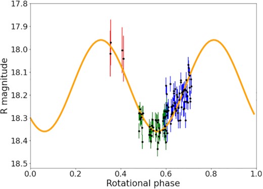
Light-curve obtained with Helmos observations performed in 2017 January 20, 21 (respectively blue and green) mixed with one obtained at Pik Terskol observatory on 2017 January 22 (red). Superimposed is a sinusoidal variation with an amplitude of 0.4 mag.
2.3 2019 data set from Winer observatory
Photometric observations during 2019 opposition were obtained over the course of 3 nights in 2019 December with RBT/PST2 0.7 m telescope (Planewave CDK700) located in Winer Observatory (Arizona, USA). An Andor iXon X3 888 back-side illuminated 1024 × 1024 EMCCD camera with L filter was used. The L filter used at the RBT/PST2 telescope is an interferometric luminosity filter with a transmission window from 3700 to 7000 Å. The camera, with a pixel size of 13 × 13 μm, was mounted on the Nasmyth focus of the telescope providing an image scale of 0.59 arcsec per pixel on the sky and a field of view of about 10 × 10 arcmin. All frames were exposed 300 s. After standard preprocessing for bias and flat-field an aperture photometry was carried out using PHOTOM programme included in the Starlink package. Composite light-curve Fig. 2 shows very low amplitude of brightness variations and confirms previously determined synodic period of 26.802 h (Rousselot et al. 2005).
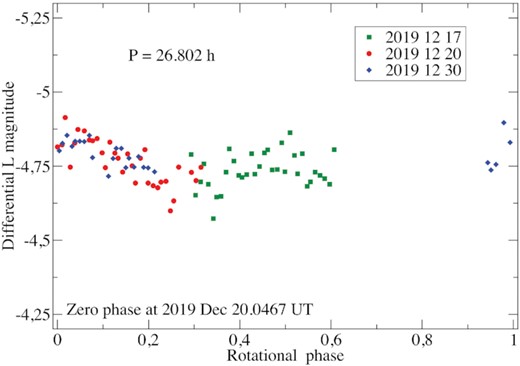
Composite light-curve of Echeclus obtained at RBT/PST2 in December 2019.
Because of poor weather conditions no calibration to the standard system was performed.
To confirm the absence of cometary activity during these observations we co-added the best 23 frames obtained on 2019 December 30. The final co-added image (Fig. 3), corresponding to an exposure time of 6900 s did not show any coma around Echeclus.
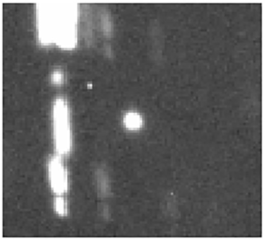
Co-addition of 23 frames obtained on 2019 December 30. No cometary activity is visible.
3 SHAPE MODEL
Light-curves obtained between the outbursts served as input data for the spin vector and shape modelling of Echeclus. We used 27 light-curves collected during almost 20 ys from 2001 to 2019. In the case of centaurs covering different observing geometries is a very time consuming process. Positions of Echeclus for the different epochs of photometric observations are shown in Fig. 4.
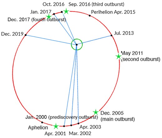
Orbit of Echeclus (red) with its positions at different epochs corresponding to the photometric observations. Orbit of the Earth is marked as green circle. Green stars highlight the different outbursts.
The model of Echeclus was created using SAGE modelling technique (Bartczak & Dudziński 2018), which is a light-curve inversion method based on a genetic algorithm. In the evolution-mimicking process a global minimum is searched for giving a non-convex shape model of an asteroid, its spin axis orientation, and rotational period. A constant albedo of the surface and homogeneous mass distribution inside the body are assumed. The minimization starts with a spherical body and a random spin axis. In each iteration a population of offspring models is created by introducing small and random changes to the parent model’s parameters. For each offspring a set of synthetic light-curves is calculated and compared to the observed ones. The rotational period is fitted individually for each offspring to assure the best fit. The model that does the best job of explaining observations is selected as the parent for the subsequent iteration. The process is stopped when the models do not change significantly from one iteration to the next. The whole process is performed multiple times to assure that the global minimum was found.
Even though the collected data covered multiple apparitions and variety of longitudes, the modelling of Echeclus proved to be quite challenging, primarily due to the long sidereal rotational period P = 26.785178 ± 10−6 h. In such a case observing a complete light-curve from a ground-based observatory in a single night is impossible. As seen in Fig. 5 we only had partial light-curves covering 1/3 of the rotation phase in the best case.

Some of the light-curves used in our shape model.
Light-curve inversion assumes homogeneous albedo. It is possible to introduce multiple patches of lower albedo on the surface, or treat the albedo of each triangle as a separate free parameter during the modeling. However, the number of the degrees of freedom of the model would then become too large for the algorithm to produce a solution in a reasonable time. Moreover, the albedo variation and the shape both impact the light-curves, and it is impossible to disentangle the contribution of either using visual photometry alone. For those reasons, brightness variation of the model presented in this work is explained only by the shape. However, it must be emphasized that Echeclus’ albedo could have changed from one apparition to another. Some parts of the surface might have been covered by newly ejected material, or sub-surface material got exposed. Given the fact, that the outbursts were indeed observed (see section below), it stands as a plausible scenario. This means that light-curves are not necessarily consistent with each other under the assumptions made during the modelling process, which could contribute to the large uncertainty of the pole solution.
The resulting shape model is shown in Fig. 6. It is a compromise that provided 6 pole solutions found during the modelling process, each of them being equally probable. The details of these pole solutions are given in Table 3. The map of solutions found during the modelling process is shown in Fig. 7. These values confirm that, in any case, the obliquity of the rotation axis is important, as it was already pointed out from the large variations of light-curve amplitude observed between 2001 and 2013.
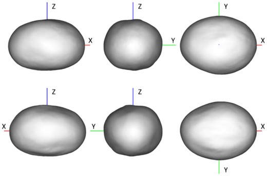
Projections of Echeclus’ model in xz, yz and xy planes.
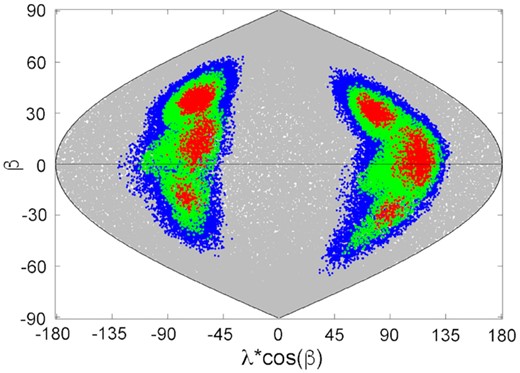
Pole solutions map obtained during the modelling process. The red colour marks solution with root mean squared deviation (RMSD) within 1 per cent from the best solution, green – 5 per cent, blue – 10 per cent.
Pole solutions provided by our shape modelling. λ represents the ecliptic longitude and β the ecliptic latitude. All these pole solutions are equally probable.
| Pole Solution | λ | β |
|---|---|---|
| 1 | −63 | 37 |
| 2 | −63 | 14 |
| 3 | −73 | −19 |
| 4 | 80 | 30 |
| 5 | 116 | 2 |
| 6 | 90 | 28 |
| Pole Solution | λ | β |
|---|---|---|
| 1 | −63 | 37 |
| 2 | −63 | 14 |
| 3 | −73 | −19 |
| 4 | 80 | 30 |
| 5 | 116 | 2 |
| 6 | 90 | 28 |
The shape of Echeclus is very close to a 3-axial ellipsoid. By comparing the areas of model’s projections we found semi-major axes ratios to be a/b = 1.32, b/c = 1.1. It has to be stressed that the b/c ratio is very unreliable as the extent of the model along its spin axis varied greatly over the course of the modelling.
4 2016 OUTBURST OBSERVATIONS
We performed observations of Echeclus with the 8.2-m VLT of ESO with the FOcal Reducer/low dispersion Spectrograph 2 (FORS 2) instrument. Three times 0.5 hours of observations were allocated to observe Echeclus during its 2016 outburst on 2016 September 12, 22 and October 4. Broad band B,V,R,I filters were used. Fig. 8 presents an overview of the images obtained in the R filter for each of these observing runs (coadded images).
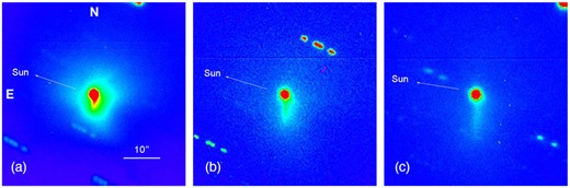
Outburst observed in 2016 with FORS2 at VLT (R band). A: 2016 September 12, B: 2016 September 22, C: 2016 October 4. At that geocentric distance 10 arcsec represents about 39 000 km.
We performed absolute calibration of the images with the Stetson standard fields observed during each night in a wide range of airmass. Additionally, approximately 8–10 field stars from the SDSS catalogue were chosen as standards and measured in each individual frame with the Echeclus image. The SDSS magnitudes of these intermediate standards were transformed into the Johnson-Cousins system with Lupton transformation equations.4 Atmospheric condition was stable enough during the observing runs with the seeing at level of 1.0 arcsec. The photometric coefficients (zero points, extinction and colour coefficients) derived during three observing periods are in agreements at level of 2 per cent–4 per cent depending on the colour band. There is also a good consistency in the colour coefficients extracted with the Stetson standards and the SDSS stars used as standards.
The asymmetric appearance of the coma image seen in Fig. 8 (the left-hand panel) suggests the possible presence of faint jet-like features hidden in the cometary coma. Therefore, we used the LarsonSekanina image processing technique to remove the bright central condensation accentuating more subtle variations of coma brightness (Larson & Slaughter 1992). The coadded images obtained through each filter used and for each observing run were processed with the Larson-Sekanina filter. For the same observing run the processed B, V, R, I-band images reveal the similar morphology of the faint jet-like features, therefore the enhanced R-band images obtained on three different epochs are presented in Fig. 9 as an example. Four faint jet-like features can be identified in the image obtained on September 12 and only one of them, which is directed to the south, is clearly observed in the images taken on the nights of September 21 and October 4. Two short rays seen in the right panel of Fig. 9 are probably artefacts due to image processing techniques. The applying another algorithms, namely, the ‘1/r division’ and ‘median subtraction’, confirms the southward jet only.

The coadded R-images of 174P/Echeclus enhanced with the Larson-Sekanina digital filter A: obtained on 2016 Sept. 12; B: on 2016 Sept. 22; and C: on 2016 Oct. 4. The arrows indicate four jet-like features, two spurious features are also marked with arrows in the right panel.
The variation of coma brightness was examined with the surface brightness radial profiles, which provided information about the variation of the grain column density along the line of sight as a function of projected distance from the comet nucleus. The radial profiles were constructed by averaging the coma flux values within concentric annuli of increasing radii centred on the Echeclus’ photometric centre. The slope of the surface brightness was calculated by fitting the logarithmic dependence ‘log(B)-log(ρ)’ (Jewitt & Meech 1987). In this expression, B is the azimuthally averaged surface brightness within the annular aperture, measured in units of the mean solar disk intensity (Arvesen, Griffin & Pearson 1969), and ρ is the outer annular radius projected in the sky-plane at the comet distance and expressed in km. Fig. 10 shows the brightness radial profiles produced from the R-band images taken over three observing nights. A simple model of a cometary coma with the constant source of dust grains leaving a nucleus at constant velocity implies that the volume density of emitted grains is inversely proportional to the squared distance from the nucleus. In this case the azimuthally averaged radial profile is expected to decrease as a ρ−1. The steeper profiles indicate that coma grains are accelerated by solar radiation pressure or sublimation from the grains themselves; the outer coma regions can become highly distorted by radiation pressure and the surface brightness gradient drops steeper than −1.5 (Jewitt 2004; Baum, Kreidl & Schleicher 1992). The majority of surface brightness profiles observed for other comets become steeper with increasing distance from the nucleus (Jewitt & Meech 1987). As seen in Fig. 10, a single linear fit does not represent properly the logarithmic dependence of Echeclus’ surface brightness in the full range of projected distances. For the night of September 12, the brightness profile is very shallow (slope = −0.63) within distances of about 21,400 km, becoming steeper at larger distances from the nucleus. There is a dissimilarity between the profiles produced from the images acquired over the nights of September 21 and October 4: they become shallower in the outer coma region. A profile with a slope less than unity can be caused by the presence of a source function in the cometary coma, e. g. the grain fragmentation. The change in the radial profiles of Echeclus’ brightness seen between September 21 and October 4 likely indicates the non-stationary state of the Echeclus coma, which is also compatible with the change in the jet morphology during this period. It is worth noting that morphology of the coma during 2016 outburst resembles one which was observed during other outburst events in 2015 and 2017, however the coma had larger extension in 2005 and was more spherical but still asymmetric in 2017 (Rousselot et al. 2016; Kareta et al. 2019).
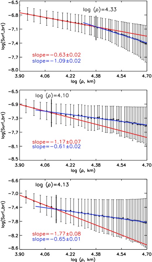
The ‘log–log’ dependence of the azimuthally averaged surface brightness on the projected distance for the coadded R-images obtained on 12 Sept. 2016 (the top panel); on 2016 Sept. 22 (the middle panel); and on 2016 Oct. 4 (the bottom panel). The lines indicate the distance, where the profile slopes change.

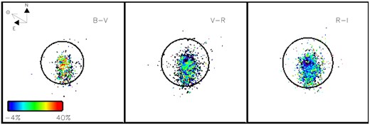
The colour maps constructed from the coadded images obtained on 2016 Sept. 12. Circles mark the outer apertures containing the colour image of the coma: 50 pxl (or about 49 000 km), 52 pxl (or about 51 300 km), and 62 pxl (or about 62 000 km) in the right-hand, middle, and left-hand panels, respectively.
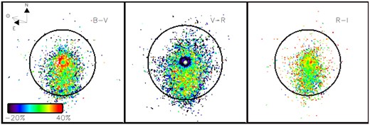
The colour maps constructed from the coadded images obtained on 2016 Sept. 22. Circles mark the outer apertures containing the colour image of the coma: 36 pxl (or about 35,000 km), 40 pxl (or about 39,000 km), and 42 pxl (or about 41,000 km) in the right, middle, and left panels, respectively.
The colour maps constructed from the coadded images obtained on 2016 Oct. 4. Circles mark the outer apertures containing the colour image of the coma: 50 pxl (or about 49 000 km) in the left-hand and middle panels, and 62 pxl (or about 60 000 km) in the right panel.
Given that the colour image of the coma has more symmetric appearance for the observing night of September 12, we calculated the radial dependence of the coma reddening by averaging the colour values within concentric annuli of increasing radii. The radial dependence of the reddening is depicted in Fig. 14 for the B-V, V-R, and R-I spectral intervals. We observe that the reddening of the coma measured from the images taken on September 12 is positive – the coma colour is redder than the colour of the Sun. The slope of the spectral continuum is higher in the B-V spectral interval within distances of approximately 34 000 km from the nucleus; at larger distances the slope changes, becoming higher in the R-I spectral domain. The continuum slope in the B-V band decreases gradually from the inner to outer part of the coma. The change in the reddening profile is also seen in the V-R spectral interval. For the data obtained during the two other runs, the images of Echeclus’ coma is highly asymmetric due to the jet-like feature directed to the south. Therefore, we calculated the radial dependence of the reddening by averaging the signal in the narrow segment of position angles, between 179° and 220°. These reddening profiles are presented in Fig. 15 for three observing epochs.
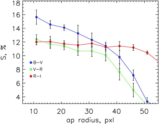
The reddening profiles calculated from concentric annuli versus annulus radius for the data obtained on 2016 September 12.
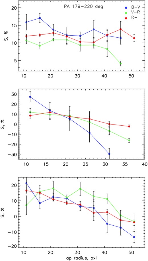
The reddening profiles calculated for the position angle segment 179°– 220°for the data obtained on September 12 (top), September 22 (middle), and October 4 (bottom).
It can be noted that the coma is somewhat shrunk on 2016 September 22 (see Fig. 12); the reddening of the south region of the coma became negative in the B-V and V-R spectral intervals at about 25 pxl from the optocenter, which corresponds to approximately 24 500 km. The B-V reddening profile calculated from the images taken on October 4 turns to negative values at somewhat larger distances from the optocentre (35–40 pxl or about 34 000–39 000 km). The decrease in the reddening with increasing distance from the optocentre can be noted for three observing nights, furthermore, the effect is less pronounced in the R-I spectral interval. It is interesting to note that the innermost part of the coma (a ring around the central pixels) was observed considerably bluer in the V-R spectral region during the night October 4. In order to confirm reality of this feature we checked out each individual image from which the V and R – composite images are comprised. The accuracy of the Echeclus’ magnitudes calculated from the individual images is about 0.01 mag pointing out the stable photometric condition during the night. Also as it was noted above, the two sets of standards used for the absolute photometric calibration (the Stetson fields and the field SDSS stars) give the satisfactory agreement of the transformation coefficients. And, finally, the centres of the shifted images, which were coadded to form the composite V and R–images for the colour calculation, have a scatter around their mean values at a level of 0.1 pxl.
In order to inspect the colour of the Echeclus’ image obtained on October 4 more carefully we calculated the reflectivity gradient using the difference between the coma surface brightness (in mag/arcsec2) measured in the different colour bands. The magnitudes were azimuthally averaged within the narrow annuli ranging from 2 to 20 pxl (or 1900–19 500 km of the projected distance). The magnitude differences B − V, V − R, R − I were used to calculate reflectivity gradient. The result is depicted in Fig. 16 for the B − V, V − R, and R − I spectral intervals. The steep decrease in the coma colour is observed in the V − R spectral interval within 6 pxl from the photocentre, the same decrease in the colour we can see as a ring feature in the middle panel of Fig. 13. The pronounce difference in the colour is observed between the very red central part of the image and bluer ambient coma region. This colour change is in agreement with the result reported by Seccull et al. (2019), who found that the Echeclus’ nucleus is redder than the surrounding coma region.
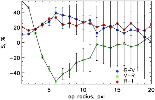
The reddening profiles calculated from the inner part of the Echeclus’ images (between 2 and 20 pxl) obtained on Oct. 4.
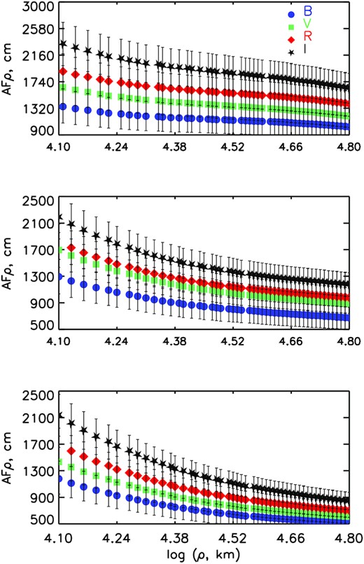
The Afρ parameter calculated for the B,V,R,I filters versus aperture radii projected at the Echeclus distance. From top to bottom results corresponding to Sept. 12, Sept. 22 and Oct. 4.
In Table 4 we present a summary of the photometric parameters, which were calculated using the integrated signal in aperture of 2.5 arcsec corresponding to projected distance of 10 000 km to facilitate comparison with results obtained from other observing epochs by other teams as well as the Afρ parameters extracted with larger aperture of about 6 arcsec (or about 23 400 km). Since the observations were performed at different phase angles, we corrected magnitudes and Afρ parameters for a 0° phase angle to take into account an opposition effect with a linear coefficient of 0.02 mag.deg−1 (Meech & Jewitt 1987). The Afρ parameters measured with aperture 2.5 arcsec do not change from night to night, likely, due to contribution the nucleus flux to the coma. Meanwhile the Afρ measured with larger aperture demonstrates a decline in Echeclus’ activity.
Photometric parameters extracted from aperture of 2.5 arcsec, as well as Afρ parameter from aperture of about 6 arcsec. The magnitudes and Afρ are corrected to 0° phase angle.
| Date | filter | mag | Afρ,cm | Afρ,cm | S, %/1000 Å |
|---|---|---|---|---|---|
| ρ = 2.5 arcsec | ρ = 6.2 arcsec | ρ = 2.5 arcsec | |||
| 2016 September 12 | B | 18.34 ± 0.02 | 1640 ± 110 | 1280 ± 80 | 17.6 ± 2.0, (B-V) |
| V | 17.51 ± 0.01 | 2020 ± 100 | 1540 ± 80 | 15.6 ± 1.3, (V-R) | |
| R | 16.97 ± 0.01 | 2340 ± 120 | 1770 ± 90 | 15.1 ± 0.9, (R-I) | |
| I | 16.46 ± 0.01 | 2900 ± 150 | 2150 ± 100 | – | |
| 2016 September 22 | B | 18.31 ± 0.02 | 1670 ± 100 | 950 ± 80 | 20.4 ± 1.7, (B-V) |
| V | 17.45 ± 0.01 | 2100 ± 100 | 1210 ± 60 | 10.1 ± 1.4, (V-R) | |
| R | 16.97 ± 0.01 | 2330 ± 120 | 1340 ± 70 | 13.4 ± 1.0, (R-I) | |
| I | 16.48 ± 0.01 | 2820 ± 140 | 1620 ± 80 | – | |
| 2016 October 4 | B | 18.44 ± 0.02 | 1490 ± 100 | 770 ± 60 | 16.5 ± 0.5, (B-V) |
| V | 17.63 ± 0.01 | 1800 ± 90 | 930 ± 50 | 18.6 ± 0.9, (V-R) | |
| R | 17.05 ± 0.01 | 2160 ± 110 | 1090 ± 60 | 16.4 ± 0.5, (R-I) | |
| I | 16.53 ± 0.01 | 2700 ± 140 | 1360 ± 70 | – |
5 ORBITAL EVOLUTION
The orbital history of Echeclus has recently been investigated by Kareta et al. (2019). This study emphasized, in simulating the orbits of 100 clones, that our knowledge of the orbit of Echeclus could be described only by statistics over more than 1000 yr forward and backward in time. This is due to the fact that Echeclus is subjected to close encounters with Jupiter and Saturn, and the past-close encounters orbit is very sensitive to the initial conditions, i.e. the geometrical configuration of the close encounter. This is why close encounters tend to disperse clouds of clones.
We here revisit that study, taking advantage of updated ephemeris of Echeclus.
5.1 Two critical close encounters with Jupiter
We simulated the orbits of 1000 clones of Echeclus, using four independent dynamical models:
Model 1: we simulate the orbit of Echeclus perturbed by the eight planets. For this, we integrate numerically the equations of motion of Echeclus in heliocentric Cartesian coordinates with the Adams-Bashforth-Moulton 10th-order predictor-corrector integrator (Hairer, Nørsett & Wanner 1993). We neglect general relativity and the mass of Echeclus when simulating its positions, however the positions of the eight planets are given by the orbital theory INPOP19a, in which additional effects like the general relativity and the masses of large asteroids are included (Fienga et al. 2019). These ephemerides are valid over the period ranging from 1000 to 3000. We limit our study to this time range.
Model 2 uses JPL DE 422 ephemerides instead of INPOP19a. The JPL Horizon server provides different planetary ephemerides, we used DE 422 because its interval of validity is close to our interval of study. DE 431 is more recent, but provides positions over ≈30,000 yr, which is likely to result in a degradation of the accuracy to reduce the size of the provided binary file.
Model 3 uses JPL DE 431, and is suitable for longer term studies (Section 5.2)
Model 4: based on a simulation of Echeclus’ orbit perturbed by the eight planets, this time using the existing software package REBOUND, specifically for its high order integrator IAS15. The ephemerides are taken from the JPL Horizons server using an automated function that downloads the most up-to-date data on each of the bodies. In this case, it uses identical ephemerides to our Model 3, JPL DE 431. The positions of the planets and each individual Echeclus clone are calculated at each time-step. The clones are seen as independent test particles and do not interact with each other.
These four models included the planetary ephemeris thanks to the CALCEPH library (Gastineau et al. 2015). The initial position and velocity of Echeclus (cf. Table 5) are taken from JPL Horizons in the ecliptic reference frame at the epoch JD 2458849.5, which corresponds to 2020 January 1 at 00h00m00s TDB.
Our initial conditions of Echeclus at the Epoch JD 2458849.5, with respect to the ecliptic plane.
| x | 2.014404165731244 au |
| y | 9.051805601802508 au |
| z | −0.7006284623276615 au |
| |$\dot{x}$| | −4.680331663606411 × 10⁻³ au/d |
| |$\dot{y}$| | 3.743918693058765 × 10⁻³ au/d |
| |$\dot{z}$| | −2.407860303817577 × 10⁻⁴ au/d |
| x | 2.014404165731244 au |
| y | 9.051805601802508 au |
| z | −0.7006284623276615 au |
| |$\dot{x}$| | −4.680331663606411 × 10⁻³ au/d |
| |$\dot{y}$| | 3.743918693058765 × 10⁻³ au/d |
| |$\dot{z}$| | −2.407860303817577 × 10⁻⁴ au/d |
The clones are generated from the covariance matrix provided by the JPL Small-Body Browser (equation A1). We generated the clones first by running a Cholesky decomposition of the covariance matrix, and from it a multivariate Gaussian distribution of the orbital elements, in using the GNU Scientific Library (e.g. Galassi et al. 2006), version 2.6. The orbital elements are finally converted into heliocentric Cartesian coordinates.
The orbital elements of our simulated clones are shown in Fig. 18. In this Figure, we can see that all the clones present roughly the same dynamics over the period ≈1200 CE to ≈2900 CE, while they disperse beyond these points. The dispersal of the clones occur in 1179 and 2887, and correspond to close encounters with Jupiter (Table 6).
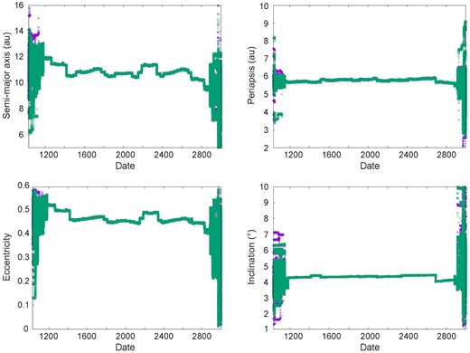
Orbital elements of our 1000 clones of Echeclus in the Models 1 and 2.
The close encounters between Jupiter and Echeclus, which spread the clones.
| Date | Distance | Date | Distance | |
|---|---|---|---|---|
| Model 1 (INPOP19a) | 1179.90 | 0.933 au | 2887.22 | 1.37 au |
| Model 2 (DE 422) | 1179.90 | 0.929 au | 2887.09 | 1.49 au |
| Date | Distance | Date | Distance | |
|---|---|---|---|---|
| Model 1 (INPOP19a) | 1179.90 | 0.933 au | 2887.22 | 1.37 au |
| Model 2 (DE 422) | 1179.90 | 0.929 au | 2887.09 | 1.49 au |
Model 3, which we suspect to be less accurate given its range of validity, diverges from the other models at the dates 1262.50 and 2341.50. These dates correspond to close encounters with Jupiter in all the models, but at different distances. DE 431 based models estimate them at 1.320 au and 1.706 au, respectively, while INPOP19a and DE422 based models predict 2.160 au and 1.950 au, respectively. Regardless, we continue to use it to study the orbital dynamics of Echeclus over the period 12 000 BCE to 16 000 CE, to investigate whether its activity could be related to its past orbit.
The same process was applied with Model 4 using REBOUND. While the clones also diverge after the same close encounters with Jupiter, the minimum distance is slightly different while still within the estimates calculated by the other models. The close encounter in 1262.50 brings the clones to 2.135 au from Jupiter and the one in 2341.50 to 1.702 au. Beyond these close encounters, the clones are so scattered that any estimate of Echeclus’ trajectory remains uncertain.
Kareta et al. (2019) simulated the evolution of 100 clones of Echeclus with REBOUND. They found that the trajectories diverged at 1144 CE and 2970 CE, these dates corresponding to close approaches to Jupiter at 0.90 and 1.98 au, respectively. These significant differences with the close encounters we detect in Table 6 are probably due to an update of the JPL ephemeris since that previous study, and the differences due to the models themselves. In particular, using orbital ephemeris like we do in the models 1 to 3 guarantees a very high accuracy on the location of the planets at any time, provided this accuracy is not hampered by the numerical sampling of the provided ephemeris.
5.2 Orbital dispersion
This last formula must be normalized to be interpreted as a probability density function, i.e. divided by 500. In practice A should be smaller than 500 since a few clones are ejected from the Solar System (which means, for backward integration, that they would be interstellar visitors). The parameters are fitted with the non linear trust region method provided by the Gnu Scientific Library, and the outcomes are given in Tables A2 to A5, while the resulting statistics are plotted in Fig. 19.
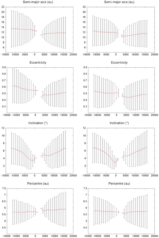
Statistical distribution of the orbital elements of Echeclus, simulated with the Model 3 (left), and REBOUND (right). The error bars represent ±σ.
These results essentially illustrate that we cannot give reliable predictions on the past and future of Echeclus. Only the pericentric distance remains constrained. This is likely due to the dynamical complexity of the region of the Centaurs (e.g. Fernández, Helal & Gallardo 2018). One of the conclusions of this paper is that active Centaurs often – but not always– have had recent drops in perihelia. Our dynamical study concludes that in was not the case for Echeclus.
We also attempted to fit a Rice distribution to the orbital elements, as in (e.g. Laskar 2008). The fit was at best as efficient as the Gaussian distribution for the semi-major axis and the pericentric distance, while it did not converge for the inclination.
6 DISCUSSION
The new observational data and data analysis presented in this paper bring new information about the physical properties of Echeclus. The main result concerns the shape model and the pole orientation, which are now significantly constrained. The results provided by this study are in good agreement with previous work based on the modelling of the main outburst observed in 2005 (Rousselot et al. 2016), i.e. that the obliquity of the pole orientation is extremely high, the rotational axis being probably nearly parallel to the ecliptic (obliquity superior to ∼50°, as shown Fig. 7). The shape model also shows that Echeclus is also significantly elongated, with a semi-major axial ratio a/b = 1.32 (and b/c ∼ 1.1 but this second ratio is poorly constrained by our photometric data).
These two parameters imply a strong seasonal effect on Echeclus during its orbital motion, some regions being exposed for only a fraction of its orbit. The geometry of the pole orientation with respect to its position along the orbit and during the different outbursts reveals that different regions of the nucleus contribute to the different outbursts. This was already pointed out by the modelling of the main outburst (Rousselot et al. 2016), which could satisfactorily be explained by three different sources located on both hemispheres (as well as by an important obliquity for its polar orientation). It should be stressed, nevertheless, that more complicated shapes, such as bimodal structures similar to 486958 Arrokoth or to comet 67P/Churyumov-Gerasimenko, cannot be excluded. In such a case seasonal effects would presumably be more important.
Our detailed study of the dust colour and cometary activity observed during the 2016 outburst reveals the presence of several jets around the nucleus during the outburst, the main one appearing in the southward direction. The colour properties of the dust appears to change with cometocentric distance: the normalized reflectivity decreases with increasing cometocentric distance. This normalized reflectivity remains positive in the coma images obtained on October 12, which is indicative of a coma reddening. For the September 22 and October 4 data the negative gradient of the normalized reflectivity characterizes the coma at large cometocentric distances in the jet vicinity. Such variations in the dust colour properties can be indicative of changes in grain size or in composition. These results are in qualitative agreement with those published by Seccull et al. (2019) (same outburst) and Kareta et al. (2019) (2017 outburst), based on spectroscopic data. The observational data published by Seccull et al. (2019), obtained 3 days after our images, on 2016 October 7, would indicate a bluer dust (negative slope in the normalized reflectance spectrum, computed between the near-infrared and the optical range) and considerable difference in the colour between nucleus and ambient coma. The images obtained on October 4 confirm this trend in the V − R spectral interval. Seccull et al. (2019) suggest that this colour difference could be explained by the two particle population with different optical properties. Alternative explanation was proposed by Zubko, Videen & Kulyk (2020) who stress that the different scattering regimes [i.e. the single-particle scattering in the optically thin coma against multiply scattering from the regolith surface) could lead to the change in reflectivity slope. The data published by Kareta et al. (2019) remains positive in the slope but bluer than Echeclus itself (two different slopes are computed, a first one with an aperture of 1 arcsec (Echeclus alone) and another one with an aperture of 2.2 arcsec (Echeclus plus the inner coma)]. Our colour maps and reddening profiles confirm the trend of changing in the colour with cometocentric distance.
The study of Echeclus orbital evolution shows that its perihelion distance has probably remained larger than 4 au over the past 12 000 yr, at least. Such a relatively large perihelion distance, compared to the one of ‘usual’ comets, makes a water ice sublimation powered activity unlikely for Echeclus. Its present activity being mainly characterized by random and strong outbursts separated by long periods (several yr) without activity or a very weak one (unlike a Centaur like 29P/Schwassmann-Wachmann with a more regular activity). Even if close encounters with giant planets in the past prevents any firm conclusion for orbital characteristics of Echeclus for periods larger than 12 000 yr it seems that the material now ejected during outburst comes from areas in the nucleus containing rather ‘fresh’ material, that have not suffered a long period of important cometary activity. In any case our dynamical study shows that Echeclus did not suffered any significant change to its orbital elements (mainly the perihelion distance) since, at least, ≈1200 CE.
The lifetime of currently observed outbursts is also difficult to predict. A rough estimate of the mass loss during each event, compared to its orbital period, lead to a negligible mass loss, even for periods of millions of yr. Indeed, with some events lasting a few hours and even with an upper limit of about 400 kg.s−1 (Wong, Mishra & Brown 2019), i.e. a mass loss inferior to about 107 kg / outburst (case of the 2005 outburst, the more important one), this would lead to a mass loss rate, with the present orbital period and 5 outburst / orbit, to about 0.003 per cent of mass loss per million yr (assuming a bulk density of 1000 kg.m−3 and the diameter above mentioned). Such a long lifetime for its present activity does not provide any constraint for the duration of this process. It is rather the long term instability of Echeclus’ orbit, that probably comes from larger heliocentric distances – like the Centaur population – that is indicative of a recent physical process, at the timescale of Solar system history.
7 CONCLUSION
This paper presents new observational data and a data analysis that bring important constraints to Echeclus physical properties. The main results are:
A shape model that shows a high obliquity of the rotational axis (larger than about 50°). Our model also shows that Echeclus, which is a small Centaur, is also significantly elongated with a semi-major axial ratio a/b = 1.32 (and b/c ∼ 1.1 but this second ratio being poorly constrained by our photometric data). Such constraints highlight the probable importance of seasonal effects on Echeclus’ recurrent outbursts. The computed sidereal rotation period is P = 26.785178 ± 10−6 h.
Our study of the dust properties during the 2016 outburst shows significant changes in the colour with the cometocentric distance. The larger the cometocentric distance, the bluer is the dust colour. The reddening profile in the inner coma shows a ring-like structure for the images obtained on October 4 with a bluer dust computed with the V-R colour index. A main jet is also apparent in the southward orientation. We provide measurements of the Afρ parameter that is as high as ≈2600 cm extracted with projected aperture of ≈10 000 km for the images obtained in the I filter.
Our study of the orbital history of Echeclus’ orbital evolution highlight the importance of close encounters with giant planets that implies an unstable orbit for Echeclus at large timescale (more than a few 10 000 yr). For a period of 12 000 yr the main conclusion is that Echeclus perihelion distance was greater than about 4 au, preventing it to follow a typical cometary activity like a short-period comet.
In any case Echeclus deserves to be carefully monitored to gather more information about its next outbursts and to cover, at least, a complete orbital period. Such intensity in cometary ourburst for a small body orbiting as far from the Sun is unique and can lead to a better understanding of cometary activity not driven by water sublimation.
ACKNOWLEDGEMENTS
Based on observations made with European Southern Observatory (ESO) Telescopes at the La Silla Paranal Observatory under program 297.C-5060.
This project has received funding from the European Union’s Horizon 2020 research and innovation programme under grant agreement No 730890. This material reflects only the authors views and the commission is not liable for any use that may be made of the information contained therein.
We also acknowledge the use of Starlink software which is currently supported by the East Asian Observatory.
DATA AVAILABILITY
Data available on request.
Footnotes
cf JPL Small-Body Database Browser https://ssd.jpl.nasa.gov/sbdb.cgi
REFERENCES
APPENDIX A: ORBITAL DISPERSION
The correlation matrix we used to generate our 1000 clones (from the JPL Small-Body Browser). The 6 columns being the eccentricity e, the perihelion q (au), the time of perihelion passage tp (days), the longitude of the ascending node Ω, the argument of the perihelion ω, and the ecliptic inclination i. These angles are expressed in degrees.
 |
|
The correlation matrix we used to generate our 1000 clones (from the JPL Small-Body Browser). The 6 columns being the eccentricity e, the perihelion q (au), the time of perihelion passage tp (days), the longitude of the ascending node Ω, the argument of the perihelion ω, and the ecliptic inclination i. These angles are expressed in degrees.
|
|
Fit of a Gaussian distribution on the semi-major axis of 1000 clones. For each date, the first line results from the Model 3, while the second one results from the Model 4. See Section 5.2 for more details.
| Date | A | μ | σ |
|---|---|---|---|
| −12 000 | 443.60 ± 0.41 | 13.279 ± 0.017 | 7.263 ± 0.023 |
| −12 000 | 453.22 ± 0.54 | 12.503 ± 0.022 | 6.045 ± 0.029 |
| −7000 | 474.20 ± 0.25 | 13.153 ± 0.009 | 6.353 ± 0.013 |
| −7000 | 472.82 ± 0.39 | 12.077 ± 0.014 | 5.246 ± 0.019 |
| −1000 | 494.41 ± 0.11 | 12.808 ± 0.003 | 3.078 ± 0.004 |
| −1000 | 496.99 ± 0.09 | 11.898 ± 0.002 | 3.365 ± 0.003 |
| 5000 | 498.07 ± 0.14 | 11.313 ± 0.003 | 2.289 ± 0.005 |
| 5000 | 496.91 ± 0.13 | 10.492 ± 0.004 | 3.235 ± 0.005 |
| 10 000 | 482.98 ± 0.26 | 11.576 ± 0.009 | 4.914 ± 0.013 |
| 10 000 | 473.78 ± 0.38 | 11.045 ± 0.014 | 4.712 ± 0.019 |
| 16 000 | 463.82 ± 0.32 | 11.781 ± 0.013 | 6.184 ± 0.017 |
| 16 000 | 447.16 ± 0.41 | 11.433 ± 0.016 | 5.364 ± 0.022 |
Fit of a Gaussian distribution on the eccentricity of 1000 clones.For each date, the first line results from the Model 3, while the second one results from the Model 4.
| Date | A | μ | σ |
|---|---|---|---|
| −12 000 | 540.69 ± 1.53 | 0.6211 ± 0.0012 | 0.2657 ± 0.0011 |
| −12 000 | 528.91 ± 1.07 | 0.5408 ± 0.0009 | 0.2549 ± 0.0010 |
| −7000 | 524.52 ± 1.76 | 0.5747 ± 0.0014 | 0.2272 ± 0.0015 |
| −7000 | 520.58 ± 0.86 | 0.5094 ± 0.0007 | 0.2272 ± 0.0009 |
| −1000 | 500.51 ± 0.65 | 0.5461 ± 0.0004 | 0.1006 ± 0.0006 |
| −1000 | 509.59 ± 1.05 | 0.5078 ± 0.0008 | 0.14218 ± 0.0011 |
| 5000 | 501.53 ± 0.47 | 0.4782 ± 0.0003 | 0.1007 ± 0.0004 |
| 5000 | 508.91 ± 0.69 | 0.4434 ± 0.0006 | 0.1684 ± 0.0008 |
| 10 000 | 490.33 ± 0.48 | 0.4839 ± 0.0004 | 0.1894 ± 0.0005 |
| 10 000 | 506.20 ± 0.42 | 0.4595 ± 0.0004 | 0.2182 ± 0.0005 |
| 16 000 | 480.15 ± 0.42 | 0.5151 ± 0.0004 | 0.2229 ± 0.0004 |
| 16 000 | 501.09 ± 0.79 | 0.4865 ± 0.0007 | 0.2378 ± 0.0008 |
Fit of a Gaussian distribution on the inclination of 1000 clones. For each date, the first line results from the Model 3, while the second one results from the Model 4.
| Date | A | μ | σ |
|---|---|---|---|
| −12 000 | 493.38 ± 0.15 | 6.6523 ± 0.0162 | 4.1727 ± 0.0238 |
| −12 000 | 499.18 ± 0.09 | 6.7180 ± 0.0091 | 3.9060 ± 0.0132 |
| −7000 | 494.69 ± 0.14 | 5.7294 ± 0.0138 | 3.6242 ± 0.0202 |
| −7000 | 499.27 ± 0.09 | 5.9077 ± 0.0082 | 3.3131 ± 0.0119 |
| −1000 | 498.92 ± 0.08 | 3.3607 ± 0.0054 | 1.6374 ± 0.0077 |
| −1000 | 499.19 ± 0.10 | 2.9594 ± 0.0068 | 1.8200 ± 0.0100 |
| 5000 | 499.24 ± 0.06 | 4.9033 ± 0.0039 | 1.5070 ± 0.0056 |
| 5000 | 499.28 ± 0.06 | 4.5889 ± 0.0049 | 2.0106 ± 0.0069 |
| 10 000 | 494.53 ± 0.14 | 5.2405 ± 0.0140 | 3.8301 ± 0.0211 |
| 10 000 | 499.41 ± 0.09 | 5.6027 ± 0.0095 | 3.7978 ± 0.0141 |
| 16 000 | 486.72 ± 0.16 | 6.6608 ± 0.0181 | 4.6051 ± 0.0270 |
| 16 000 | 499.14 ± 0.09 | 7.0315 ± 0.0096 | 4.2971 ± 0.0140 |
Fit of a Gaussian distribution on the pericentric distance of 1000 clones. For each date, the first line results from the Model 3, while the second one results from the Model 4.
| Date | A | μ | σ |
|---|---|---|---|
| −12 000 | 498.74 ± 0.23 | 5.6549 ± 0.0045 | 0.9567 ± 0.0064 |
| −12 000 | 498.79 ± 0.19 | 5.7742 ± 0.0041 | 1.1023 ± 0.0059 |
| −7000 | 499.14 ± 0.21 | 5.6872 ± 0.0037 | 0.7766 ± 0.0052 |
| −7000 | 498.73 ± 0.18 | 5.7363 ± 0.0036 | 0.9097 ± 0.0050 |
| −1000 | 499.48 ± 0.10 | 5.7189 ± 0.0012 | 0.3774 ± 0.0018 |
| −1000 | 499.69 ± 0.14 | 5.7063 ± 0.0018 | 0.3833 ± 0.0026 |
| 5000 | 499.54 ± 0.08 | 5.7866 ± 0.0010 | 0.43544 ± 0.0015 |
| 5000 | 499.24 ± 0.17 | 5.6122 ± 0.0026 | 0.5538 ± 0.0037 |
| 10 000 | 499.03 ± 0.18 | 5.8545 ± 0.0037 | 1.0066 ± 0.0052 |
| 10 000 | 498.81 ± 0.21 | 5.7229 ± 0.0044 | 1.0375 ± 0.0063 |
| 16 000 | 492.43 ± 0.23 | 5.9242 ± 0.0054 | 1.3068 ± 0.0076 |
| 16 000 | 498.48 ± 0.25 | 5.7338 ± 0.0058 | 1.3018 ± 0.0081 |
