


ABSTRACT
We study magnetohydrodynamic stability of neutron star core matter composed of neutrons, protons, and leptons threaded by a magnetar-strength magnetic field 1014–1017 G, where quantum electrodynamical effects and Landau quantization of fermions are important. Stability is determined using the Friedman–Schutz formalism for the canonical energy of fluid perturbations, which we calculate for a magnetizable fluid with H ≠ B. Using this and the Euler–Heisenberg–Fermi–Dirac Lagrangian for a strongly magnetized fluid of Landau-quantized charged fermions, we calculate the local stability criteria for a neutron star core with a spherical axisymmetric geometry threaded by a toroidal field, accounting for magnetic and composition gradient buoyancy. We find that, for sufficiently strong fields B ≳ 1015 G, the magnetized fluid is unstable to a magnetosonic-type instability with growth times of the order of 10−3 s. The instability is triggered by sharp changes in the second-order field derivative of the Euler–Heisenberg–Fermi–Dirac Lagrangian that occur where additional Landau levels start being populated. These sharp changes are divergent at zero temperature, but are finite for non-zero temperature, so realistic neutron star core temperatures 5 × 10⁷ K < T < 5 × 10⁸ K are used. We conjecture that this mechanism could promote the formation of magnetic domains as predicted by Blandford and Hernquist and Suh and Mathews.
1 INTRODUCTION
The problem of magnetohydrodynamic (MHD) stability is of great importance to the study of magnetars and compact stars in general, since their magnetic field configurations must be stable over time-scales much longer than their dynamical time-scales. Determining which types of field configuration are allowed by stability considerations is of particular interest following the discovery of a multipolar field configuration in a neutron star by the NICER experiment (Bilous et al. 2019; Riley et al. 2019); the dipolar field model often assumed is clearly too simple. Understanding the field configuration of magnetars and how they could be destabilized is also of fundamental interest in helping to understand their emission mechanisms, including the theoretical explanation for soft gamma repeaters as caused by fractures in the magnetar crust (Thompson & Duncan 1995; Heyl & Hernquist 2005) or field reconnection in the magnetosphere (Lyutikov 2006). Magnetars are also a leading candidate for the source of fast radio bursts (FRBs; Popov & Postnov 2010; Lyubarsky 2014, 2020; Beloborodov 2017; Lu & Kumar 2018; Metzger, Margalit & Sironi 2019), and a recent detection by the CHIME radio telescope of an FRB originating from a magnetar in our Galaxy (CHIME/FRB Collaboration 2020) has provided evidence that this could be the case. MHD instabilities within the star could power magnetic outbursts that deposit energy into the magnetar magnetosphere, which in turn powers the different proposed FRB mechanisms.
Though the complicated nature of MHD has made aspects of MHD stability intractable to analytical study, many useful results have been proven analytically and later confirmed numerically for the stability of stellar magnetic fields. A purely toroidal stellar field is known to be unstable along the axis of symmetry to sausage (e.g. interchange) and kink instabilities (Tayler 1973), while a purely poloidal field with closed field lines within the star is also unstable to sausage and kink instabilities where the field vanishes (Markey & Tayler 1973; Wright 1973). Flowers & Ruderman (1977) showed that a star with a purely poloidal field is unstable even if no field lines are closed within it. Markey & Tayler (1973) and Wright (1973) both suggested that a mixed poloidal–toroidal field configuration could be stable, which was demonstrated numerically (Braithwaite & Spruit 2004; Braithwaite & Nordlund 2006; Yoshida, Yoshida & Eriguchi 2006; Duez, Braithwaite & Mathis 2010) for near equal-strength poloidal and toroidal fields. Simulations by Braithwaite (2009) showed that mixed toroidal–poloidal configurations can be stable with a much weaker poloidal component, which was confirmed analytically by Akgün et al. (2013). Stable stratification of a star, represented mathematically by a positive square Brunt–Väisälä frequency, has been shown analytically (Tayler 1973) and numerically (Braithwaite & Nordlund 2006) to stabilize the magnetic field, and in general it allows for a greater variety of possible field configurations since the field no longer needs to be a solution of the Grad–Shafranov equation (Reisenegger 2009). Using numerical simulations, Mitchell et al. (2015) found that different field configurations in barotropic stars always decayed away, giving further evidence to the idea that stable stratification must be included to obtain a stable field configuration. Stable stratification alone may not be sufficient to stabilize a fluid with a magnetic field that diminishes quickly enough with increasing height, which can be unstable to magnetic buoyancy (Parker 1955; Acheson 1979). Additionally, as discussed by Reisenegger (2009), the erosion of stable stratification by dissipative processes (weak decays and ambipolar diffusion in neutron stars) could lead to field rearrangement and perhaps instability.
Previous analyses of the stability of stellar magnetic fields have made the often reasonable assumption that the stellar medium through which the field is threaded is not magnetizable i.e. that B = H. This is clearly not the case for superfluid-superconducting neutron stars, nor is it true for extremely strong magnetic fields. The field strengths attained in magnetars are up to 1015 G at the surface and perhaps one to two orders of magnitude greater in the core (Mereghetti, Pons & Melatos 2015; Turolla, Zane & Watts 2015; Kaspi & Beloborodov 2017; Uryu et al. 2019). Since these fields exceed the quantum critical field |$B_{\text{crit}}=m_{\text{e}}^2/e=4.4\times 10^{13}$| G, quantum electrodynamic effects are relevant and could be important to magnetar stability. In the vacuum case, non-linear electromagnetic effects are encoded in the Euler–Heisenberg Lagrangian (Heisenberg & Euler 1936). In matter, this must be supplemented with terms accounting for the interaction of fermions with the magnetic field. These additional Lagrangian terms have been computed for a charged Fermi gas at zero temperature T (Chodos, Everding & Owen 1990) and at finite T (Elmfors, Persson & Skagerstam 1993; Persson & Zeitlin 1995). In the presence of such strong fields, the charged fermions in a neutron star will undergo Landau quantization, which modifies the equation of state (EOS; Lai & Shapiro 1991; Broderick, Prakash & Lattimer 2000; Mao, Iwamoto & Li 2003; Chamel et al. 2012; Sinha, Mukhopadhyay & Sedrakian 2013; Chamel & Stoyanov 2020), magnetization, and transport properties (Potekhin 1999; Potekhin & Yakovlev 2001; Potekhin, Pons & Page 2015) of the star. The effects of B ≲ 1018 G on the EOS are generally quite small at typical core densities, and B ≈ H to within a few per cent. However, the analysis of MHD stability requires not only examining the first-order partial derivatives of the magnetic free energy, but its second-order derivatives with respect to B and the density ρ. These derivatives have been studied in the context of magnetic domain formation in strong fields by Blandford & Hernquist (1982) and Suh & Mathews (2010), but as far as the authors are aware, the implications of strong-field quantum mechanical effects on MHD stability have not been examined in the literature.
In this paper, we study MHD stability including non-linear, non-vacuum electromagnetism appropriate for magnetar-strength magnetic fields. We employ the canonical energy approach to stability analysis (Bernstein et al. 1958) and in particular follow closely the coordinate basis version of the non-relativistic fluid perturbation theory expounded by Friedman & Schutz (1978). We extend the non-relativistic MHD perturbation theory of Glampedakis & Andersson (2007) to B ≠ H to allow us to consider the effect of the medium and vacuum magnetization on MHD stability. We also consider non-barotropic EOS, and employ a Brunt–Väisälä frequency accounting for both neutron–proton fraction buoyancy (Reisenegger & Goldreich 1992) and leptonic buoyancy (Kantor & Gusakov 2014; Passamonti, Andersson & Ho 2016; Yu & Weinberg 2017; Rau & Wasserman 2018), in contrast to e.g. Akgün et al. (2013), who only included the neutron–proton fraction buoyancy in their analysis and were considering the global instability of specific axisymmetric fields. We consider the local stability of strongly magnetized neutron star core fluid in a planar geometry, in which the effects on stability of non-linear electromagnetism and an accurate buoyant force, including magnetic buoyancy, are more easily understood than in the spheroidal star case. After reviewing the electromagnetic Lagrangian and the relevant partial derivatives of it which determine the stability, we conclude by discussing its numerical application to the stability criterion for the planar fluid case. The background magnetic field in the neutron star crust obeys a fundamentally different constraint equation compared to ideal MHD (Cumming, Arras & Zweibel 2004; Gourgouliatos et al. 2013), and the stability analysis is fundamentally different (Lyutikov 2013); we thus leave this subject to a subsequent paper.
In Section 2, we introduce the canonical energy for B ≠ H MHD, with most details of the derivation left to the supplemental Appendix A. Section 3 derives the stability criteria using the canonical energy. In Section 4, the pressure and energy density for strong fields and Landau quantized fermions are discussed in detail and the required thermodynamic derivatives are derived, and the background stellar model is described. Section 5 describes the numerical results for the stability criteria, and Section 6 discusses their observational implications. The supplemental Appendix B gives explicit expressions for thermodynamic partial derivatives used in evaluating the stability criteria. We work in Gaussian units and set c = ℏ = 1. We also employ the Einstein summation convention using Latin letters as spatial indices i = 1, 2, 3. The letter a is reserved as a subscript to denote particle species a = n, p, e, m, with sums over particle species always denoted explicitly.
2 MHD EQUATIONS AND CANONICAL ENERGY
We consider a non-rotating neutron star core composed of neutrons n, protons p, electrons e and, at sufficiently high densities, muons m. We assume the magnetic field is strong enough to destroy proton superconductivity, and ignore neutron superfluidity. We also assume that the collisional coupling time between the fluids is short and that they all comove – this would not be the case if the neutrons were a superfluid, but the charged fluids are expected to comove generally. We work in the ideal MHD approximation of zero net electric charge density ρe = 0 and infinite conductivity.
For simplicity, we have assumed zero temperature, and hence zero entropy, in the equations of motion. The T = 0 limit is a very good approximation for the neutron star core where the fermion chemical potentials μa satisfy μa ≫ kBT. An exception is made for certain second-order partial derivatives of umat, which we discuss in Section 4. In these terms, we treat the temperature as a fixed parameter and do not concern ourselves with the dynamics of the entropy.
We now derive the canonical energy for a magnetizable fluid, which is used to study the fluid’s MHD stability. We follow the definitions of the Lagrangian perturbations of fluid quantities of Friedman & Schutz (1978), which has antecedents in Taub (1969), Carter (1973), Friedman & Schutz (1975), and Bardeen et al. (1977), and which has been applied to MHD by Glampedakis & Andersson (2007). In these definitions, we work in a coordinate basis and hence the components of (contravariant) vectors and covariant vectors are in general distinct. The perturbation theory is reviewed in Appendix A (available as an online supplement) and then applied to equation (3) and used to compute the canonical energy of the perturbations.
3 STABILITY ANALYSIS
Evaluating the integral equation (8) requires either solving for the global structure of the star and its quasi-normal modes, or guessing trial canonical data ξi, though the result in the latter case could be far from correct if the initial guess is not reasonable. Instead, in the remainder of this paper we investigate the local stability. We consider the example system of an infinite slab of fluid extending in the x–y plane and stratified in the z-direction, with magnetic field varying in z and directed in the plane of the fluid. This allows us to derive the stability criterion for magnetic buoyancy. This system is used to approximate the local stability in a star where the z-direction replaces the radial direction, the magnetic field is toroidal, and where the curvature orthogonal to this direction is ignored.
3.1 Case 1: kx = 0
3.2 Case 2: kx ≠ 0
4 THERMODYNAMICS
The quantum mechanical effects of strong magnetic fields on the MHD are incorporated within an electromagnetic Lagrangian density computed in quantum electrodynamics (QED). In the vacuum case, this is the Euler–Heisenberg Lagrangian (Heisenberg & Euler 1936) computed by integrating out the charged fermion species from the QED action. In a neutron star core at densities of the order of the nuclear saturation density n0 = 0.16 fm−3 populated by degenerate charged fermion species, a vacuum background cannot be assumed. The non-vacuum thermal background of fermions is incorporated by computing the effective action in an analogous manner to the usual Euler–Heisenberg Lagrangian but including a fermion chemical potential (and finite temperature if desired): we refer to this background as a Fermi–Dirac vacuum. The resulting Euler–Heisenberg–Fermi–Dirac Lagrangian was computed by Elmfors, Persson & Skagerstam (1993). The finite density corrections to the vacuum Euler–Heisenberg Lagrangian can be written as separate terms in the Lagrangian, and combined (Persson & Zeitlin 1995) with the zero-field fermion Lagrangian to give the usual Lagrangian (or pressure) of Landau-quantized fermions. It will be the Landau quantization that has the most important effect on the MHD stability as we later show. We ignore anomalous magnetic moments; the effect of the nucleon anomalous magnetic moments on stellar structure is not significant until B ≳ 1018 G (Broderick, Prakash & Lattimer 2000), and we will only examine fields an order of magnitude below this.
To be consistent with a realistic stellar core and the specified particle content of our hydrodynamics, we employ an EOS including neutrons, protons, electrons, and muons in beta equilibrium and with interactions between the neutrons and protons. The proton-neutron interactions are important for obtaining realistic values for the na and hence Y and f at a given chemical potential (e.g. muons appearing when the total number density is ≈0.8 times nuclear saturation density). We mostly work in the temperature T = 0 limit, which is a very good approximation for a neutron star core for most of the star’s life. An exception is made only for certain second-order partial derivatives of the pressure, which we discuss briefly in this section.
There is a straightforward way to generalize the pressure of Landau-quantized fermions to include proton–neutron interactions. This is to use the σωρ nuclear mean-field theory EOS (e.g. Walecka 1995; Glendenning 1997), which has been generalized to the case of strong magnetic fields (Broderick et al. 2000; Mao, Iwamoto & Li 2003; Sinha, Mukhopadhyay & Sedrakian 2013). In effect, this is accomplished by replacing the mass and chemical potentials of the protons and neutrons in the non-interacting theory with their effective values |$m_a^*$| and |$\mu _a^*$| computed in the σωρ model and simultaneously solving the self-consistency equation for the mean-field value of the scalar meson field σ. The mass terms for the meson fields must also be added to the pressure, and we include cubic and quartic interactions for the σ meson.
The regulating effect of finite temperature on eliminating the divergences when a new Landau level begins to be populated |$(\mu _a^2-m_a^2)/(2eB)=$| an integer is illustrated in Fig. 1. The temperature dependence of these functions will have an important role in the MHD instabilities we show later in the paper, and sufficiently high temperatures can stabilize the magnetized fluid in regions of parameter space that would otherwise be unstable.
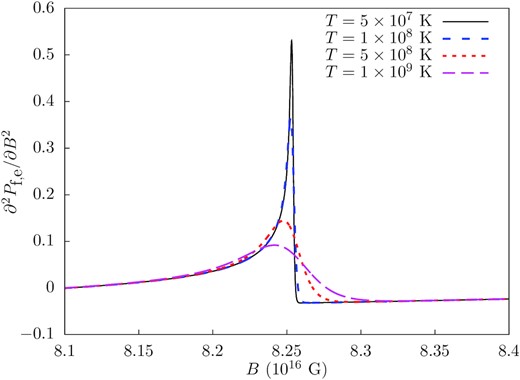
∂2Pf, e/∂B2 in units of c2 near where a new Landau level begins being filled for μe = 125 MeV, computed using the finite temperature-including form of Pf, a, equation (42). The explicit expression for ∂2Pf, e/∂B2 at finite T is given by equation (B3c). The damping effect of increasing temperature is clearly demonstrated.
For gσ/mσ, gω/mω, gρ/mρ, bσ, cσ, we use the tabulated parameters for the nuclear compressibility K = 300 MeV, m*/mN = 0.78 at saturation density σωρ model from table 5.5 of Glendenning (1997); these are gσ/mσ = 3.024 fm, gω/mω = 2.195 fm, gρ/mρ = 2.189 fm, bσ = 3.478 × 10⁻³, cσ = 1.328 × 10⁻². Unlike the reference, we do not include hyperons as our stellar model does not reach the densities at which they appear. The maximum Tolman–Oppenheimer–Volkoff (TOV) mass possible with this EOS is only ≈1.7 M⊙, so it does not cover the entire range of observed neutron star masses, but it does allow us to discuss MHD stability inside a reasonable model of a neutron star core.
4.1 Changes of variable and connection to magnetohydrodynamics
Because it is derived in the framework of quantum statistical mechanics using the grand canonical ensemble, the expression for P is in terms of chemical potentials of the fermions as opposed to their number densities. This is inconvenient for hydrodynamics where we work with conserved currents and fixed (number) densities and not at fixed chemical potentials. To compute the thermodynamic partial derivatives uB, uBB, uρB, uBY, and uBf which appear in the stability criteria and which are computed at fixed ρ, Y, f and/or B, we must first relate the pressure P, or more generally ΩG of equation (44), to the internal energy density defined in equation (1).
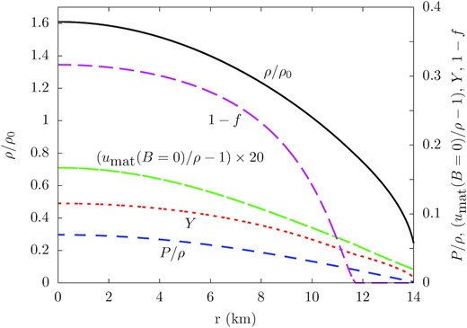
Properties of the neutron star model used to analyse the MHD stability: the mass density ρ divided by nuclear saturation density ρ0 = 2.7 × 10¹⁴ g cm−3, pressure P divided by ρ, the fractional difference between the internal energy density of the matter umat at B = 0 and ρ (scaled by a factor of 20), the proton fraction Y and one minus the electron fraction f. Only the properties within 14 km (ρ > 0.25ρ0) are shown, as the crust-core transition is expected to occur before these densities and a different EOS would be needed in this region.
4.2 Background stellar model
The evaluation of the stability criteria in Section 3 requires a background equilibrium fluid configuration which is perturbed according to the Lagrangian displacement field ξi. For this background model, we use a canonical neutron star with mass M* = 1.4 M⊙ and structure determined by the σωρ EOS discussed earlier. The presence of the magnetic field changes the stellar equilibrium, since the equation of hydrostatic balance for the background star is equation (3) with vi = 0. If the magnetic forces are small compared to the mechanical pressure, which is true for P ≫ BH/(8π), the magnetic forces will have a negligible effect on the stellar structure. For even the strongest fields B = 1017 G that we employ in this paper, this will be approximately true, with (1017G)2/(8π) at most a few per cent of the central pressure of the stellar model. Hence, when computing the background stellar model we use to find the gravitational acceleration g and the species gradients that appear in the Brunt–Väisälä frequency, we ignore the effect of the magnetic field.
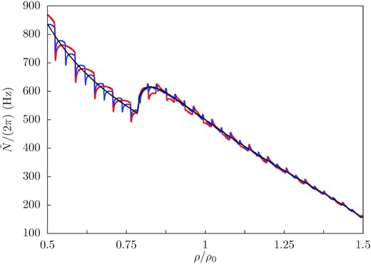
Brunt–Väisälä frequency with magnetic contributions |$\tilde{N}$| as a function of density for three different magnetic field strengths: B = 1015 G (black), B = 5 × 10¹⁶ G (blue), B = 1017 G (red). ρ0 = 2.7 × 10¹⁴ g cm−3. The bump starting at ρ = 0.79ρ0 is the leptonic buoyancy contribution that occurs where muons are present in the star.
We convert this field to Cartesian coordinates in line with our local analysis: the ϕ-direction is changed to the x-direction and the (spherical) radial direction is changed to the z-direction. Equation (78) hence implies d/dzln (B/ρ) = 1/z and d/dzln B = dln ρ/dz + 1/z. Since we are free to choose B0, we will pick values of B independent of the radial position and density with the understanding that B0 can be chosen appropriately to satisfy equation (78). Based on the density profile in Fig. 2, the maximum value of B within the core is ≈0.42B0.
5 NUMERICAL CALCULATION OF STABILITY CRITERIA
The properties of the stellar model discussed in Section 4.2 and the thermodynamic derivatives of uM discussed in Section 4 are the only inputs required to compute the local stability criteria from Section 3. Before doing so, we compute the first and second-order partial derivatives of uM with respect to B and ρ. In Fig. 4, we plot H, |$c_s^2$|, BρuρB, and B2uBB/ρ as a function of B or ρ, for a representative core temperature for a magnetar over a few hundred years old (Potekhin & Chabrier 2018) of 108 K. Panel (a) shows that B ≈ H as mentioned in the introduction, and prominently shows the de Haas–van Alphen oscillations of H, resulting from the population of successive Landau levels as B is decreased, where a new Landau level starts being populated significantly at |$B=(\mu _a^2-m_a^2)/(2en)$| for integer n. At T = 0, the slope of H(B) is discontinuous at |$B=(\mu _a^2-m_a^2)/(2en)$| for integer n; non-zero T restores continuity. However, the derivatives of H(B) fluctuate rapidly with large positive and negative values near |$B=(\mu _a^2-m_a^2)/(2en)$|. As the inset in (b) shows, the Landau quantization of the fermions also has a small effect on the sound speed, causing fluctuations of a few per cent around its zero field value. Landau quantization also results in the spikes that are observed in BuρB and B2uBB/ρ for B ≳ 1015. BuρB and B2uBB/ρ can clearly be negative, which will lead to potential instabilities. Since their sign change is associated with Landau quantization, we conclude that this will be the dominant mechanism in any potential instability that will occur as opposed to the vacuum Euler–Heisenberg Lagrangian. However, BuρB and B2uBB/ρ are much smaller than |$c_s^2$|, so it is clear that V2 defined in equation (19) will be positive, and so for the kx = 0 perturbations to be unstable will require the kx = 0 magnetic buoyancy criterion SC1 (equation 23) to be negative.
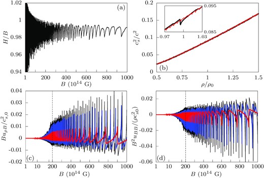
(a) H/B as a function of B- this is comparable to Broderick et al. (2000), Fig. 2. The fine details visible at B ≳ 7 × 10¹⁶ G are due to including multiple fermion species; the overall curve is dominated by the Landau quantization of the electrons. (b) |$c_s^2/c^2$| as a function of mass density for B = 1016 G (red) and B = 1017 G (black). The inset shows the small fluctuations in |$c_s^2$| due to Landau quantization. (c) |$Bu_{\rho B}/c_{s,0}^2$| as a function of B, where |$c_{s,0}^2\equiv 0.09c^2$| is the approximate sound speed squared at nuclear saturation density ρ0. The three curves are computed for fixed μe = 80 MeV (red), 125 MeV (blue) and 150 MeV (black), corresponding to ρ ≈ 0.56ρ0, ρ0 and 1.34ρ0, respectively. (d) |$B^2u_{BB}/(\rho c_{s,0}^2)$| as a function of B. The three curves are computed for the same values of μe as panel (d). Note the change from logarithmic to linear scaling of the horizontal axis at B = 2 × 10¹⁶ G, separated by a dotted line, in (c) and (d). All curves shown were computed using T = 108 K.
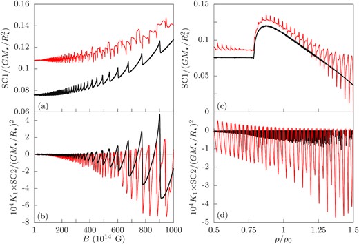
The quantity K1 defined in equation (27) and rewritten in equation (33) is plotted in Fig. 5 for a range of reasonable neutron star core temperatures T = 5 × 10⁷, 108, 5 × 10⁸ K. The damping effect of increasing temperature is clearly demonstrated, but is important only where new Landau levels become populated i.e. where the second-order partial derivatives of P would be divergent at zero temperature. Increasing the temperature stabilizes the fluid; as the temperature is increased, fewer ‘spikes’ in K1 become negative. The unstable regions are very narrow in B-space for constant ρ and in ρ-space for constant B.

The MPR stability criterion K1 defined in equation (19) divided by |$c_{s,0}^2$| as a function of B (a,b) and ρ (c,d) for T = 5 × 10⁷ (black), 108 K (blue), and 5 × 10⁸ K (red). Values below the thin grey line (i.e. negative values) are unstable. μe = 80 MeV (ρ ≈ 0.56ρ0) and μe = 125 MeV (ρ ≈ ρ0) are used in (a) and (b), respectively; note the change from logarithmic to linear scaling of the horizontal axis at B = 2 × 10¹⁶ G, separated by a dotted line. B = 5 × 10¹⁶ and 1017 G are used in (c) and (d). The Alfvén velocity squared BH/(4πρ) ≈ B2/(4πρ), also divided by |$c_{s,0}^2$|, is shown as a dot–dashed line in each panel. The irregular-looking behaviour that occurs in (c) and (d) for ρ > 0.79ρ0 is due to the presence of the muons, which misaligns the Fermi momenta of the protons and electrons. Additional evidence of this effect can be seen by comparing (a) and (b), since (a) is at a density below the muon threshold and (b) is above it.
Because |$c_s^2$| can be so large, the behaviour of K1 is dominated by the first term in equation (33). This term is approximately the Alfvén velocity squared, multiplied by a factor which can change sign because uBB can be negative (Fig. 4d). The fluctuations of uBB are responsible for K1 < 0 in parts of B–ρ parameters space, indicating a possible MPR instability. Increasing B at fixed density makes K1 more stable, while increasing density at fixed B leads to further unstable regions in parameter space. Recall that Alfvén waves have magnetic tension as their restoring force, and that likewise there is a magnetic pressure contribution to the restoring force for standard magnetosonic waves. Intuitively, the instability occurs because the (1 + 4πuBB) factor multiplying |$B^2/\rho \propto v_{\text{A}}^2$| becoming negative corresponds to an effective negative magnetic tension/pressure. Thus, changes in the field strength or direction in these unstable regions are energetically favourable, if the (always positive) sound speed (i.e. the matter pressure) is unable to stabilize the fluid. We discuss ways around stabilization by the sound speed at the conclusion of this section.
In Fig. 6, K1 is plotted in the neutron star core for the field in equation (78) with specific values of B0. The maximum field inside the star is ≈0.42B0. For fixed B, the higher density regions are more unstable (have more negative K1), and as B is increased, higher densities are required for the fluid to become unstable at all (cf. Fig. 5c and d). For fixed ρ, instability can occur at intermediate fields – as B → 0, the fluid is stable, and for sufficiently high fields it can also become stable (cf. Fig. 5a and b), with the field required to stabilize the fluid increasing with increasing density.
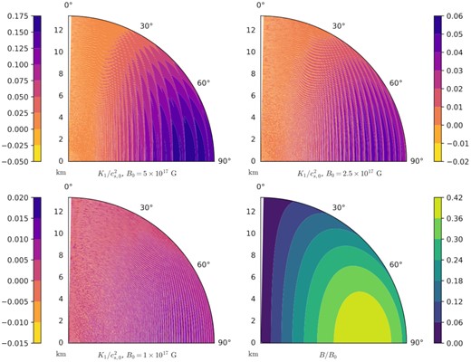
|$K_1/c_{s,0}^2$| for different values of B0, and B/B0 (lower right), for a cross-section of the model stellar core at T = 5 × 10⁷ K. Negative values correspond to unstable regions. Instability is associated with negative values that occur near lines of |$(\mu _{\text{e}}^2-m_{\text{e}}^2)/(2eB)=$| an integer. Note that some of the small-scale structure at high densities is spurious and due to interpolation based on a limited sampling in B–ρ parameter space, and that the region along the symmetry axis θ < 1° was excluded as B vanishes here.
The unstable regions are localized in spheroidal shells where |$B=(\mu _a^2-m_a^2)/(2en)$| for a fixed integer n is satisfied – as n increases (e.g. with increasing density) these shells become more closely spaced, leading to the appearance of nearly continuously unstable regions deep in the core. This is observed in Fig. 6 as the field is decreased from the B0 = 5 × 10¹⁷ G to the B0 = 2.5 × 10¹⁷ G to the B0 = 1 × 10¹⁷ G subfigures: the spacing between the unstable regions decreases, to the point that it is difficult to distinguish these regions in the B0 = 1 × 10¹⁷ G subfigure. However, these locations are not required to be unstable, since for sufficiently strong B/sufficiently high temperature, they will be stable (cf. Fig. 5a and b). This leads to the highest field regions in the B0 = 5 × 10¹⁷ subfigure of Fig. 6 being stable. Fig. 7 shows a magnified section of the B0 = 5 × 10¹⁷ G, T = 5 × 10⁷ K stellar model; the alternating pattern of stable and narrow unstable regions is more apparent here.
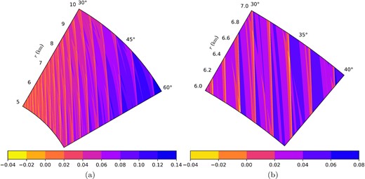
(a) |$K_1/c_{s,0}^2$| for a slice of a stellar core model seen in Fig. (6) (B0 = 5 × 10¹⁷ G, T = 5 × 10⁷ K); a further magnified section is shown in (b). This shows the fine details of the narrow unstable regions.
Now that the behaviour V2 and K1 is understood, we examine the other stability criteria. In Fig. 8, we show the kx = 0 stability criterion equation (23) (SC1) and the first kx ≠ 0 criterion equation (32a) (SC2). In Fig. 8, we show the two kx ≠ 0 criteria equations (32b)–(32c) (SC3,SC4). We note again that SC1, SC3, and SC4 are associated with magnetic buoyancy, while SC2 is a purely MHD stability criterion. SC2, SC3, and SC4 have all been multiplied by a factor K1 to eliminate the divergent behaviour for K1 → 0: since K1 < 0 is already potentially unstable, such regions have been excised from the plots of SC2, SC3, and SC4.
The magnetic buoyancy stability criterion for kx = 0 defined in equation (23) (SC1), and the stability criterion SC2 defined in (32a), as functions of B (a,b) and ρ (c,d). Each quantity is scaled by appropriate factors of G, M⋆, and R⋆ to make them dimensionless, while SC2 is multiplied by K1 to eliminate divergent behaviour and an additional factor of 104. In (a) and (b), the black and red curves correspond to μe = 80 MeV (ρ ≈ 0.56ρ0) and μe = 125 MeV (ρ ≈ ρ0), respectively. In (c) and (d), the black and red curves correspond to B = 1015 and 5 × 10¹⁶ G, respectively. All curves are computed at T = 5 × 10⁸ K. The B = 1015 G curve in (d) is multiplied by an additional factor of 2000 (on top of the other factors) for display purposes.
SC1 is always positive in the stellar model we have considered, and hence the fluid and field configuration we examine is magnetic buoyancy-stable for kx = 0 perturbations (i.e. purely radial perturbations). The stable stratification is large enough to suppress the instability i.e. |$\tilde{N}$| is large enough to overwhelm the second term in equation (23), which is proportional to the same term which results in negative values of K1 and which could destabilize the system for sufficiently small |$\tilde{N}$|. This demonstrates the importance of stable stratification to MHD stability even in the strong-field case. SC2, SC3, and SC4 all involve K1, which we have seen undergoes large fluctuations and can change sign for fields ≳1015 G. Also note the similarities between Fig. 3 and Figs 8 and 9 panel (c), as the latter depend on scaled versions of |$\tilde{N}^2$|.

The magnetic buoyancy stability criteria defined in equation (32b) (SC3) and (32c) (SC4), as functions of B (a,b) and ρ (c,d). Each quantity is scaled by appropriate factors of G, M⋆, and R⋆ to make them dimensionless, and both are multiplied by K1 to eliminate divergent behaviour. SC4 is scaled by an additional factor of 104. In (a) and (b), the black and red curves correspond to μe = 80 MeV (ρ ≈ 0.56ρ0) and μe = 125 MeV (ρ ≈ ρ0), respectively. In (c) and (d), the black, red, and blue curves correspond to B = 1015, 5 × 10¹⁶ and 1017 G, respectively. All curves are computed at T = 5 × 10⁸ K. The B = 1015 G curves in (c) and (d) are multiplied by an additional factor of 100 and 10 000, respectively (on top of the other factors) for display purposes.
SC2, SC3, and SC4 can all be negative in large parts of the B–ρ parameter space, contrasting with the limited regions of the parameter space in which K1 can be negative which are localized at where additional Landau levels start filling. The region of parameter space where SC2 is negative increases as B and ρ are increased, as is demonstrated in Fig. 10, where K1 ×SC2 is plotted in a cross-section of the stellar model. SC3 is negative in limited regions where additional Landau levels start being populated, and also for regions where B ≳ 6 × 10¹⁶ G and ρ ≲ 0.8ρ0. The latter SC3 < 0 regions are due to the second term in equation (34), since the |$\text{d}\ln B/\text{d}z=\text{d}\ln \rho /\text{d}z+\frac{1}{z}$| is the most negative at low densities (see Fig. 2) and the coefficient of this derivative becomes large for large B. SC4 is generally positive or marginally negative at B ≲ 2 × 10¹⁶ G, and can be unstable for all densities examined.
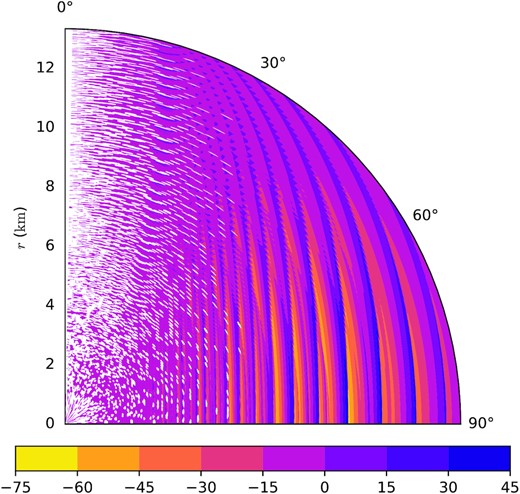
104K1 ×SC2/(GM⋆/R⋆)2 for the stellar core model with B0 = 5 × 10¹⁷ G and T = 5 × 10⁸ K. Negative values correspond to potentially unstable regions. The empty regions correspond to where K1 < 0 and the fluid is already unstable to the MPR instability – such regions correspond to the unstable regions in the upper left plot of Fig. 6, though not every K1 < 0 region is resolved in each figure.
In the case where the buoyancy terms SC3 and SC4 are relevant, these can further destabilize the fluid, but like K1 and SC2 will require a particular class of perturbation (e.g. incompressible) to overcome the stabilizing effect of the sound speed squared term in equation (85). However, the pure MHD terms are much more significant for the stability than those associated with buoyancy except for the longest wavelength perturbations. The minimum relevant wavenumber for a perturbation is kmin ≈ 2π/R⋆ ∼ 4 × 10⁻⁶ cm−1, at which point |$K_1k_{\text{min}}^2\sim$|SC2|$k_{\text{min}}^2\sim$|SC3. For shorter wavelength perturbations, the wavenumber dependence of the pure MHD terms mean that they will be much larger in magnitude than the magnetic buoyancy terms.
6 DISCUSSION AND CONCLUSION
In this paper, we have extended the MHD stability analysis of Friedman & Schutz (1978) and Glampedakis & Andersson (2007) to magnetizable fluids with B ≠ H, and applied this to the study of MHD stability in the presence of extremely strong fields where QED effects and Landau quantization of fermions are relevant. This regime is important to magnetars, which have surface fields ∼1015 G and likely stronger fields in their interiors. Using the canonical energy approach to studying stability, we determined sufficient local stability criteria for magnetic buoyancy, magnetosonic stability, and the MPR instability for magnetizable media with an electromagnetic Lagrangian depending on the magnetic field B, mass density ρ and species fractions Ya. The fluid perturbation theory and canonical energy results derived here are general and can be used for other applications where H ≠ B e.g. superfluid-superconducting neutron stars.
We find that the inclusion of strong-field effects to the MHD of a neutron star core leads to a possible MPR instability associated with the Landau quantization of fermions for fields B ≳ 1015 G and at typical core densities. These instabilities can have growth times of the order of 10−3 s, and are not stabilized by viscous dissipation under expected neutron star viscosities. The magnetic buoyancy instability associated with the strong-field, B ≠ H MHD studied here can also be active in the neutron star core, and the stability criteria associated with it are violated in broader regions of the B–ρ parameter space than the narrow regions in which the MPR instability criterion is violated. However, these terms are only comparable in magnitude to the purely MHD terms associated with the MPR instability for long wavelength perturbations, and are unimportant for stability at shorter wavelengths. The vacuum Euler–Heisenberg Lagrangian was found to be unimportant to MHD stability overall at the magnetic fields B ≲ 1017 G we considered.
Perhaps the most important question regarding the MPR instability discussed in this paper is what implications it has on the evolution of magnetar fields. The alternating stable-unstable regions in B–ρ space, demonstrated in a stellar model in Figs 6 and 7, suggest that the instability could lead to the formation of magnetic domains. This instability will likely be triggered throughout the star’s life for two reasons: (1) previously stable regions become unstable as the star cools and the ‘spikes’ in uBB become sharper (cf. Fig. 5); (2) field evolution that changes the field strength within the star such that certain regions now lie in the unstable parts of B–ρ parameter space. One response to this destabilization is the transfer of magnetic flux from unstable regions until the local field is in the stable region of the B–ρ parameter space. Since the unstable regions themselves generally span very narrow length scales of the order of ≲metres, the magnetic field only needs to change by a small fraction of its strength to be stabilized, so unstable modes could transfer flux to stabilize the fluid. This suggests that the observational implications for these domains and the instability that could form them are limited, at least within the stellar core.
The formation of magnetic domains in strongly magnetized neutron star matter has previously been discussed in Blandford & Hernquist (1982) and Suh & Mathews (2010). In these calculations, it is the differential magnetic susceptibility χ, corresponding here to −uBB,2 which encourages magnetic domain formation, and when χ > 4π the system is thermodynamically unstable to domain formation. The MPR instability discussed in our paper also originates from uBB < −1/(4π), in contrast to the original MPR instability in superconducting fluids that depends on the |$u_{\rho B}^2$| term in K1. Magnetic domain formation encouraged by the instability discussed here suggests that smoothly varying fields are not solutions to the background magnetohydrostatic equilibrium for sufficiently strong magnetic fields ≳1015 G and at low temperatures.
Though we have made some simplifying assumptions for the background stellar model, our conclusions about the MPR instability arising from the Euler–Heisenberg–Fermi–Dirac Lagrangian should be robust. This is because the instability depends on uBB, which is simply a function of B and the na (or the μa), and is independent of the exact structure of the star (including the EOS) or the magnetic field direction. We thus do not expect our main argument about the generic instability of ultrastrong fields to change significantly when using a relativistic stellar model, different EOS and/or including the effect of the magnetic field on the background equilibrium model. Our restriction to toroidal fields does not affect our main results about the instability to MPR modes, since the same requirements on K1 will appear independent of the direction of Bi: if Bi was a poloidal field, only the magnetic buoyancy conditions, and the exact location of the unstable regions within the star, would be changed.
The next logical step is to apply this formalism to the crust (Rau & Wasserman, in preparation), which due to lower densities and sound speeds may support similar instabilities as in the core even with lower field strengths. However, the stability analysis in the crust is fundamentally different due to the lack of a canonical energy procedure (Lyutikov 2013), so this is left to a follow-up paper. The canonical energy procedure can also be applied to a complete model of a neutron star core to study its global stability. An additional interesting area of future study would be to include a physically correct stellar exterior, which would modify the treatment of the surface terms examined in Appendix A2, in which exterior vacuum was assumed. Such a study could examine the effect on the stability of different pulsar magnetosphere models and could potentially help judge their feasibility.
SUPPORTING INFORMATION
APPENDIX A. Fluid Perturbation Theory.
APPENDIX B. Thermodynamic Derivatives Of Euler–Heisenberg–Fermi–Dirac Lagrangian.
Please note: Oxford University Press is not responsible for the content or functionality of any supporting materials supplied by the authors. Any queries (other than missing material) should be directed to the corresponding author for the article.
ACKNOWLEDGEMENTS
We would like to thank the referee for useful comments. PBR would also like to acknowledge the support of Cornell’s Boochever Fellowship for spring 2020.
DATA AVAILABILITY
The data underlying this article will be shared on reasonable request to the corresponding author.
Footnotes
The zeroth space–time component of the ω meson and the zeroth space–time component of the I3 isospin component of the ρ meson – the ‘3’ superscript on |$\rho ^3_0$| denotes the isospin component and not exponentiation.
Though noting the other references perform the calculation of the differential susceptibility at fixed chemical potentials and not fixed density as used here.
