


ABSTRACT
We use a large K-selected sample of 299 961 galaxies from the REFINE survey, consisting of a combination of data from three of the deepest near-infrared surveys, UKIDSS UDS, COSMOS/UltraVISTA, and CFHTLS-D1/VIDEO, that were homogeneously reduced to obtain photometric redshifts and stellar masses. We detect 2588 candidate galaxy groups up to z = 3.15 at S/N > 1.5. We build a very pure (|$\gt 90{{\rm \,per\ cent}}$|) sample of 448 candidate groups up to z = 2.5 and study some of their properties. Cluster detection is done using the DElaunay TEssellation ClusTer IdentiFication with photo-z (detectifz) algorithm that we describe. This new group finder algorithm uses the joint probability distribution functions of redshift and stellar-mass of galaxies to detect groups as stellar-mass overdensities in overlapping redshift slices, where density is traced using Monte Carlo realization of the Delaunay Tessellation Field Estimator. We compute the algorithm selection function using mock galaxy catalogues taken from cosmological N-body simulation lightcones. Based on these simulations, we reach a completeness of |$\sim \! 80{{\,\rm per\ cent}}$| for clusters (M200 > 1014M⊙) at a purity of |$\sim \! 90{{\, \rm per\ cent}}$| at z < 2.5. Using our 403 most massive candidate groups, we constrain the redshift evolution of the group galaxy quenched fraction at 0.12 ≤ z < 2.32, for galaxies with 10.25 < log M⋆/M⊙ < 11 in 0.5 × R200. We find that the quenched fraction in group cores is higher than in the field in the full redshift range considered, the difference growing with decreasing redshift. This indicates either more efficient quenching mechanisms in group cores at lower redshift or pre-processing by cosmic filaments.
1 INTRODUCTION
The formation and evolution of galaxies, and the clusters and groups where a large fraction of them inhabit and are intimately related, have implications for many different areas of astrophysics and cosmology. Ever since the earliest studies by Messier (1781), it has increasingly becoming established that galaxies cluster and group together and are not just randomly distributed on the sky. Soon after this there were hints of an evolutionary connection between galaxies and their environments. The major work which set off the modern study of this relation was Dressler (1980), who showed that galaxies are more likely to be passive, older, and early type in dense local environments than in lower density ones. This later has been expanded to include other features of galaxies such as star formation (Gómez et al. 2003), such that it is clear that galaxies in dense environments have a different star formation rate (SFR) than similar mass galaxies in lower density environments.
Therefore for decades it has been clear that galaxies are more evolved in denser areas than in lower density environments, at least at redshifts z < 1. This implies that star formation is quenched earlier, or somehow does not continue, in galaxies found in high-density environments compared with those in low-density environments. In general, either galaxies finish their star formation earlier and no gas is replenished in dense environments due to gas exhaustion/strangulation (Larson, Tinsley & Caldwell 1980), or the environment itself is driving the reduction or removal of star formation such as through process including ram-pressure stripping (Gunn & Gott 1972) and high-speed galaxy encounters (Moore et al. 1996). Many recent studies find this relation appears to hold even at 1 < z < 1.5, some of the highest redshifts in which large enough samples of clusters can be found (see e.g. Quadri et al. 2012; Cooke et al. 2016; Nantais et al. 2016; Papovich et al. 2018; van der Burg et al. 2020). However, there is considerable debate about the existence of a turn-over in this relationship at higher redshifts where clusters are not so easily found (e.g. Elbaz et al. 2007; Lani et al. 2013; Nantais et al. 2016), and thus the picture is not as clear for lower density environment such as groups.
Major questions relating to the formation of the earliest clusters pertain not only to the formation and quenching of galaxies, but also to the existence and formation of clusters themselves which can have cosmological implications (see Allen, Evrard & Mantz 2011 for a review). In general, we find that galaxy evolution occurs via both internal and external mechanisms and forces. The environments in which a galaxy finds itself must have a strong effect on how it forms and evolves, simply due to the range of environments galaxies are located within and the physical effects of those environments. An example of this is galaxies surrounded by other galaxies in close proximity such as those involved in galaxy mergers (e.g. Duncan et al. 2019). In these cases, gravitational interactions and mergers induce star formation and dynamical processes that can, in the right conditions, remove stars/gas through tides. As such, the masses of galaxies can increase through accretion of satellites and the number of galaxies decreases due to mergers. Furthermore, there can be changes to the structures and morphologies of galaxies due to this close proximity and high-speed encounters (e.g. Mastropietro et al. 2005). Dense areas such as clusters also often contain an intracluster medium – gas in the space between the galaxies in a group. This intracluster gas can interact with the gas located within galaxies themselves through ram-pressure stripping. This mechanism strips the galaxy of its cold gas, thus preventing further star formation. This process that has been extensively observed in galaxy clusters (e.g. Scott et al. 2012; Gavazzi et al. 2018; Vulcani et al. 2020) can be very efficient in this environment, shutting down star formation on time-scales of tens of Myr (Abadi, Moore & Bower 1999), and it may be the dominant galaxy evolution mechanism in massive clusters (see Boselli & Gavazzi 2014 for a review). Even though this mechanism has been recently observed in galaxy groups in the local universe (Vulcani et al. 2018), its efficiency in groups is thought to be limited (e.g. Rasmussen, Ponman & Mulchaey 2006). However, the lower density intragroup gas can still efficiently strip the gaseous halo surrounding galaxies that is not as strongly gravitationally bound to it. When this happens, and because gas cannot be replenished after all the existing gas is used up in star formation, a galaxy will become ‘passive’ and lose its structure due to faded star formation (e.g. Wetzel et al. 2013; Peng, Maiolino & Cochrane 2015). Even lower density cosmic web filaments have been shown to be favourable environments for suppressing star formation (e.g. Kuutma, Tamm & Tempel 2017; Kraljic et al. 2018; Laigle et al. 2018) with different quenching mechanisms proposed (Aragon Calvo, Neyrinck & Silk 2019; Song et al. 2021).
Previous results show that for the most part the properties of galaxies are determined by both their environment and the individual mass of a galaxy (e.g. Peng et al. 2010, at z < 1). Therefore, there are two ways to prevent further star formation from taking place within a galaxy – either a dense environment, which due to a rich intracluster environment quenches the star formation or quenching due to containing a high mass – so-called mass quenching (e.g. Peng et al. 2010; Bluck et al. 2019). For the lowest mass galaxies, it is likely that the rich environment is mostly responsible for quenching, but for higher mass galaxies, the situation is more complicated (e.g. Grützbauch et al. 2011a). Moreover, while the efficiency of massive galaxy clusters in quenching star formation at z > 1 has become clearer in recent years (Nantais et al. 2016; van der Burg et al. 2020), the ability of high redshift groups to do so is still unclear. Similarly, examining the morphology–density relationship at z < 1, Tasca et al. (2009) showed that the morphology–density relation evolves slightly with redshift, becoming flatter and less strong at higher-z (see also Grützbauch et al. 2011a,b), and is most likely responsible for producing low-mass galaxy morphology, while stellar mass seems to play a more important role for massive galaxy morphology. The morphology results are also backed up by finding a kinematic-structure/environment relation (Brough et al. 2017). The question however remains, which relationship – mass or environment – is more fundamental (e.g. Grützbauch et al. 2011a)? This relates to, and is another way of addressing, the nature versus nurture problem for galaxy formation.
We can address this question by examining the stellar populations, structures, and morphologies of galaxies within higher redshift overdensities, or within proto-clusters that are just forming (e.g. Dressler et al. 1997; Holden et al. 2007; Sazonova et al. 2020). However, observations of overdensities at high redshifts z > 1.5 are just starting in earnest, but already the observations available gives us some ideas of how this evolves. What we know so far is that massive clusters at high redshifts, up to z ∼ 1.2, display a similar morphology–density relation as local galaxies, such that denser areas of galaxies contain higher fractions of elliptical systems. However, what is also seen is that the normalization is lower, such that at a given density there are fewer ellipticals than at the same local density at lower redshifts (e.g. Sazonova et al. 2020). It is also known that the quenched fraction is higher in massive clusters up to z = 1.5 (e.g. Lin et al. 2017; Sarron et al. 2018; van der Burg et al. 2018, 2020). This is seen as a stronger effect for low-mass galaxies, but steadily decreases with increasing redshift. At higher redshifts 1.5 < z < 2, few massive clusters have been studied but these can exhibit quenched fractions as high as |$\sim \! 75{{\ \rm per\ cent}}$| (Newman et al. 2014; Strazzullo et al. 2019).
What is now needed is a systematic search for distant clusters and groups, both as a way to find clusters and to study their galaxy populations, but also to determine the best ways to maximize the purity and completeness of samples of groups/clusters. There have been few such studies (e.g. Papovich 2008; Audrey et al. 2012; Chiang, Overzier & Gebhardt 2014; Rettura et al. 2014; Ando, Shimasaku & Momose 2020) and many of them are biased by severe selection effects due to detection process targeting specific galaxy properties (e.g. colour selection or radio activity, see Overzier 2016, for a review on high redshift overdensity and (proto-)cluster detection). Among the many ways to search for distant galaxy clusters, perhaps the cleanest way is to search for overdensities of galaxies in a limited area. In this sense, we are simply looking for multiple galaxies that have similar redshifts and are found in the same part of the sky.
Thus, in this paper, we carry out a new analysis of the three deepest extragalactic deep fields measured to date – the UltraVISTA, the UKIDSS Ultra-Deep Survey (UDS) and the VIDEO surveys to find the most distant and massive clusters within the deepest ground-based imaging fields. In many ways, this analysis is a precursor to what can be done with large forthcoming imaging surveys, such as Euclid, Rubin and Roman. Our goals in this paper are to provide a catalogue of sources, analyse the likelihood of galaxies being members of clusters through simulations, and provide a frame-work for investigating the ability to find z > 1.5 groups and clusters and study galaxy properties therein in future deep surveys such as Euclid and Rubin which will have similar depths, but cover thousands of times more area.
This paper is organized as follows. In Section 2, we explain the data that we use in this paper, including the mock data. In Section 3, we explain our new algorithm – the detectifz method for finding overdensities. Section 4 includes our group and cluster finding results, including a discussion of the catalogue of sources which we find. Section 5 presents the evolution of the quenched fraction for galaxies as a function of redshift which are discussed in Section 6. We use AB magnitudes throughout the paper and assume a flat ΛCDM cosmology with Ωm = 0.3 and h = 0.7.
2 DATA AND MOCK DATA
The data products for this study are those which arise from the REFINE (Redshift Evolution and Formation in Extragalactic systems) project, which is essentially a re-derivation and homogenization of the major ground-based data sets used to study the distant Universe (see e.g. Mundy et al. 2017). As such, this paper is based on the data products presented in Mundy et al. (2017) for the UKIDSS Ultra Deep Survey (UDS), COSMOS/UltraVISTA, and CHFTLS-D1/VIDEO survey regions. Mundy et al. (2017) computed photometric redshift probability distribution functions (PDFs) using the eazy photometric redshift code (Brammer, van Dokkum & Coppi 2008) and stellar masses using an old version of the SED-fitting code smpy (presented in Duncan et al. 2014). Throughout this work, we use the eazy photometric redshifts (zphot and PDF(z)) computed by Mundy et al. (2017). We refer to Mundy et al. (2017) for details on how the photometric redshifts were obtained and detailed comparison to spectroscopic redshift samples. In contrast, we do not use Mundy et al. (2017) stellar-mass estimates but instead our own rederivation of galaxy stellar-masses based on a newer version of smpy (Duncan et al. 2019). We detail in Section 2.2 how these new stellar-mass estimates are obtained and briefly summarize the main characteristics of the data and of these data products in the three survey regions in Sections 2.1.1–2.1.3. Below we give more detail about our derived data products and what we have done to create these and optimize them for our own purposes.
2.1 Data sources
Our data sources arise from three different fields – the UKIDSS Ultra Deep Survey (UDS), the UltraVISTA survey of the COSMOS field, and the deep VIDEO field. These data sources are part of the REFINE survey for exploring galaxy evolution on deep ground-based data.
2.1.1 UKIDSS Ultra Deep Survey (UDS)
We use the data aggregated by Mundy et al. (2017) in the UKIDSS Ultra Deep Survey (UDS). It is based on the eighth data release of UDS, the deepest field of the UKIRT Infra-Red Deep Sky Survey (UKIDSS; Lawrence et al. 2007) that covers 0.77 deg2 and obtained deep photometry in J, H, K to limiting AB magnitudes of 24.9, 24.2, and 24.6, respectively, in 2 arcsec apertures. Complementary observations were aggregated from the CFHT MegaCam u, BVRiz from Subaru XMM Deep Survey, Y from ESO VISTA Survey Telescope, IR photometry in four channels from the Spitzer Legacy Program for a combined wavelength range 0.3 < λ < 4.6 |$\mu$|m.
The catalogue we use was selected by Mundy et al. (2017) in the K band at |$99{{\ \rm per\ cent}}$| completeness K = 24.3. It contains ∼90 000 galaxies out to z ∼ 3.5 (|$90{{\ \rm per\ cent}}$| of galaxies are at z < 2.4) in an effective area of 0.63 deg2.
Mundy et al. (2017) photometric redshifts have a σNMAD = 0.053 × (1 + z) and outlier rate of |$\eta = 5{{\ \rm per\ cent}}$| compared to a sample of spectroscopic redshifts. Median 1σ uncertainties on their rescaled PDF(z) is σPDF(z) = 0.040 × (1 + z), considering all galaxies |$90{{\ \rm per\ cent}}$| complete in stellar mass.
2.1.2 COSMOS/UltraVISTA
We also use the photometric data aggregated by Mundy et al. (2017) in the COSMOS/UltraVISTA survey. It is based on the publicly available Ks-selected catalogue of Muzzin et al. (2013) that observes the COSMOS field (Cosmological Evolution Survey; Scoville et al. 2007) with the ESO Visible and Infrared Survey Telescope for Astronomy (VISTA) telescope and covers an effective area of 1.62 deg2. PSF-matched magnitudes obtained in 2.1 arcsec apertures are provided for 30 bands in the wavelength range 0.15 < λ < 24 |$\mu$|m. The catalogue was selected in the VISTA Ks band at |$90{{\ \rm per\ cent}}$| completeness magnitude of Ks = 23.4 and contains ∼150 000 galaxies out to z ∼ 3 (|$90{{\ \rm per\ cent}}$| of galaxies are at z < 1.8).
Mundy et al. (2017) photometric redshifts have a σNMAD = 0.013 × (1 + z) and outlier rate of |$\eta = 0.5{{\ \rm per\ cent}}$| compared to a sample of spectroscopic redshifts. Median 1σ uncertainties on their rescaled PDF(z) is σPDF(z) = 0.012 × (1 + z) considering all galaxies |$90{{\ \rm per\ cent}}$| complete in stellar mass.
2.1.3 CFHTLS-D1/VIDEO
We use data from the VISTA Deep Extragalactic Observations (VIDEO; Jarvis et al. 2012) in the near-IR Z, Y, J, H, Ks bands, matched to the 1 deg2 of the Canada–France–Hawaii Telescope Legacy Survey Deep-1 field (CFHTLS-D1) in optical u, g, r, i, z bands, covering the wavelength range 0.3 < λ < 2.1 |$\mu$|m. We use the VISTA Ks-selected catalogue of VIDEO June 2015 release cut at |$90{{\ \rm per\ cent}}$| completeness magnitude of Ks = 22.5 (see Mundy et al. 2017, for details on the completeness simulations) and contains ∼55 000 galaxies out to z ∼ 2.5 (|$90{{\ \rm per\ cent}}$| of galaxies are at z < 1.8).
Mundy et al. (2017) photometric redshifts of this field have a σNMAD = 0.044 × (1 + z) and outlier rate of |$\eta = 2.9{{\ \rm per\ cent}}$| compared to a sample of spectroscopic redshifts. Median 1σ uncertainties on their rescaled PDF(z) is σPDF(z) = 0.034 × (1 + z) considering all galaxies |$90{{\ \rm per\ cent}}$| complete in stellar mass.
2.2 Stellar masses
We obtain individual galaxy stellar mass estimates, using the SED-fitting code smpy in its version presented in Duncan et al. (2019). We use Bruzual & Charlot (2003) stellar population synthesis models with a Chabrier (2003) initial mass function (IMF). Galaxy model ages are allowed to vary between 10 Myr and 13.7 Gyr, sampled at 100 values equally spaced in logarithmic units, enforcing that the galaxy cannot be older than the age of the universe at the redshift under consideration in the fit. Metallicities of 0.005, 0.02, 0.2, 1, 1.75, and 2.5 Z/Z⊙ are considered. We assume Calzetti et al. (2000) dust attenuation curve with strength in the range 0 ≤ AV ≤ 4, linearly sampled at 12 values. We adopt exponential τ models for star formation histories (SFR∝e−t/τ) both decreasing (positive τ) and increasing (negative τ) with characteristic time-scales |τ| = 0.25, 0.5, 1, 2.5, 5, and 10 Gyr, with additional short burst τ = 0.05 and continuous (τ ≫ 1/H0) star-formation models, as in Duncan et al. (2019). As in Mundy et al. (2017), we do not include nebular emission. The redshift space is sampled at dz = 0.01 between z = 0.01 and z = 5, in line with photometric redshifts in Mundy et al. (2017). The simulated fluxes are compared to the total observed flux of our data galaxies using the method described in Duncan et al. (2019). The observed total flux in each filter is obtained from aperture flux as in Muzzin et al. (2013).
An example of such two-dimensional PDFs are shown in Fig. 1.
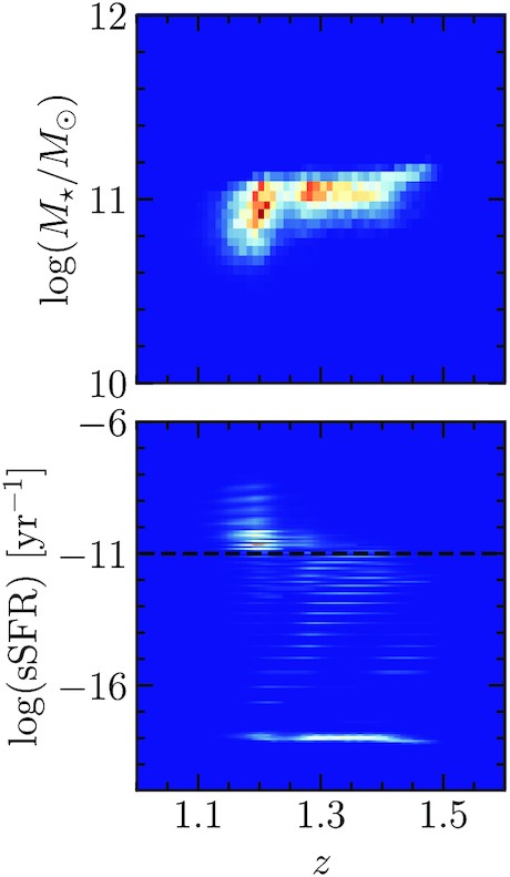
Examples of two-dimensional PDFs for one galaxy in VIDEO. Top: PDF(M⋆, z). Bottom: PDF(sSFR, z). The black dashed lines show the sSFR cut used to select quiescent galaxies in Section 5. Interestingly, this galaxy exhibits two regions of high probability in the parameter space that corresponds to similar z and M⋆ but very different sSFR.
In practice, as noted in López-Sanjuan et al. (2017) the probabilistic nature of the PDFs introduces correlations due to galaxies being spread over several bins. This renders binning necessary to account for these correlations and to obtain realistic number counts. López-Sanjuan et al. (2017) found that the optimal bin size is |$\Delta z = \frac{z_{\rm sup}-z_{\rm inf}}{2} = 2 \times \langle \sigma _z^{68}\rangle _{\rm median}(z)$|. They find the same scaling between bin size and the typical uncertainty for their absolute magnitude parameter, which is comparable in nature to our stellar-mass parameter. This bin size is also coherent with the choice of Castignani & Benoist (2016). In this work, we will use the |$95{{\ \rm per\ cent}}$| confidence interval (which is equal to 2σ is the normal approximation) as our bin size (see Section 5.1).
We will outline in the relevant sections how this information is used in each particular situation. This treatment of the information output by SED-fitting codes (eazy and smpy) allows us to statistically study galaxy properties without losing information. We stress that compared to the more classical approach that consists in using the best-fitting solution for redshift and stellar mass, and then using a strong cut on these point-estimates to select galaxies in a given range, our method allows us to properly treat uncertainties on galaxy physical parameter estimates (and their covariances).
2.2.1 Useful notations
Throughout the paper, we will use the notation |$\sigma ^{\rm CI}_X$|, which is the uncertainty on the point estimate of parameter X that corresponds to the CI confidence interval. For example, |$\sigma ^{68}_z$| is the uncertainty on photometric redshifts built from the |$68{{\ \rm per\ cent}}$| confidence interval as |$\sigma ^{68}_z = 0.5 \times (z_{u_{68}}-z_{l_{68}})$|, where |$z_{l_{68}}$| and |$z_{u_{68}}$| are, respectively, the lower and upper limit of the |$68{{\ \rm per\ cent}}$| confidence interval on PDF(z).
In several parts of this work (e.g. group detection, group galaxy membership probabilities and galaxy number counts), we need to estimate the typical uncertainty on a given parameter X at a given redshift z, stellar-mass M⋆ or at a given (M⋆, z). For example, we are interested in the typical redshift uncertainty |$\sigma ^{68}_z$| for galaxies of stellar mass M⋆ located at redshift z. While taking the median or the mean uncertainty is more common, we work with the |$68{{\ \rm per\ cent}}$| percentile of the individual uncertainty distribution, which we found to be better suited to maximize the efficiency of group detection. For clarity, throughout the paper this quantity is quoted using the following notation |$\langle \sigma ^{68}_z \rangle _{P_{68}}(M_\star ,z)$|.
We note |$\mathcal {N}(\mu , \sigma)$| the normal distribution of mean μ and standard deviation σ. Other distributions are explicitly named.
2.3 Mock data
To compute the selection function of our cluster finder algorithm and the reliability of our cluster membership assignments, we create semirealistic mock data sets resembling each survey region from cosmological simulation lightcones. We test these mocks in the same way we do our own data to see how well we can retrieve known galaxy clusters and groups at a variety of redshifts.
In recent years, some studies used simulated instrumental pipelines through which cosmological lightcones are observed to obtain mock observed photometric catalogues. Applying SED-fitting routines to these mock photometric catalogues, then allow them to have realistic photometric redshifts and photometric physical parameter estimates for a given lightcone and survey (see e.g. Overzier et al. 2013; Laigle et al. 2019). Here, out of simplicity and because we need more statistics than is reasonably achievable with these methods, we instead create ‘semirealistic’ lightcones.
Mock data sets are built from the 24 public (Henriques et al. 2015) lightcones based the Millennium simulation (Springel et al. 2005) and L-GALAXIES semi-analytical model of galaxy formation with Bruzual & Charlot (2003, hereafter BC03) single stellar population (Henriques et al. 2015), which cover each 1.4 deg2 up to redshift z = 6. h-dependent quantities, such as distances, halo masses and stellar masses were converted to our chosen value of h = 0.7 when needed.
We mimic each survey region geometry and add photometric-like noise to the true values of K band magnitude mK, observed redshift z (cosmological redshift + peculiar velocity), and stellar-mass M⋆ typical of the photometric uncertainty in the data. In particular, each lightcone galaxy is assigned a two-dimensional PDF(M⋆, z) typical of what is found in the data at the galaxy true |$(M_\star ^{\rm true},z^{\rm true})$| and then has its true values of z and M⋆ shifted according to this PDF. More details on the method used to perform these steps are given in Appendix B.
In the end, for each of the three surveys, we have 24 mock survey regions mimicking the data, in terms of geometry, uncertainty on the magnitude, redshift and stellar-mass estimates and data products (PDF(M⋆, z) for each galaxy). Adding the area covered by the 24 mocks for each survey region, they cover a total of 14.87, 35.31, 23.49 deg2 for mock-UDS, mock-UltraVISTA, and mock-VIDEO, respectively. We note that total number counts in the mocks are higher than in the data by |$\sim \! 15{\!-\!}20{{\ \rm per\ cent}}$|, |$\sim \! 1{\!-\!}5{{\ \rm per\ cent}}$|, and |$\sim \! 25{\!-\!}30{{\ \rm per\ cent}}$| in the UDS, UltraVISTA, and VIDEO survey regions, respectively. This overall excess and discrepancy is larger than the expected cosmic variance (|$\sim \! 5{{\ \rm per\ cent}}$|). It can partly be explained by limited angular resolution of the surveys used compared to the lightcone (|$\sim \! 5{{\ \rm per\ cent}}$|) that we did not correct for. In any case, the mocks have magnitude, redshift, and stellar-mass distributions that qualitatively agree (similar shapes) with that of the data, and can thus be used to assess the performances of our group finder algorithm.
3 THE detectifz ALGORITHM
In this section, we detail how the DElaunay TEssellation ClusTer IdentiFication with photo-z algorithm (detectifz) works. The idea behind this code was to use the Delaunay Tessellation Field Estimator (DTFE Schaap & van de Weygaert 2000) and its scale free nature, often used to detect cosmic web filaments (e.g. Sousbie, Pichon & Kawahara 2011), in a method to detect galaxy clusters and groups in photometric data. The idea was also to design an empirical, model free method based only on the information contained in galaxy position (sky coordinates and photometric redshift) and stellar-mass (and the PDF of these parameters), in contrast with existing efficient matched filter algorithm that need to assume a cluster model for detection (e.g. AMICO: Bellagamba et al. 2018). Detecting clusters and groups solely as stellar mass overdensities is particularly interesting at redshift z > 1.5 where a priori knowledge of (proto-)cluster properties is sparse.
Part of the method is inspired by different previous works, in particular Cucciati et al. (2018) and Hung et al. (2020) for the Monte Carlo sampling procedure and George et al. (2011), Castignani & Benoist (2016) for the probabilistic membership assignment, as well as the authors’ own previous experience in galaxy cluster detection (Sarron et al. 2018). The python code of detectifz will be made public through a dedicated repository.1
This section describes the most general version of the detectifz algorithm i.e. when using PDF(M⋆, z) as an input. It should be noted that the algorithm can also be run in different degraded modes. For example, it accepts as an input data that consists in independent PDF(z) and PDF(M⋆) (so neglecting covariance) or even point-estimates of M⋆ with or without uncertainty. If no estimate of M⋆ is available at all (e.g. too few photometric bands), group detection can also be run using the galaxy number density only (rather than M⋆ density). Note that the less information included, the more the performance and accuracy presented in this paper may be degraded. In the subsections below, we describe how this tool and methodology works in some detail and how it compares to previous detection algorithms for distant clusters.
3.1 Monte Carlo sampling and density estimation
To detect galaxy groups, detectifz starts by reconstructing the density field. In this section, we explicitly describe our method for reconstructing the density field using Monte Carlo (MC) sampling and Delaunay Tessellation Field Estimation (DTFE) in redshift slices.
3.1.1 Monte Carlo sampling
To exploit the information encoded in the PDF(M⋆, z) in group detection, we use a Monte Carlo (MC) method. Using the pinky python package, we draw Nmc = 100 samples from the PDF(M⋆, z) of each galaxy. We then obtain 100 independent realizations of the data where zphot, mc and M⋆, mc are fixed to a given value.
3.1.2 Redshift slicing
The uncertainty on photometric redshifts is usually an order of magnitude higher than the typical size of galaxy groups and clusters in redshift space. The signal-to-noise ratio (S/N) of overdensities is thus enhanced by computing the projected surface density in redshift slices. For this estimated surface density to be an accurate estimate of the underlying surface density, slices need to encompass a representative fraction of the true underlying galaxy population. This is done by taking the 68th percentile of individual redshift uncertainties |$\langle \sigma _z^{68} \rangle _{P_{68}}(z)$| as the half-width of the slice (see Section 2.2.1 for a definition).
Slices are offset from each other by dz = 0.01, which is the redshift sampling rate of the PDFs. This offset is smaller than what is usually found in the literature (e.g. Euclid Collaboration et al. 2019), but this enables a better sampling of the redshift space leading to increased precision on cluster redshift and position as well as better completeness for low mass structures. It is important to note that the width of the redshift slices is roughly that of the typical photo-z uncertainty i.e. 0.05 × (1 + z) for the UDS survey for example. This is 5–10 times larger than the offset between the slices, so we are effectively computing a ‘running’ statistic along the redshift dimension.
3.1.3 2D density field estimation
Having defined the extent of the redshift slices, for each of the 100 MC realizations, slices are populated with galaxies according to their zphot, mc. For each slice zi and each Monte Carlo realization j, we estimate the 2D stellar-mass density field |$\Sigma _{M_\star }({\rm mc}_j,z_i)$| using a modified version of pydtfe2, a python implementation of the Delaunay Tessellation Field Estimator (DTFE; Schaap & van de Weygaert 2000). The stellar-mass density map is obtained by weighting each galaxy by its stellar-mass |$M_{\star ,{\rm mc}_{j}}$| in the DTFE. The DTFE is projected on a 2D grid with pixel size of 2.88 arcsec × 2.88 arcsec ∼ 25 kpc × 25 kpc at z ∼ 2.
3.2 Overdensity detection
3.3 Multiple detection cleaning
As the width of the slices is 5–10 larger than the offset between the slices, the same real overdensity will be detected in several adjacent slices. Thus, it is necessary to clean for multiple detection of the same overdensity across adjacent slices.
We rank the individual 2D peak detections by S/N and for each identify 2D peak detections at a distance smaller than rclean = 500 kpc from it (at the peak detection redshift). We consider all peak detections within rclean, and consider that contiguous groups in redshift (no holes between slices) are detections of the same true 3D structure. We thus remove the linked peak detections from the detection catalogue and repeat the above for the next ranked individual 2D peak detection until no detections are left in the catalogue.
After this cleaning process, we are left with a list of aggregate detections, centred at the peak of the highest S/N detection in the group for both its position on the sky and its redshift. These aggregate detections form the raw catalogue of galaxy group candidates.
3.4 Group photometric redshift PDF
The group redshift PDFgroup(z) is computed from the mean |$\delta _{M_\star }$| at r < r250kpc(zgroup) from the group centre. At each zi where the S/N > 1.5, we take |${\rm PDF}(z_i) = \langle \delta _{M_\star }(z_i) \rangle _{r \lt r_{250{\rm kpc}}(z_{\rm group})}$|, otherwise PDF(zi) = 0. The group PDF may have several peaks. We decided in this work not to refine the group catalogue by splitting multiple peak PDFs into different group candidates, as such a refinement process is not straightforward and prone to error. Yet we note that a careful treatment of this step could improve detectifz detection of lower mass galaxy groups with M200 ≲ 1013.5M⊙.
3.5 Group size and catalogue refinement
We compute an estimate of the group radius R200c. This radius is defined as the radius of a sphere surrounding a group such that the mean interior total mass density is Δ = 200 times the critical density of the Universe.
When dealing with galaxy catalogues, we do not have direct access to the total mass density (dark matter + baryons). We can however compute an estimate of the cluster size |$R_{200, M_\star }$| based on an approach similar to that of Hansen et al. (2005). This method consists in computing the total stellar mass in a given cylindrical volume of radius r around the cluster centre. Galaxies in this volume will be a mixture of two populations: cluster galaxies and field galaxies. By assuming cluster galaxies are located in a spherical volume of radius r, while field galaxies are located in the cylindrical volume, and knowing the expected density for field galaxies, we can compute the density of cluster galaxies in the sphere. We then look for the radius r such that Δ = 200.
Some candidate groups (|$4{{\ \rm per\ cent}}$| in UDS, |$12{{\ \rm per\ cent}}$| in UltraVISTA, |$7{{\ \rm per\ cent}}$| in VIDEO) never encompass a mean stellar-mass density greater than 200 times the critical density using our estimate. The catalogue is thus refined by discarding those as they are likely spurious detections.
3.6 Probabilistic membership assignment
As an additional output, detectifz computes the group membership probability for each galaxy at d < 2 Mpc from the group centre i.e. the probability that this galaxy is a group galaxy. The probabilistic membership is computed in a Bayesian formalism similar to that developed in George et al. (2011) and Castignani & Benoist (2016) in which the probability for a galaxy (gal) to be a member of a given group (G) is defined as the posterior probability Pmem ≡ P(gal ∈ G|PDFgal(M⋆, z), PDFgroup(z)). It is obtained by a convolution of the redshift PDFs of galaxies and groups with a prior based on excess number counts in the group region. We note that we use rescaled (i.e. normalized) probabilities as our final estimate, similarly to the method presented in Castignani & Benoist (2016). Details of our implementation, including the likelihood definition, our choice of prior and probability rescaling are presented in Appendix C.
3.7 Group total stellar mass
With this definition of μ⋆, it may happen that some groups have log μ⋆ < 0. We do a final cleaning of our catalogue discarding those to form our final detectifz candidate group catalogue. When applying detectifz to our data we find that this is the case for 13 groups in UltraVISTA ( |$0.9 {{\ \rm per\ cent}}$|) and 4 groups in VIDEO (|$0.7{{\ \rm per\ cent}}$|). We also checked that none of our detected groups have non-physically high total stellar masses.
4 DETECTIFZ CATALOGUE
4.1 Selection function
To compute the selection function of the detectifz algorithm, we use the mock data presented in Section 2.3. These mock data were constructed from cosmological lightcones and adjusted to be representative of the different surveys considered in this study. As the true properties of galaxies and dark matter haloes they belong to are known in the mocks, we can use these to estimate the performances of the detectifz algorithm for each of the three survey regions we examine.
To match true haloes and detected groups, we use the rank matching method described in Euclid Collaboration (2019). We rank detected cluster by decreasing S/N and dark matter haloes by decreasing halo mass M200. We go down the list of ranked haloes and for each look for matches at sky separation smaller than the halo R200 and with a redshift within |$\pm 2 \times \langle \sigma _z^{68}\rangle _{P_{68}}(z)$| from the halo true redshift. The halo centre in (RA, Dec) and redshift are computed using the stellar-mass weighted average of true halo members more massive than M⋆ > 1010M⊙. We match groups detected at S/N > 1.5 with haloes of mass M200 > 1012.5M⊙ that have at least 3 member galaxies with M⋆ > 1010M⊙, as these haloes are detectable by our algorithm a priori.
The selection function quantifies the ability of our group finder algorithm to detect galaxy groups and clusters and how contaminated it is by false detections. This can be expressed through two quantities, the completeness and the purity. The completeness C is the fraction of true haloes above a given mass M200 that are detected by our algorithm. The purity P is the fraction of our detections that are actual galaxy groups (P = 1 − false detection rate).
In Fig. 2(a), we plot, using our method on these mocks, the purity of our sample versus the completeness for haloes of M200 > 1014M⊙ (i.e. galaxy clusters) and z < 2. At the |$90{{\ \rm per\ cent}}$| purity level, we reach a completeness of |$\sim \! 80{{\ \rm per\ cent}}$| for clusters in all three fields. When considering the full catalogue at S/N > 1.5, we reach a completeness |$\gt 90{{\ \rm per\ cent}}$| for halo mass M200 > 1014M⊙, and z < 2.5 for a purity of |$\sim \! 55{{\ \rm per\ cent}}$| in the three fields.
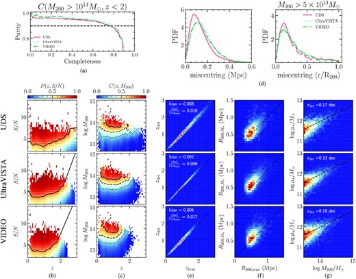
Overview of detectifz selection function using several metrics. (a) Purity versus Completeness for galaxy clusters at z < 2 in the three survey regions (solid red line for UDS, blue dashed line for UltraVISTA and green dash–dotted line for VIDEO). (b) Purity P(z, S/N) as a function of redshift and S/N. The raw two-dimensional histogram is computed in bins of size Δz = 0.05 and ΔS/N = 0.75, but was smoothed with a Gaussian kernel of width σz = 0.25 and σS/N = 0.8 for display purposes. The black solid line shows the |${\rm (S/N)}_{75}(z) \equiv P(z,{\rm S/N}) = 75{{\ \rm per\ cent}}$| threshold (see the text for details). (c) Completeness C(z, MH) as a function of redshift and halo mass M200, with the |${\rm (S/N)}_{75}(z)$| cut applied that ensures a sample purity |$\gt 90{{\ \rm per\ cent}}$|. The raw two-dimensional histogram is computed in bins of size Δz = 0.05 and Δlog M200 = 0.08, but was smoothed with a Gaussian kernel of width σz = 0.25 and |$\sigma _{\log M_{200}} = 0.20$| for display purposes. Solid, dashed, and dotted line show the 75, 50, and 25|${{\ \rm per\ cent}}$| completeness limit, respectively. (d) Distribution of group miscentring in Mpc for all matched groups (left) and in units of r/R200 for matched groups more massive than 1013.5M⊙ (right). (e) Redshift estimated by detectifz zdet versus halo redshift ztrue for matched groups. The bias and scatter is indicated on the top left for each survey region. The dashed line shows the one-to-one line. (f) Estimated group radius |$R_{200, M_\star }$| versus true group radius R200, true. The dashed line shows the one-to-one line. (g) Estimated total stellar mass log μ⋆ versus halo mass log M200. The dashed line shows the best linear fit to the log–log relation. The scatter around the best-fitting relation σdet is shown on the top left.
P(z, S/N) is shown in Fig. 2(b). The purity is an increasing function of S/N at all redshift (higher S/N imply higher purity), and shows a dependence with redshift that makes higher S/N detections having a higher probability to be false detections at higher redshift. This can partially be explained by the fact our stellar-mass cut starts to increase at redshifts where the stellar-mass completeness kicks in (see Section 3.1.1). This behaviour motivated us to define a redshift-dependent S/N cut in order to select a sample with high purity that we will use in the rest of the paper. This cut, |${\rm (S/N)}_{75}(z)$|, is chosen as the S/N at which the purity is |$75{{\ \rm per\ cent}}$| at each redshift. Using this cut, we select a sample that is |$\ge 90{{\ \rm per\ cent}}$| pure at all redshifts.
In Fig. 2(c), we show the completeness C(z, M200) with the |$(S/N)_{75}(z)$| cut in purity applied. This means the completeness we show is for a sample that is |$\gt 90{{\ \rm per\ cent}}$| pure at all redshift. For galaxy clusters (M200 > 1014M⊙), the completeness is |$83{{\ \rm per\ cent}}, 84{{\ \rm per\ cent}}$| and |$78{{\ \rm per\ cent}}$| at z < 2 for UDS, UltraVISTA and VIDEO, respectively. For intermediate mass groups (5 × 10¹³M⊙ < M200 ≤ 1014M⊙), it is |$\sim \! 65{{\ \rm per\ cent}}$| at redshift z < 1 in all three fields and |$65{{\ \rm per\ cent}}, 60{{\ \rm per\ cent}}$| and |$53{{\ \rm per\ cent}}$| for UDS, UltraVISTA and VIDEO respectively at redshift 1 < z < 2. This differences between the three fields is a direct consequence of the different depth (in terms of observed flux) of the three fields. In this range of halo mass, the completeness at 2 < z < 3 is |$23{{\ \rm per\ cent}}$| in UDS and |$16{{\ \rm per\ cent}}$| in UltraVISTA, while there are no detections at these redshifts in VIDEO.
Using our detected groups that are matched to true haloes, we compute statistics about our estimate of group properties. Fig. 2(d) shows the distribution of group miscentring, defined as the distance between detectifz centre and halo centre on the sky, in Mpc (left) and in units of r/R200 (right). We find that |$75{{\ \rm per\ cent}}$| of detectifz groups are miscentred by less than 185, 215, and 220 kpc for UDS, UltraVISTA, and VIDEO, respectively. If looking at groups with M200 > 5 × 10¹³M⊙, |$75{{\ \rm per\ cent}}$| of detectifz are miscentred by less than 0.35 × R200 for all three fields.
In Fig. 2(e), we show the distribution of detected redshifts versus true redshifts. The redshift recovered by detectifz has a very small bias <0.009 overall, and <0.005 at redshift z < 1.5. The median scatter |ztrue − zdet|/(1 + ztrue) is 0.018, 0.006, and 0.017 in UDS, UltraVISTA, and VIDEO, respectively, i.e. half the typical uncertainty on the redshift of individual galaxies.
In Fig. 2(f), we show the distribution of our estimate of the group radius |$R_{200,M_\star }$| versus the true R200 of haloes (estimated from the dark matter density contrast). Our estimate is slightly overestimated by |$11{{\ \rm per\ cent}}, 10{{\ \rm per\ cent}}$| and |$7{{\ \rm per\ cent}}$| for groups with mass 5 × 10¹³M⊙ < M200 < 2 × 10¹⁴M⊙ within the UDS, UltraVISTA, and VIDEO fields, respectively. At M200 > 2 × 10¹⁴M⊙, this bias falls to |$1{{\ \rm per\ cent}}, 2{{\ \rm per\ cent}}$| and |$0.5{{\ \rm per\ cent}}$| within the UDS, UltraVISTA, and VIDEO fields, respectively. The typical scatter on the estimate is ∼0.15 Mpc at all group mass.
Finally, Fig. 2(g) shows the distribution of our mass proxy log μ⋆ formed by summing the stellar masses of galaxies in |$R_{200,M_\star }$|, weighted by their probability of memberships Pmem (see Section 3.7). This estimator is well correlated with halo mass M200. We fit the relation between both variables using a linear model in log–log space using only haloes with mass M200 > 1013.5. The median measured scatter around the best-fitting relation is σmeas = 0.16, 0.15, and 0.16 dex for UDS, UltraVISTA, and VIDEO, respectively. As argued in Euclid Collaboration (2019), to compare different mass proxies that scale differently with halo mass and to account for the intrinsic scatter in the total stellar mass versus halo mass relation, one can form the quantity |$\sigma _{\rm det} = \sqrt{\sigma _{\rm meas}^2/s_{\rm meas}^2 - \sigma _{\rm int}^2/s_{\rm int}^2}$|, which is the scatter due to the detection process. This equation is such that σint is the intrinsic scatter, and |$s_{\rm meas}^2$| and |$s_{\rm int}^2$| are the slopes of the scaling relations for the measured total stellar mass and true total stellar mass, respectively. Using this we find σdet = 0.17, 0.13, and 0.19, respectively. In particular, for groups with mass M200 > 1014M⊙ and z < 2, we find σdet = 0.16 dex for the UDS field, a value directly comparable to the ones given in table 2 of Euclid Collaboration (2019) and which are competitive with the best richness estimates they presented.
The results presented in the previous paragraph show that globally, summing our membership probabilities gives a good mass proxy. To have a more detailed view, we can verify how accurate our probability of membership Pmem is for individual galaxies by comparing it to the fraction of true group members. Only members of groups matched to a true halo and located at a distance less than R200, true of the cluster centre are used in the analysis. In Fig 3, we show the fraction of galaxies that are true cluster members in bins of Pmem for each survey region. We find an overall good agreement, with a deviation of less than |$10{{\ \rm per\ cent}}$| in all bins, showing the strength of our probabilistic membership assignment.
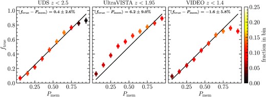
Fraction of true members ftrue versus the estimated probability of membership Pmem for galaxies more massive than 1010.25M⊙ in groups that were match to a halo with mass M200 > 5 × 10¹³ M⊙. For each matched group, only galaxies located in the matched halo projected R200 are considered. Only groups at redshifts z < 2.5 where the 90 per cent stellar-mass completeness limit is greater than 1010.25 M⊙ are considered i.e. z < 2.5 for UDS, z < 1.95 for UltraVISTA and z < 1.4 for VIDEO. The bias, taken as the median ftrue − Pmem weighted by the number of galaxies in each bin of Pmem is shown on the top right.
4.2 The REFINE group catalogue
We applied the detectifz algorithm to the UDS, COSMOS/UltraVISTA, and CFHTLS-D1/VIDEO survey regions. We detect, respectively, 540, 1495, and 553 candidate groups and clusters at S/N > 1.5. We have shown in Section 4.1 that it is necessary to apply a stricter cut in S/N to lower the false detection rate (higher purity). For the remaining of the paper, we use a very strict |$(S/N)_{75}(z)$| that guarantees |$75{{\ \rm per\ cent}}$| purity for clusters with |${\rm S/N} = {\rm (S/N)}_{75}(z)$| at all redshift as illustrated in Fig. 2(b). With this cut, the mean purity is |$\gt 90{{\ \rm per\ cent}}$| at all redshifts. While this impacts the completeness of the sample, high purity is preferred for our study of the group galaxy quenched fraction in Section 5. The estimated completeness as a function of redshift z and halo mass M200 is shown in Fig. 2(c). At this high purity, we have a sample of 448 galaxy groups up to z = 2.5 (77 in UDS, 255 in UltraVISTA and 116 in VIDEO) with 53 groups at z > 1.5 (14 in UDS, 30 in UltraVISTA and 9 in VIDEO).
The redshift, S/N and μ⋆ distributions of our group samples in each of the three survey regions and for the three survey regions combined (REFINE) are shown in Fig 4. Dashed lines show the distributions considering the full sample (S/N > 1.5, completeness |$\gt 90{{\ \rm per\ cent}}$| and purity |$\sim \! 55{{\ \rm per\ cent}}$|), the solid lines show the distributions for the pure sample (|${\rm S/N }\gt {\rm (S/N)}_{75}(z)$|, completeness |$\sim \! 80{{\ \rm per\ cent}}$| and purity |$\gt 90{{\ \rm per\ cent}}$|). Three colour iJK images and some properties of probable group members for three groups at different redshifts in the UDS survey region are presented in Appendix A.
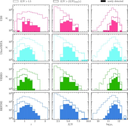
Left: Histogram of redshifts of REFINE candidate groups. Middle: Histogram of S/N of REFINE candidate groups. Right: Histogram of total stellar mass log μ⋆ of REFINE groups. From top to bottom the rows display the UDS, UltraVISTA, VIDEO, and REFINE (UDS + UltraVISTA + VIDEO) survey. We show the distributions of all candidate groups (S/N > 1.5, dashed line), |$90{{\ \rm per\ cent}}$| pure group sample (|${\rm S/N} \gt {\rm (S/N)}_{75}(z)$|, solid line) and the newly discovered groups (filled histogram).
4.3 Comparison to existing cluster catalogues
To further assess the quality of our group sample and quantify which of our detections are new, we compared our group catalogues to the literature. In the three survey regions considered in this work, many previous studies have tackled group or cluster detection, in a variety of redshift ranges, using either optical and near-infrared data or X-ray data.
To match our clusters to other catalogues, we used two-way geometrical matching (see Euclid Collaboration 2019), considering two detections are matched if they are at a distance d < 1 Mpc on the sky (at the redshift of the detectifz group) and |$\vert \Delta z \vert \lt 2\times \langle \sigma _z^{68}\rangle _{P_{68}}(z)$|. As catalogues from the literature have different completeness and purity level, we cannot properly assess our own completeness and purity from comparison to these. Yet for any given catalogue from the literature, we compute the percentage of their clusters located in the same field as ours that we detect at S/N > 1.5 (that we call re-detected groups) and the number of detectifz secure detections (|${\rm S/N} \gt {\rm (S/N)}_{75}(z)$|) that are not detected in other surveys (that we call newly detected groups). Overall, in our pure sample, we find 170 newly detected galaxy groups (31 in UDS, 91 in UltraVISTA and 48 in VIDEO). At z > 1.5, 38 groups of our pure sample are newly detected (11 in UDS, 19 in UltraVISTA and 8 in VIDEO). Properties of the newly detected clusters for the full REFINE survey are shown in the bottom row of Fig. 4 as filled histograms. We discuss these newly detected clusters in the subsections below.
4.3.1 UDS
In the UDS field, we matched our group catalogue to public catalogues from the literature. Lee et al. (2015b), Socolovsky et al. (2018), and Galametz et al. (2018) detected 46, 39, and 34 galaxy group and clusters in the UDS field of view using data from the UDS survey in the redshift range 0.5 < z < 2, 0.5 < z < 1, and 0.6 < z < 0.7, respectively. The UDS field is also located inside several other surveys in which clusters and groups were detected. We list them here with the redshift ranges of the clusters. In the W1 field of the CFHTLS survey, we used catalogues from Ford et al. (2015) (118 clusters at 0.2 < z < 1 in UDS), Licitra et al. (2016) (3 clusters at 0.45 < z < 0.79 in UDS), and Sarron et al. (2018) (5 clusters at 0.53 < z < 0.7 in UDS). In the HSC-SSPxunWISE survey, we used the catalogue of Wen & Han (2021) (12 clusters at 0.40 < z < 1.43 in UDS). In the X-rays, we used the catalogues of Finoguenov et al. (2010) (43 clusters at 0.19 < z < 2.15 in UDS) from the Subaru-XMM Deep Field (SXDF) and Adami et al. (2018) (10 clusters at 0.18 < z < 1.1 in UDS) from the XXL survey.
Results from matching these catalogues to ours are summarized in Table 1, and are shown in the first row of Fig. 4 as filled histograms. We also present a comparison between our group mass proxy μ⋆ and those of other catalogues in online Appendix D.
The number (Nmatch) of groups in catalogues from the literature also detected by detectifz, and the percentage of the original catalogue re-detected in the UDS field.
The number (Nmatch) of groups in catalogues from the literature also detected by detectifz, and the percentage of the original catalogue re-detected in the UDS field.
4.3.2 COSMOS/UltraVISTA
In the UltraVISTA field, we matched our group catalogue to six public catalogues from the literature obtained from optical and X-ray data. In the optical, Bellagamba et al. (2011) detected 142 clusters in the redshift range 0.12 < z < 0.8 in the UltraVISTA survey region, while Wen & Han (2011) detected 209 clusters in the redshift range 0.17 < z < 1.61. Chiang et al. (2014) looked for overdensities of galaxies based on photometric redshifts at z > 1.5 on scales of ∼15 Mpc. They detected 36 such overdensities in the range 1.6 < z < 3.09. Recently, Ando et al. (2020) looked for protocluster cores at z > 1.5 using galaxy photometric redshifts. They detected 75 protocluster cores in the range 1.5 < z < 2.93. Wen & Han (2021) looked for galaxy clusters in the HSC-SSPxunWISE field, using optical and near-infrared data. In the area of the COSMOS/UltraVISTA, they detected 69 galaxy clusters in the redshift range 0.2 < z < 1.51. In the X-rays, Gozaliasl et al. (2019) detected 230 galaxy clusters in the COSMOS/UltraVISTA field at redshift 0.05 < z < 1.53.
Results from matching these catalogues to ours are summarized in Table 2, and are shown in the second row of Fig. 4 as filled histograms. We also present a comparison between our group mass proxy μ⋆ and those of other catalogues in online Appendix D.
The number (Nmatch) of groups in catalogues from the literature also detected by detectifz, and the percentage of the original catalogue re-detected in the COSMOS/UltraVISTA field.
The number (Nmatch) of groups in catalogues from the literature also detected by detectifz, and the percentage of the original catalogue re-detected in the COSMOS/UltraVISTA field.
4.3.3 CFHTLS-D1/VIDEO
In the VIDEO field, we matched our group catalogue to seven public catalogues from the literature obtained from optical and X-ray data in different survey areas. As this field is located in the W1 field of the CFHTLS, as for UDS we used the catalogues of Ford et al. (2015) (152 clusters at 0.2 < z < 1.01 in CFHTLS-D1), Licitra et al. (2016) (15 clusters at 0.14 < z < 1.02 in CFHTLS-D1), and Sarron et al. (2018) (6 clusters at 0.18 < z < 0.53 in CFHTLS-D1). In the HSC-SSPxunWISE survey, we used the catalogue of Wen & Han (2021) (27 clusters at 0.25 < z < 1.53 in CFHTLS-D1). In the X-rays, we used the catalogue of Gozaliasl et al. (2014) (42 clusters at 0.14 < z < 1.08 in CFHTLS-D1) and two catalogues from the XXL survey, Adami et al. (2018) (10 clusters at 0.04 < z < 1.06 in CFHTLS-D1) and Trudeau et al. (2020) that detected high redshift XXL clusters counterparts in the optical/near-infrared (8 clusters at 0.82 < z < 1.94 in CFHTLS-D1).
Results from matching these catalogues to ours are summarized in Table 3 and shown in the third row of Fig. 4 as filled histograms. We also present a comparison between our group mass proxy μ⋆ and those of other catalogues in online Appendix D.
The number (Nmatch) of groups in catalogues from the literature also detected by detectifz, and percentage of the original catalogue re-detected in the CFHTLS-D1/VIDEO field.
The number (Nmatch) of groups in catalogues from the literature also detected by detectifz, and percentage of the original catalogue re-detected in the CFHTLS-D1/VIDEO field.
5 QUENCHED FRACTIONS
This section is dedicated to a preliminary study of the cluster/group galaxy quenched fraction in our candidate cluster/group sample. We voluntarily limit ourselves here to the study of galaxies with stellar masses 1010.25 < M⋆/M⊙ < 1011 and within 0.5 × R200 the group centre, in groups with total stellar mass log μ⋆ > 11.25. The lower stellar mass limit ensures |$90{{\ \rm per\ cent}}$| stellar-mass completeness for all groups. Using these cuts, we are left with 403 galaxy groups in the range 0.12 ≤ z < 2.32 for which the estimated purity is |$\gt 90{{\ \rm per\ cent}}$|. The upper mass limit removes the contribution of massive galaxies for which mass quenching is thought to be the dominant quenching process. It also allows us to remove the relative excess of these galaxies in groups compared to the field that would prevent any interpretation of the results in terms of the effect of the environment. Overall, we checked that using this mass range ensures that we are comparing samples with similar stellar-mass distributions and mean galaxy stellar mass M⋆ ∼ 1010.6M⊙ in the groups and M⋆ ∼ 1010.55M⊙ in the field. The radial limit means that we are only probing the group core that is characterized by a higher density contrast. Doing this makes it easier to isolate the effect of the group on the quenching fraction. Further investigation of the stellar-mass and radial dependence through computation of group galaxy stellar mass function (GSMF) and radial distributions, respectively, will be presented in a future work.
5.1 Number counts
To compute the group galaxy quenched fraction, we first compute the galaxy number counts for all galaxies and quenched galaxies in groups and outside groups (field), respectively. When considering galaxies at all sSFR values, number counts are computed using the method introduced Section 2.2 with appropriate binning in redshift and stellar mass.
5.2 Bayesian model
From these distributions, we then compute |$f^q_{\rm group}$|, the posterior for the quenched fraction of group galaxies considering we observed the sum of the two populations. We take uniform (flat) priors for all parameters (see online Appendix E for details). MCMC sampling of this model is performed using the PYMC3 python package.
5.3 Fraction of quenched galaxies in individual groups
The fraction of quenched galaxies can then be computed for each individual galaxy group using the number counts and the Bayesian model presented in the two previous subsection. In practice, for each group, we need the total (group+field) counts and total quenched counts in the cluster region and reference counts from the fields. For the reference counts, as we want to use the group sample to infer properties of groups in general, we need to ensure that these counts are independent for each group, in order not to overestimate the strength of our results (see Raichoor & Andreon 2012). To this aim, at each redshift step dz = 0.01, we remove galaxies closer than 2 × R200 from groups that may contribute to this redshift (whose PDFgroup(z) > 0 at this redshift). Remaining galaxies are considered field galaxies at this redshift z. To keep independent counts for each group we use galaxies outside of our groups at each group’s best redshift zgroup, and located in an annulus between 3 Mpc and 5 Mpc from the group centre. Using counts near the location of the group (local field) has the double advantage of ensuring independence of each group as well as accounting for correlated structures in the group vicinity.
5.4 Stacking in redshift bins
To better understand the redshift evolution of the group quenched fraction |$f_{\rm group}^q$|, and compare the three survey regions, we stack individual groups in redshift bins. In our Bayesian inference framework, this comes to consider each individual group as one observation of the true underlying population in the redshift bin.
For each of the three survey regions, we bin groups in 6 redshift bins. These bins were chosen to be roughly equally populated. The highest redshift bin is slightly different between UDS and UltraVISTA. This is due to the UltraVISTA stellar-mass completeness reaching 1010.25M⊙ at redshift z = 1.95. For the same reason, there are no groups in the highest redshift bins for the VIDEO survey region. We have about 10, 40 and 15 groups per bin in the UDS, UltraVISTA and VIDEO regions respectively using this binning. The quenched fraction obtained are presented in Table 4 and Fig. 5
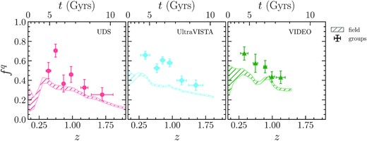
Quenched fraction for galaxies with stellar-mass 1010.25 < M⋆/M⊙ < 11 in detectifz groups at r < 0.5 × R200. From left to right are shown the UDS (red dots), UltraVISTA (blue diamonds), and VIDEO (green triangles) survey regions. The point with error bar show the group quenched fraction in the redshift bins defined in Table 4. Points are located at the median redshift of the bin and horizontal errorbars show the standard deviation of the redshift distributions of groups in the bin. Vertical errorbars are 68 per cent confidence limits in the |$f_{\rm group}^q$| value. The dashed region shows the |$68{{\ \rm per\ cent}}$| confidence region for the field quenched fraction |$f^q_{\rm field}$|.
Quenched fraction in redshift bins.
| redshift range | 〈z〉median | |$f_{\rm group}^q$| | Ngroup |
|---|---|---|---|
| UDS | |||
| 0.12 ≤ z < 0.52 | 0.46 | |$0.497^{+0.086}_{-0.080}$| | 11 |
| 0.52 ≤ z < 0.73 | 0.62 | |$0.705^{+0.066}_{-0.067}$| | 10 |
| 0.73 ≤ z < 0.88 | 0.8 | |$0.365^{+0.090}_{-0.085}$| | 11 |
| 0.88 ≤ z < 1.08 | 0.97 | |$0.460^{+0.082}_{-0.081}$| | 10 |
| 1.08 ≤ z < 1.42 | 1.27 | |$0.325^{+0.084}_{-0.078}$| | 9 |
| 1.42 ≤ z < 2.32 | 1.66 | |$0.253^{+0.072}_{-0.063}$| | 16 |
| UltraVISTA | |||
| 0.12 ≤ z < 0.52 | 0.39 | |$0.658^{+0.041}_{-0.043}$| | 39 |
| 0.52 ≤ z < 0.73 | 0.65 | |$0.525^{+0.046}_{-0.046}$| | 41 |
| 0.73 ≤ z < 0.88 | 0.78 | |$0.606^{+0.038}_{-0.038}$| | 41 |
| 0.88 ≤ z < 1.08 | 0.94 | |$0.579^{+0.040}_{-0.041}$| | 40 |
| 1.08 ≤ z < 1.42 | 1.21 | |$0.399^{+0.045}_{-0.043}$| | 43 |
| 1.42 ≤ z < 1.95 | 1.53 | |$0.349^{+0.054}_{-0.052}$| | 38 |
| VIDEO | |||
| 0.12 ≤ z < 0.52 | 0.37 | |$0.677^{+0.067}_{-0.070}$| | 16 |
| 0.52 ≤ z < 0.73 | 0.62 | |$0.575^{+0.093}_{-0.094}$| | 15 |
| 0.73 ≤ z < 0.88 | 0.84 | |$0.541^{+0.062}_{-0.064}$| | 15 |
| 0.88 ≤ z < 1.08 | 0.99 | |$0.437^{+0.052}_{-0.052}$| | 25 |
| 1.08 ≤ z < 1.42 | 1.16 | |$0.430^{+0.066}_{-0.064}$| | 20 |
First, we note that the quenched fractions in the field and their redshift evolution are comparable in the three survey regions with an offset of ∼0.05. We verified that the distribution in log SFR versus log M⋆ are similar for the three survey regions, as well as the normalization and slope of the star-forming main sequence. We also verified that the offsets are not significant when accounting for cosmic variance using the GETCV IDL routine of Moster et al. (2011).
In the entire redshift range probed here (0.12 ≤ z < 2.32) and each of the three surveys, the quenched fractions in the groups are found to be higher than in the field. However, due to the relatively small number of groups in each bin this trend is not very significant in some redshift bins in the UDS and VIDEO fields. Moreover, the group quenched fraction in redshift bins is similar between the different survey regions, with differences always smaller than 2.5σ (∼1σ in the mean). Considering the two previous points, we now study the group quenched fraction evolution jointly for the full REFINE survey.
5.5 Quenched fraction redshift evolution in REFINE
In addition to this hierarchical fit, we also computed the group quenched fraction in 13 equipopulated bins to allow for a sanity check of the goodness of fit. With this binning, we have ∼30 groups per bins. Results are presented in the left panel of Fig. 6. The group quenched fraction in our REFINE group sample is compatible with a linear decreasing redshift evolution, with |$\alpha _z = -1.11^{+0.15}_{-0.16}$| and f1 = −0.07 ± 0.06. The group quenched fraction of our REFINE group sample is found to be significantly higher than the field quenched fraction with higher confidence at low redshift. The confidence of the result monotonically drops with increasing redshift reaching 3σ, 2σ and 1σ confidences at redshift z = 1.55, 1.79 and 2.23 respectively. These results are discussed and compared to the literature in Section 6.2. We note that when running a similar hierarchical model (not presented here) for the global field quenched fraction on the REFINE sample, we also find it is compatible with a linear decreasing redshift evolution.
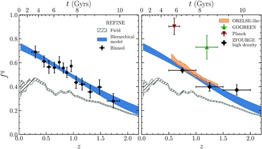
Quenched fraction for galaxies with stellar-mass 1010.25 < M⋆/M⊙ < 11 in detectifz groups at r < 0.5 × R200. Left: shows results for the full REFINE data. Points with errorbars show the binned group quenched fraction |$f_{\rm group}^q$|. Points are located at the median redshift of the bin, and the horizontal errorbars show the standard deviation of the redshift distributions of groups in the bin. Vertical errorbars are 68 per cent confidence limits in the |$f_{\rm group}^q$| value. The shaded region displays the |$68{{\ \rm per\ cent}}$| confidence interval on |$f_{\rm group}^q(z)$| for the hierarchical model defined in equation (19). The dashed region shows the |$68{{\ \rm per\ cent}}$| confidence region for the field quenched fraction |$f^q_{\rm field}$|. Right: |$f^q_{\rm field}$| and |$f_{\rm group}^q(z)$| from the left panel are reported and compared to values taken from the literature (ZFOURGE, ORELSE, Planck clusters, and GOGREEN). See the text for details.
5.6 QFE in REFINE
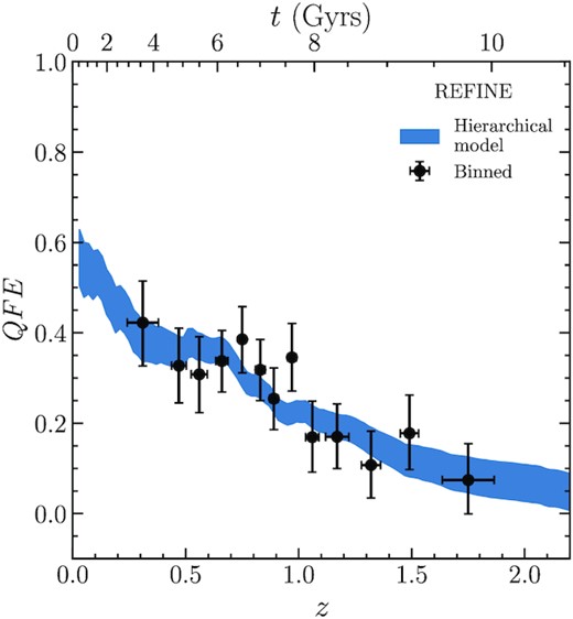
QFE for galaxies with stellar-mass 1010.25 < M⋆/M⊙ < 11 in detectifz groups at r < 0.5 × R200. Points with errorbars shows the binned group quenched fraction (QFE). Points are located at the median redshift of the bin and horizontal errorbars show the standard deviation of the redshift distributions of groups in the bin. Vertical errorbars are 68 per cent confidence limits in the QFE value. The shaded region shows the |$68{{\ \rm per\ cent}}$| confidence interval on QFE(z) obtained using |$f^q_{\rm group}(z)$| from the hierarchical model defined in equation (19).
6 DISCUSSION
6.1 Quenched and star-forming galaxies: sSFR cut
We note that across the literature, many different cuts are used to select star-forming versus quenched galaxies (e.g. red-sequence: Popesso et al. 2006, SED fitting based classification: Sarron et al. 2018 or observed colour–colour: Bisigello et al. 2020). A selection criterion that has gained in popularity is a rest-frame colour–colour cut based on the UVJ diagram first proposed by Williams et al. (2009) and then expended by other works using slightly different filters (NUVrK; Arnouts et al. 2013).
In this work, we decided to use a cut in specific star formation rate (sSFR) estimated from template fitting. We chose this selection criteria because in our probabilistic approach, it allows us to compute a probability that each galaxy is quenched at a given redshift (see Section 5.1). This way, our approach makes the quenched versus star-forming binary classification less strict and more resilient in degenerate cases.
We note that it has been showed that SED fitting SFR estimates are in general noisier and more biased than NUVrK SFR estimates (see Lee et al. 2015a). However, the discrepancy between both methods (bias) concerns mainly star-forming galaxies with SFR > 101.5M⊙yr−1 which should not affect much the quenched versus star-forming binary classification. Moreover, with our probabilistic approach this possible mis-classification due to the higher scatter in SED fitting SFR estimates is mitigated.
In practice, we computed the probability for each galaxy to be quenched at each redshift, using a constant cut in sSFR (sSFR<10−11yr−1). Ilbert et al. (2013) showed that such a cut is similar to their colour–colour cut NUV − r+ versus r+ − J at z < 1 and more conservative at z > 1. A similar trend was found in Ilbert et al. (2015) who found a sSFR<10−11yr−1 cut was very close to a colour–colour cut in NUV − R versus R − K out to z = 1.4. We however investigate alternative constant cuts and find very similar results to what follows. Some authors (e.g. Lee et al. 2015b; Jian et al. 2018) use instead a sSFR cut that evolves with redshift, to account for the general evolution of the galaxy star-forming main-sequence with redshift. However Lee et al. (2015b) showed that this redshift dependent cut, even though it yields different quenched fraction values (higher at high redshift) does not affect the general trend of their results with galaxy stellar mass and environment. We investigated this and find largely the same result.
6.2 Quenched fraction: Comparison to previous studies
A number of studies computed the quenched fraction fq at different redshifts and stellar masses in different environments. Here, we are interested in comparing our results with studies looking at similar redshifts and stellar masses in high-density environments, in particular at z > 1. We focus on the results presented in Papovich et al. (2018) at 0.15 < z < 2.0 in the ZFOURGE survey (Straatman et al. 2016), Lemaux et al. (2019) at 0.55 < z < 1.4 in the ORELSE survey (Lubin et al. 2009), van der Burg et al. (2018) at 0.5 < z < 0.7 using Planck detected clusters and van der Burg et al. (2020) at 1.0 < z < 1.4 in the GOGREEN survey (Balogh et al. 2017) as they provide either the GSMF (ZFOURGE, Planck clusters, and GOGREEN) or an analytical fit to the quenched fraction as a function of redshift, stellar mass and overdensity level (ORELSE), that allows for a fair comparison of our results to theirs (in particular using the same stellar-mass limits).
To probe the effect of environment on galaxy star formation at high redshift, different approaches have been used in the literature. A common approach in deep contiguous surveys is to split the density field in four quartiles (e.g. ZFOURGE; Papovich et al. 2018). On the other hand, one can instead observe some massive candidate galaxy clusters at different locations in the sky using dedicated observations (e.g. GOGREEN; van der Burg et al. 2020). The ORELSE survey took a hybrid approach, targeting specifically regions around massive clusters and studying regions with different overdensities in these fields (Lemaux et al. 2019).
Our own approach consists in detecting candidate groups in contiguous survey regions. Compared to a simple density cut, our method allows us to detect specifically structures that correspond to dark matter haloes, rather than galaxy filaments for example, that may be included in the highest density quartile of ZFOURGE. Owing to the relatively small volume covered by our three survey regions, our probability of observing massive clusters is low and we in fact do not observe very rich structures, contrary to the GOGREEN and ORELSE survey. Our study thus targets intermediate mass groups (at 0.12 ≤ z < 2.32), a mass regime that is targeted by ORELSE (at 0.55 < z < 1.4) but not by ZFOURGE, Planck, and GOGREEN.
Comparison of our quenched fractions fq with those of the four works mentioned earlier are presented in the right panel of Fig. 6. For ZFOURGE, Planck clusters and GOGREEN, quenched fractions are obtained using the empirical binned GSMF of the quenched and total galaxy population provided in each study. While the raw data is provided for Planck and GOGREEN, for ZFOURGE we extracted values of the data points from their figures using the WebPlotDigitizer tool (Rohatgi 2020). The quenched fraction fq is taken as the ratio of the quenched and total GSFM summed in the range 10.25 < log M⋆/M⊙ < 11. For the ORELSE survey, we use the fit provided in Papovich et al. (2018) that gives fq as a function of redshift, stellar mass and overdensity log (1 + δgal). In each of the redshift bins used for the REFINE survey (showed in the left-hand panel of Fig. 6) that fall in the range 0.55 < z < 1.4, we compute the median stellar mass (∼1010.60M⊙) and |$68{{\ \rm per\ cent}}$| interval of overdensity |$\log (1+\delta _{M_\star })$| in 0.5R200 using the detectifz density maps. Under the approximation |$\delta _{M_\star } \simeq \delta _{\rm gal}$|, this allow us to obtain an estimate of our sample quenched fraction using the ORELSE parametrization that we now refer to as the ORELSE-like quenched fraction.
We find a very good agreement between our quenched fraction estimate and that of ZFOURGE and ORELSE-like. It should be noted that the ZFOURGE estimate at 1.5 < z < 2 is ∼0.1 higher than ours (0.37 ± 0.04 versus 0.28 ± 0.03, 1.7σ discrepancy). This discrepancy may come from different overdensities probed in this bin between ZFOURGE and our sample. We find that the ORELSE-like estimates are slightly higher than ours. The quenched fraction estimates however never differ by more than 1.3σ and around 0.5σ in the central part of the redshift ranged probed by the ORELSE survey. The slightly higher estimate for ORELSE-like parametrization could also be due to the fact that the quenched fraction estimates at M⋆ < 1010.5 (about half the weight of our sample) should be considered upper limits according to Papovich et al. (2018).
This relatively good agreement is particularly remarkable as ZFOURGE, ORELSE, and our work used different cuts to segregate quenched and star-forming galaxies. This strengthens the argument made in Section 6.1 that our probabilistic sSFR<10−11yr−1 cut is effectively equivalent to colour–colour cuts in UVJ (ZFOURGE) and NUVrJ (ORELSE), respectively.
On the other hand, there is a large discrepancy between our quenched fractions and those of van der Burg et al. (2018, 2020) at redshift 0.5 < z < 0.7 and 1.0 < z < 1.4, respectively. Quenched fraction of the Planck clusters are 0.31 higher than ours (0.90 ± 0.07 versus 0.59 ± 0.01, 4.4σ discrepancy). Quenched fraction of the GOGREEN clusters are also ∼0.30 higher than ours (0.73 ± 0.10 versus 0.43 ± 0.02, a 3σ discrepancy). To investigate the origin of this difference, for the GOGREEN survey, we use the cluster richness provided in van der Burg et al. (2020). Using the van der Burg et al. (2020) definition of richness, our sample in 1.0 < z < 1.4 has a median richness of 9.5, while GOGREEN clusters have a median richness of 35.8. For the Planck cluster sample, van der Burg et al. (2018) do not provide a richness estimate that we can compare to ours. However, their clusters have estimated masses M500 > 5 × 10¹⁴M⊙. Following the mass-richness scaling we found in our mock data, these massive clusters probe a very different halo mass range compared to our sample that is expected to be populated mostly with intermediate mass groups (M200 ∼ 5 × 10¹³M⊙).
The galaxy quenched fraction is known to depend on cluster mass up to at least z = 0.7 (Sarron et al. 2018), with higher mass clusters having higher quenched fractions. While it is still unsure whether this result holds at higher redshift, it would explain our lower quenched fractions compared to van der Burg et al. (2018, 2020).
6.3 QFE: redshift evolution
We observe a decrease of the QFE as a function of increasing redshift from QFE = 0.53 at z = 0.12 to QFE = 0.035 at z = 2.31 (respectively the lowest and highest redshifts of groups used in this work). In order to interpret this result in terms of efficiency of quenching in galaxy groups, we need to ensure that we are comparing similar galaxy groups/overdensities at different redshifts and galaxies of similar stellar masses. We note that, adopting this strategy, we are in fact looking at environments that are similar at different redshifts, thus not addressing the question of mass accretion on to haloes i.e. our high redshift groups are not the progenitors of our low redshift groups. The same is true for galaxies. We postpone such an analysis using the REFINE detectifz group sample to future work.
To check that we probe similar environments at all redshift, we verified that in the redshift bins showed in Fig. 6, the groups have the same range of total stellar mass. We further checked that the typical |$\delta _{M_\star }$| in 0.5 × R200 is not redshift dependent. It is in fact constant around |$\log (1 + \delta _{M_\star }) \sim 1 \pm 0.2$| (SD) in the range 0.12 < z < 2.32.
To check that we study galaxies of similar stellar masses at different redshift, we verified that, in the redshift bins showed in Fig. 6, galaxy stellar masses in the group and field sample have similar distributions and that these distributions are roughly independent of redshift. We find that the median stellar mass is 0.05 dex higher in our groups than in the field overall (1010.6M⊙ versus 1010.55M⊙), but the range covered by |$68{{\ \rm per\ cent}}$| of the distributions are very similar 10.36 < log M⋆/M⊙ < 10.87 versus 10.34 < log M⋆/M⊙ < 10.83. The offset between median stellar masses in the group and field shows a slight redshift evolution from 0.04 at z ∼ 0.5 to 0.09 dex at z ∼ 2, but this shift is not significant considering the spread of the stellar mass distributions.
With the two previous checks, we can exclude that the observed increase of QFE with decreasing redshift is due to observing more overdense groups at low redshift or galaxies of different stellar masses. However, as already mentioned, one needs to keep in mind that due to large-scale accretion (or equivalently halo mass growth) through cosmic time, galaxies in groups at z ∼ 2 and z ∼ 0.5 may have lived in different environments before entering the group. Indeed, the density contrast of the universe increases with cosmic time. This implies that galaxies in groups at lower redshift are expected to have spent more time in denser cosmic filaments than galaxies in groups at high redshift. Cosmic filaments have been shown to have higher quenched fraction than the field up to z = 0.9 (see e.g. Martínez, Muriel & Coenda 2016; Salerno, Martínez & Muriel 2019; Sarron et al. 2019) and to they play a specific role in quenching (see Laigle et al. 2018; Kraljic et al. 2018). Thus, without quantifying properly the level of pre-processing by cosmic filaments and its redshift evolution, we cannot conclude that the observed increase of QFE with decreasing redshift is due to a specific quenching mechanism in the group environment whose efficiency might change with redshift. Computing the GSMF and radial distribution of quenched and star-forming galaxies should allow to address these points in more details (see e.g. van der Burg et al. 2018).
7 CONCLUSIONS
In this paper we carry out a detailed investigation of groups and clusters in the three largest and deepest ground based surveys as part of the REFINE survey. Through a reanalysis of the redshifts and stellar masses of the UDS, COSMOS/UltraVISTA and CFHTLS-D1/VIDEO fields we develop a new methodology, called detectifz for finding clusters and groups up to z ∼ 3 within these fields.
To find these distant groups and clusters and determine cluster/group membership, our method uses the joint PDFs for the stellar masses and redshifts of all the galaxies in the REFINE survey. We furthermore extensively test our methodology on simulation mocks which are designed to mimic the properties of the observational data that we use in this study. Using these mocks, we show that we are able to retrieve a large fraction of all overdensities of galaxies and retrieve their properties accurately.
Overall, we detect and measure properties of 2588 candidate galaxy groups and clusters up to z = 3.15 at S/N > 1.5. We build a very pure (|$\gt 90{{\ \rm per\ cent}}$|) sample of 448 candidate groups up to z = 2.5 (out of which 170 are newly detected) and study some of their properties, of which this paper is an initial investigation.
We use these results to investigate the quenched fraction of galaxies as a function of redshift and environment up to z = 2.31. We show that the differences between the quenched fraction in the field and in groups/clusters grows at lower redshifts, such that the differences in quenched fractions reach ∼0.3 at z ∼ 0.1, while it is ∼0.05 at z ∼ 2. As a result, we find that the QFE in groups grows at lower redshift from QFE = 0.035 at z = 2.31 to 0.53 at z = 0.12.
We emphasize that these results are hard to interpret in terms of an increased quenching efficiency of the group environment at lower redshift at fixed halo mass/overdensity due to possible pre-processing happening outside the group environment (cosmic filaments) through cosmic time. We plan to explore this aspect in more details through an analysis of the group galaxy stellar-mass function and radial profile up to several virial radii in future work.
SUPPORTING INFORMATION
Appendix D. Group mass proxy: comparison to literature
Appendix E. Quenched fractions: Priors of Bayesian models
Please note: Oxford University Press is not responsible for the content or functionality of any supporting materials supplied by the authors. Any queries (other than missing material) should be directed to the corresponding author for the article.
ACKNOWLEDGEMENTS
We thank Ulrike Kuchner for useful discussions, and thank the various teams that produced the initial images we use from UltraVISTA, UDS and VIDEO. We also thank the anonymous referee for helping improve the paper readability. This study was supported by a Cosmic Visions STFC grant and by the Universities of Manchester and Nottingham.
DATA AVAILABILITY
The detectifz python package used to detect galaxy groups will be made available at https://github.com/fsarron/detectifz, along with the group and group member catalogues. The group catalogues will also be released at the CDS. The remaining data underlying this article, including galaxy catalogues, mock galaxy catalogues, galaxy physical parameter estimate PDF and their by-products (e.g. galaxy number counts and quenched fractions) will be shared on reasonable request to the corresponding author.
Footnotes
REFERENCES
APPENDIX A: EXAMPLES OF DETECTIFz GROUPS IN THE UDS FIELD
In Fig. A1, we show example iJK images and some properties of galaxies near the identified group centre. The three groups were detected in the UDS survey region at redshifts z = 0.6, 1.28, and 2.20, respectively, at S/N ≥ 5. The iJK images are centred on each detectifz group’s centre. The bottom row shows galaxies in the group field of view at a distance |$d \lt R_{200,M_\star }$| from the group centre and with Pmem > 0.2. The point size is proportional to the galaxy median stellar mass at the group redshift |$M_\star ^{{\rm median},z_{\rm group}} = \langle \int {\rm PDF}_{\rm gal}(M_\star ,z)~{\rm PDF}_{\rm group}(z)~{\rm d}z\rangle _{\rm median}$| and colour-coded with the probability that the galaxy is quenched if located at the group redshift |$\scriptstyle{P^q_{z_{\rm group}} = \int P^q(z)~{\rm PDF}_{\rm group}(z)~{\rm d}z}$|, similarly to the quantities used for delocalized number counts in Section 5.1. We note that the group at z = 1.28 is newly detected by detectifz.
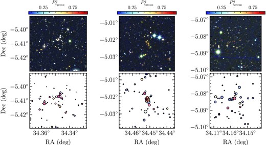
Top row: From left to right, iJK images of three clusters located at z = 0.6, 1.28, and 2.20, respectively. Bottom row: galaxies in the group field of view at a distance |$d \lt R_{200,M_\star }$| from the group centre and with Pmem > 0.2 colour coded by their probability to be quenched at the group redshift. The point size is proportional to the galaxy stellar mass at the group redshift. See the text for details.
APPENDIX B: TECHNICAL DETAILS ON MOCKS
In this appendix, we give the technical details of the method we used to build mock data resembling REFINE data from the lightcones of Henriques et al. (2015) that were briefly presented in Section 2.3.
B0.1 Survey geometry and K-band magnitude
B0.2 The PDF(M⋆, z) and (M⋆, z) shift
We want each mock galaxy to have its redshift and stellar-mass shifted from its true value with a shift typical of what is expected for such a galaxy in the data. Each mock galaxy should also have a PDF(M⋆, z) typical of what is expected for such a galaxy in the data.
To do this, we binned the data in 2D bins |$(M_\star ^{\rm median}, z_{\rm phot})$| with stellar-mass and redshift steps of dM⋆ = 0.05 and dz = 0.01 as for PDF(M⋆, z). To avoid too sparse sampling and because of the typical uncertainty on these points estimates of M⋆ and z, the size of the bins are taken to be |$\Delta M_\star = \langle \sigma ^{68}_{M_\star }\rangle _{\rm median} = 0.2$| and Δz = σ0 × (1 + z), with σ0 = 0.045, 0.01, 0.035 for UDS, UltraVISTA, and VIDEO, respectively, effectively applying a running window with overlapping bins. Similarly, we binned mock galaxies in 2D bins |$(M_\star ^{\rm true}, z^{\rm true})$| with stellar-mass and redshift steps of dM⋆ = ΔM⋆ = 0.05 and dz = Δz = 0.01. Here, the bins are not overlapping as |$M_\star ^{\rm true}$| and ztrue are known exactly.
Each bin (M⋆, z)bin is populated with |$N_{\rm gal,bin}^{\rm data}$| and |$N_{\rm gal,bin}^{\rm mock}$|. We bootstrap |$N_{\rm gal,bin}^{\rm mock}$| from the list of |$N_{\rm gal,bin}^{\rm data}$| data galaxies. This effectively gives us a PDF(M⋆, z) for each of these mock galaxies. We note that some (|$\lt 1{{\ \rm per\ cent}}$|) mock galaxies have |$(M_\star ^{\rm true},z^{\rm true})$| values that do not appear in the data. We assign to these 2D normal PDFs centred at the bin values, with standard deviations |$(\langle \sigma ^{68}_{M_\star }\rangle _{\rm median},\sigma _0 \times (1+z^{\rm true}))$| and no covariance.
Each mock galaxy PDF(M⋆, z) is re-centred at the central value of the bin (M⋆, z)bin. We use the PINKY python package to sample a given |$(\widehat{M}_\star ^{\rm median},\widehat{z}_{\rm phot})$| from the PDF, and re-centre the PDF at these sampled values.
This last PDF(M⋆, z) is our final estimate for the mock galaxies. It is sampled directly from the data and has been shifted to account for the uncertainty information it encompasses.
APPENDIX C: TECHNICAL DETAILS ON THE PROBABILISTIC MEMBERSHIP ASSIGNMENT
C1 Bayesian formalism
As mentioned in Section 3.6, the probabilistic membership of group members is computed in a Bayesian formalism similar to that developed in George et al. (2011) and Castignani & Benoist (2016) in which the probability for a galaxy (gal) to be a member of a given group (G) is defined as the posterior probability Pmem ≡ P(gal ∈ G|PDFgal(M⋆, z), PDFgroup(z)). In all generality, we should adopt a cluster model specifying the group galaxy stellar-mass function (GSMF) and redshift distribution to which the observed PDFgal(M⋆, z) is to be compared. Keeping in line with the detectifz idea of being model free, as models (in particular group GSMF) are not yet well constrained at low group mass and high redshift, we instead reduce constraints on M⋆ by marginalizing it out, and consider only the redshift information PDF(z). The redshift distribution is modelled by the δ distribution in redshift peaked at zgroup. As the photometric redshift uncertainty is an order of magnitude larger than the actual group size in redshift space, this makes a more sophisticated model unnecessary for our purpose.
C2 Likelihood
C3 Prior
The prior probability |$P^{\rm prior}(z\vert M_\star ^{\rm gal}) \equiv P({\rm gal} \in G~\vert ~{\rm PDF}_{\rm group}(z), M_\star)(z)$| is obtained by quantifying the number count excess at the galaxy position for each z. To this aim we first need to compute galaxy number counts at the group redshift zgroup knowing the uncertainty on this value encoded in PDFgroup(z).
There are two additional correction factors in this equation: floc and fsky. The former allows us to correct for the local large-scale structure bias around the cluster that may be higher or lower than the mean field value obtained from the full survey (Fnoclus), similarly to Castignani & Benoist (2016). The latter allows us to account for the cluster profile, giving higher Pprior values to galaxies located in the denser regions of the group. Both are computed using the density maps generated in Section 3.1.3 at the group best redshift zgroup. The value floc is the ratio between the mean pixel value in an annulus centred at the group centre with inner radius 3 Mpc and outer radius 5 Mpc, and the mean pixel value over the all field (with the clusters removed). Furthermore, fsky is the ratio between the value of the pixel in which the galaxy is located and the mean pixel value in R200.
