


ABSTRACT
We use ultraviolet (UV) imaging taken with the XMM–Newton Optical Monitor telescope (XMM-OM), covering 280 arcmin2 in the UVW1 band (λeff = 2910 Å) to measure rest-frame UV 1500-Å luminosity functions of galaxies with redshifts z between 0.6 and 1.2. The XMM-OM data are supplemented by a large body of optical and infrared imaging to provide photometric redshifts. The XMM-OM data have a significantly narrower point spread function (resulting in less source confusion) and simpler K-correction than the GALEX data previously employed in this redshift range. UV-bright active galactic nuclei are excluded to ensure that the luminosity functions relate directly to the star-forming galaxy population. Binned luminosity functions and parametric Schechter-function fits are derived in two redshift intervals: 0.6 < z < 0.8 and 0.8 < z < 1.2. We find that the luminosity function evolves such that the characteristic absolute magnitude M* is brighter for 0.8 < z < 1.2 than for 0.6 < z < 0.8.
1 INTRODUCTION
The luminosity function of galaxies is one of the most fundamental measurements of the population. Ultraviolet (UV) light derives predominantly from young stars, hence the ultraviolet luminosity function (UVLF) relates directly to the distribution of unobscured star formation in galaxies. The UVLF is well described by a Schechter function (Schechter 1976), akin to galaxy luminosity functions at optical and near-infrared wavelengths (Sullivan et al. 2000).
The Earth’s atmosphere is opaque at wavelengths shorter than 3000 Å, hence observations from space are required to probe this spectral region. In the nearby Universe, the UVLF has been derived primarily from surveys carried out with NASA’s GALEX satellite (Martin et al. 2005). The far-ultraviolet (FUV) channel of GALEX, in particular, provides photometry in a broad passband centred at approximately 1500 Å; this wavelength range is ideally placed for measuring the emission from young, massive stars that have lifetimes < 100 Myr, which in turn are a direct tracer of star formation (Kennicutt & Evans 2012). GALEX has surveyed large areas of the sky in both its FUV channel and its longer wavelength near-ultraviolet (NUV) channel. In combination with redshift surveys, these data have been used to produce luminosity functions of low-redshift (z < 0.6) galaxies that extend several magnitudes fainter than the characteristic absolute magnitude of the luminosity function M* (Arnouts et al. 2005; Wyder et al. 2005)
At z > 1.2, rest-frame 1500 Å falls in the optical to near-IR spectral range in the observer frame, and is accessible with ground-based as well as space-based instruments. Again, luminosity functions that extend several magnitudes fainter than M* have been produced for the redshift range 1.2 < z < 4 (e.g. Reddy & Steidel 2009; Parsa et al. 2016).
Between z = 0.6 and 1.2, studies of the UVLF are somewhat more difficult. In this redshift range, GALEX’s passbands fall to the blue of rest-frame 1500 Å, and GALEX becomes hampered by source confusion, such that it can not be used to probe much fainter than M*. Furthermore, these redshifts are not high enough to place the 1500-Å UV into the optical window, so ground-based facilities cannot be used to measure directly the rest-frame 1500-Å emission.
An important distinction should be made between direct measurements of the UVLF, in which the galaxies that are counted are found in images with wavelengths corresponding approximately to rest-frame 1500 Å, and indirect measurements of the UVLF, in which the galaxies that are counted are found in images that correspond to wavelengths longer than rest-frame 1500 Å, and their luminosity function is constructed by extrapolation of their magnitudes to shorter wavelengths. A half-way house between these two approaches is represented by studies in which the galaxies to be counted are found in images that correspond to wavelengths longer than rest-frame 1500 Å, but for which the photometry used to calculate their absolute magnitudes is obtained from images corresponding approximately to 1500 Å in the rest frame.
Beginning with the direct measurements, Arnouts et al. (2005) provide some measurements based on GALEX, in the redshift ranges 0.6–0.8 and 0.8–1.2. More recently, Oesch et al. (2010) used the UV channel of the Wide Field Camera 3 on the Hubble Space Telescope to push the UVLF to fainter absolute magnitudes, reaching M1500 = −17.0 in the redshift range 0.5 < z < 1.0. Despite these works, constraints on the faint-end slope α and characteristic magnitude M*, which define the shape of the Schechter function, remain quite crude for redshifts between 0.6 and 1.2. Indeed, the somewhat surprising situation prevails that there are better direct measurements of the UVLF at z > 6 (e.g. Bouwens et al. 2015; Ishigaki et al. 2018), the epoch of reionization, than there are in the relatively recent cosmic past (0.6 < z < 1.2).
The studies by Cucciati et al. (2012) and Moutard et al. (2020) derived indirect measurements of the UVLF covering the redshift interval 0.6 < z < 1.2, where the rest-frame 1500-Å absolute magnitudes are extrapolated from longer wavelength measurements. Compared to the direct measurement of the UVLF in this redshift range, these ground-based studies benefit from much larger statistical samples, but the accuracy of their measurements depends critically on the fidelity of the photometric extrapolation into the UV, and therefore on the fitting software and library of spectral templates that is used.
Sitting somewhere between these two approaches, lies the study of Hagen et al. (2015), who constructed luminosity functions using a deep exposure of the Chandra Deep Field South with the Ultraviolet and Optical Telescope (UVOT) on the Neil Gehrels Swift Observatory. Their galaxy sample is selected in the UVOT U band, and hence at longer wavelengths than rest-frame 1500 Å for z < 1, but with UVOT photometry at shorter wavelengths permitting precise determination of the rest-frame 1500-Å absolute magnitudes. Finally, it should be noted that part of the study of Moutard et al. (2020) also falls into this half-way house category of measurements. Moutard et al. (2020) used GALEX measurements for the brightest, z < 0.9 galaxies in their sample, and hence the corresponding parts of their UVLFs are based on direct measurements of absolute magnitude.
In this paper, we use an observation of the 13H XMM–Newton Deep Field (McHardy et al. 2003; Loaring et al. 2005) taken with the XMM–Newton Optical Monitor (XMM-OM; Mason et al. 2001) through the UVW1 filter, which has an effective wavelength of 2910 Å, to examine the UV luminosity function of galaxies in the redshift interval 0.6 < z < 1.2. The 13H Field is centred at 13h 34m 30s +37° 53′ (J2000), and corresponds to an area of exceptionally low Galactic extinction (E(B − V) = 0.005 mag; Schlafly & Finkbeiner 2011). This low extinction, and the availability of redshifts facilitated by extensive multiwavelength follow-up, make the 13H Field an excellent location for a study of the UV galaxy luminosity function. The XMM-OM UVW1 passband is ideal to probe the rest-frame 1500-Å emission in this redshift range: at z = 0.9, it covers a range of rest-frame wavelengths similar to the GALEX FUV passband at z = 0, whereas for z ≥ 0.9, the GALEX NUV passband probes shorter rest-frame wavelengths (Fig. 1). The XMM-OM has a much smaller point spread function (PSF) than GALEX: the full width at half-maximum (FWHM) of the XMM-OM with the UVW1 filter is just 2.0 arcsec (Ebrero et al. 2019) compared to 5.3 arcsec for the GALEX NUV channel (Morrissey et al. 2007). In this regard, XMM-OM also has an advantage over the Swift UVOT, which has an FWHM of 2.4 arcsec for its UVW1 filter (Breeveld et al. 2010). To our knowledge, this work is the first use of the XMM-OM to measure the UVLF of galaxies.
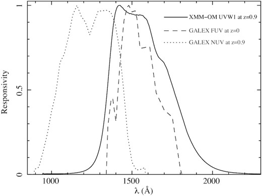
The rest-frame responsivity of the XMM-OM UVW1 passband at z = 0.9 compared to that of the GALEX FUV passband at z = 0 and the GALEX NUV passband at z = 0.9.
As part of this paper, we describe the optical and infrared imaging of the 13H Field and the techniques that were used to derive photometric redshifts. This material serves also as a reference for the data and techniques used in earlier works on the 13H Field that make use of these photometric redshifts (Seymour et al. 2009, 2010; Symeonidis et al. 2009).
This paper is laid out as follows. In Section 2, we describe the UV XMM-OM imaging that forms the basis of this study, and the supporting optical and infrared data that were used to derive redshifts. The methods used to construct the luminosity function are described in Section 3. Our results are presented in Section 4. Section 5 contains our discussion, and our conclusions are presented in Section 6. Appendix A describes some analysis of the supporting optical and infrared image properties that was required for the photometric redshift determination.
Throughout this paper, magnitudes are given in the AB system (Oke & Gunn 1983). We have assumed cosmological parameters H0 = 70 km s−1 Mpc−1, ΩΛ = 0.7, and Ωm = 0.3. Unless stated otherwise, uncertainties are given at 1σ.
2 OBSERVATIONS AND DATA REDUCTION
Our UV luminosity functions are based on a catalogue of sources detected in an XMM-OM UVW1 image, together with spectroscopic and photometric redshifts for the sources. Therefore, the UVW1 imaging, which has an effective wavelength of 2910 Å, is supported by optical spectroscopic observations and a coherent suite of optical, near-infrared, and mid-infrared imaging, from which high-quality photometric redshifts can be derived. The observations are described below; a summary of the imaging is given in Table 2.
2.1 XMM-OM UV imaging
The 13H field was observed with XMM–Newton over the course of three orbits in 2001 June (Loaring et al. 2005). The XMM-OM UVW1 observations comprised four exposures in full-frame, low-resolution mode of duration 5 ks each, for a total exposure of 20 ks.
Initial reduction of the XMM-OM data was carried out using the standard XMM–Newton Science Analysis Software (sas) version 12.0 task omichain, as far as the correction of each of the individual 5-ks exposures for modulo-8 noise via the sas task ommodmap. Then each exposure was corrected for background scattered light structure by subtracting a background template derived from many different XMM-OM fields observed through the UVW1 filter, and replacing it with a uniform background level at the mean of the subtracted template. The images were then corrected for distortion and aligned with the equatorial coordinate frame using the sas task omatt. The images were registered to the Sloan Digital Sky Survey (SDSS) astrometric reference frame by cross-correlating source positions derived from the XMM-OM images to the corresponding positions in the SDSS Data Release 6 (Adelman-McCarthy et al. 2008); the rms scatter between rectified XMM-OM and SDSS positions is 0.5 arcsec. Then, the images were co-added using the sas task ommosaic. The resulting image is shown in Fig. 2, and covers a sky area of 280.1 arcmin2.
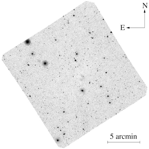
Co-added 20-ks XMM-OM UVW1 image of the 13H field.
Source detection and photometry were carried out with the sas task omdetect. This task uses a sequence of peak-finding and thresholding to find both point-like and extended sources. For point-like sources, photometry is measured in an aperture of 5.7-arcsec radius for bright sources, or 2.8-arcsec radius for faint sources, although intermediate aperture sizes are sometimes employed for measuring close pairs of objects. For extended sources the photometric aperture consists of all clustered pixels >2σ above the background level. For more details of the source detection procedure, see Page et al. (2012). A total of 734 sources were detected in the UVW1 image at a signal-to-noise threshold of 3, with the faintest objects detected having UVW1 magnitudes of 24.3.
2.2 Supporting optical spectroscopic observations
Optical spectroscopic observations provide precise redshifts. The 13H field has been used for extragalactic survey work for almost three decades, and so has a long history of spectroscopic observations targeting populations of sources selected at a variety of wavebands. Table 1 provides basic information on the spectroscopic campaigns that have furnished the majority of the redshifts used in this study. Principally, the redshifts come from observations with the William Herschel Telescope on La Palma, using the Autofib2 fibre-positioner together with the WYFFOS fibre-fed spectrograph, with Gemini GMOS and Keck LRIS and DEIMOS observations extending the follow-up to the faintest optical magnitudes.
Summary of optical spectroscopic observations.
| Observatory | Instrument | Wavelength | Resolution | Dates | Notes |
|---|---|---|---|---|---|
| range (Å) | (Å) | ||||
| WHT | AF2/WYFFOS | 3800–9200 | 20 | 1998/04/30–1998/05/04 | R300B grating, large fibres |
| Keck I | LRIS | 3800–9250 | 6.9 | 2002/04/12–2002/04/14 | 400/8500 red grating + 600/4000 blue grism |
| WHT | AF2/WYFFOS | 3800–9200 | 8.8 | 2002/05/09–2002/05/10 | R300B grating, small fibres |
| Keck II | DEIMOS | 4000–9500 | 3.5 | 2003/03/30–2003/03/31 | 600ZD grating |
| WHT | AF2/WYFFOS | 3800–9200 | 8.1 | 2003/03/30–2003/04/01 | R316R grating, small fibres |
| WHT | AF2/WYFFOS | 3800–9200 | 8.8 | 2006/04/25–2006/04/26 | R300B grating, small fibres |
| Gemini-N | GMOS | 4050–9600 | 11.1 | 2007/01/12–2008/05/08 | R150 grating, nod and shuffle |
| WHT | AF2/WYFFOS | 3800–9200 | 8.8 | 2014/06/02–2014/06/03 | R300B grating, small fibres |
| WHT | AF2/WYFFOS | 4800–9200 | 8.1 | 2015/05/08–2015/05/10 | R316R grating, small fibres |
A total of 168 UVW1 sources in the 13H field have spectroscopic redshifts. Their UVW1 magnitude distribution is shown in Fig. 3.
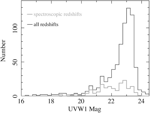
UVW1 magnitude distribution of extragalactic UVW1 sources. The bold grey histogram corresponds to the sources with spectroscopic redshifts, while the black histogram corresponds to sources with spectroscopic or photometric redshifts.
2.3 Supporting optical and infrared imaging
Here we describe the optical to infrared imaging observations that were used to derive photometric redshifts and to select targets for our optical spectroscopic observations. A total of 14 bands from u* to 8.0 μm are used here. The observational details are summarized in Table 2.
Summary of the optical, near-infrared, and mid-infrared imaging observations in the 13H field.
| Observatory | Instrument | Band | Dates | Ttot | Tused | Notes |
|---|---|---|---|---|---|---|
| XMM–Newton | XMM-OM | UVW1 | 2001/06/12–2001/06/24 | 20 000 | 20 000 | |
| Subaru | SuprimeCam | R | 2000/12/24–2000/12/25 | 5400 | 2400 | Central pointing, Chips w67c1,w93c2 faulty |
| R | 2003/05/02–2003/05/05 | 18 450 | 1 7550 | 3×3 mosaic | ||
| B | 2004/04/17–2004/12/16 | 10 800 | 7200 | Only 2004 Dec data useful | ||
| I | 2004/12/11 | 3000 | 3000 | |||
| z′ | 2004/04/17 | 4550 | 3150 | |||
| CFHT | MegaCam | u* | 2004/05/11–2005/04/06 | 20 786 | 20 786 | Single pointing |
| g′ | 2004/05/12–2005/07/10 | 21 606 | 21606 | |||
| i′ | 2004/05/09–2004/07/21 | 10 752 | 10 752 | |||
| INT | WFC | Z | 2006/03/03–2006/03/09 | 115 200 | 115 200 | 2×2 mosaic |
| CFHT | WIRCam | J | 2007/05/05–2007/07/08 | 17 360 | 17 360 | 2×2 mosaic |
| H | 2006/04/09–2007/07/13 | 31 110 | 31 110 | Two epochs of data | ||
| UKIRT | WFCAM | K | 2006/06/02–2006/06/06 | 45 480 | 45 480 | Filled tile |
| Spitzer | IRAC | All | 2005/06/15 | 36 525 | 36 525 |
Notes. Ttot is the total exposure time (in seconds) spent on sky, and Tused is the total exposure time of frames used in the the final stacks.
2.3.1 CFHT-Megacam u*, g′, and i′ data
We observed the 13H field using the CFHT-MEGACAM wide-field camera during 2004 and 2005. In total, 5.8, 6.2 and 3.0 h of useful exposure time were obtained in the u*, g′, and i′ bands, respectively. Fully calibrated stacked images and weight maps were downloaded from the MegaPipe (Gwyn 2008) website.1 The MegaPipe reduced images are photometrically and astrometrically tied to the SDSS imaging of the field.
2.3.2 Subaru SuprimeCam B, R, I, and z′ data
Observations of the 13H field were made using Subaru-SuprimeCam (Miyazaki et al. 2002). The first epoch of SuprimeCam imaging was carried out in the R band in 2000 December (McHardy et al. 2003), and further R-band imaging was obtained in 2003. B-, I-, and z′-band observations were obtained between 2004 April and December. For each epoch of imaging several jittered images were obtained per band to fill in the gaps between the individual CCD chips and to aid cosmic ray rejection.
Our reduction strategy drew heavily on the techniques described in detail by Erben et al. (2005) and Gawiser et al. (2006). We used a combination of standard iraf tools to debias, flat-field, and (for I and z′) remove the fringing. We then used TERAPIX (Bertin et al. 2002) and our own tools to calibrate the data astrometrically and photometrically, and to make the final stacked images.
2.3.3 INT-WFC Z-band data
We observed the 13H field in the Z band using the INT-WFC instrument over seven nights in 2006 March. The WFC data were detrended (debiased, flatfielded, superflattened) using standard iraf tools. Special attention was required to mitigate the effects of the strong and variable fringing (5–10 per cent of the sky level) seen in the Z band. The final image stack was made using scamp and swarp tools, combining a total of around 25 h of good data. The astrometry and photometry of the Z-band image were tied to the z′ measurements of stars and galaxies in the SDSS-DR6 catalogue.
2.3.4 CFHT-WIRCam J- and H-band data
We obtained observations of the 13H field in service mode with CFHT-WIRCam in the J and H bands during the 2006A and 2007A semesters. The data were preprocessed using CFHT’s iiwi WIRCam preprocessing pipeline. The TERAPIX team provided image stacks (Marmo 2007). The zero-points of the WIRCam images were tied to the 2MASS imaging in the 13H field.
2.3.5 UKIRT-WFCAM K-band data
We carried out imaging of the 13H field in the K band with UKIRT-WFCAM during 2006 June. A total of 21 h were obtained over five nights in good seeing conditions. Preprocessed and calibrated ‘interleaved’ stacks and weight images were obtained from the WSA archive.2 These images were combined to create a single stacked image and weight map using the scamp and swarp tools. The photometric calibration of the final stack was derived from the zero-points of the calibrated WSA data, which are derived from on-sky measurements of standard stars interspersed between the science observations.
2.3.6 Spitzer IRAC 3.6–8.0 μm data
An ∼30 × 60 arcmin2 stripe covering the 13H field was observed with Spitzer (Werner et al. 2004) during 2005 June and July. Data were obtained in all four IRAC bands (3.6, 4.5, 5.8, and 8.0 μm; Fazio et al. 2004). The exposure per pixel is approximately 500 s in each band. The IRAC basic calibrated data were processed using the standard Spitzermopex package (Makovoz & Khan 2005) to generate a mosaiced science image for each IRAC band. The standard Spitzer photometric calibration was adopted.
2.4 Determination of optical and infrared image characteristics
Several aspects of the images were characterized before we obtained the multiband photometry that was used to derive photometric redshifts. The PSF of each image was measured using bright, but not saturated, stars in the image, and aperture corrections derived. The limiting magnitude for each image, as a function of aperture size, was determined by analysis of the noise properties within randomly placed circular apertures. The bandpasses of the images were derived from the available information on the optical properties of the telescopes, instruments, and atmospheric extinction. Then, the zero-points were fine-tuned by fitting stellar templates to the spectral energy distributions of Galactic stars in the images. Each of these steps is described in more detail in Appendix A.
2.5 Multiband photometry method
We created a pipeline to make multiband photometric measurements of all objects detected in the optical and infrared imaging in the 13H field. First, a master catalogue of optical and infrared detections was created using SExtractor (Bertin & Arnouts 1996) to construct separate catalogues from the images in each filter. SExtractor was configured to record MAG_AUTO, MAGERR_AUTO, FLUX_RADIUS, and FLAGS parameters for each source (FLUX_RADIUS records the radius that contains 50 per cent of the source flux).
The individual SExtractor catalogues were then merged band by band into a master catalogue containing one row per unique source. The master catalogue is built up filter by filter and source by source. Detections across multiple bands are considered to be the same source if they lie within a small cross-matching radius (0.8 arcsec for the majority of the optical and NIR images, 1.0 arcsec for the J band, 1.2 arcsec for IRAC 3.6 and 4.5 μm, and 1.4 arcsec for IRAC 5.8 and 8 μm). The catalogue merging was ordered such that the deepest and most complete wavebands were added first, and the shallowest, least complete wavebands were added last. The position of any source detected across multiple bands was ‘refined’ by taking the signal-to-noise-weighted average of the individual positions of the source in each optical/NIR filter where it is significantly detected. These position refinements are typically small (<0.1 arcsec) but ensure that the position determined in any single band does not disproportionately affect the combined source position.
Aperture photometry in each band was then carried out at the location of each source in the master catalogue. The procedure utilized SExtractor in double image mode, where the ‘detection’ image is a synthetic image made with point sources placed at the locations of each master catalogue object. Aperture corrections were applied to account for the different PSFs in different passbands; see Appendix A for more details. In order to maximize the signal-to-noise ratio in the photometry of faint sources, and to reduce the aperture correction uncertainties for brighter, resolved galaxies, we have used different sized apertures depending on the apparent R magnitude of each source. For objects brighter than R = 18, we use a 5-arcsec diameter aperture, for objects with 18 < R < 20 a 3-arcsec aperture, and for fainter objects, we use a 2-arcsec diameter aperture.
2.6 Photometric redshift method
We have used the hyperz photometric redshift fitting package (Bolzonella, Miralles & Pelló 2000). We experimented with a number of sets of model galaxy SED templates, including the default template sets provided with hyperz (based on GISSEL98 synthesis models), the Coleman, Wu & Weedman (1980) set, and the Bruzual & Charlot (2003) templates. Of those we tried, we found that the galaxy template set presented in Rowan-Robinson et al. (2008) was best able to reproduce the spectroscopic redshifts of galaxies in the 13H field. The Rowan-Robinson et al. (2008) set consists of seven galaxy templates (E, E1, Sab, Sbc, Scd, Sdm, sb) plus three active galactic nucleus (AGN) templates. Extinction was modelled using the Calzetti et al. (2000) reddening law, with AV gridded in steps of 0.1 ranging up to 5.0 for the sb template, up to 2.0 for the Sdm template, up to 1.0 for the Sbc, Scd, and the three AGN templates, and no extinction allowed for the E, E1, and Sab galaxy templates. The absolute R-band magnitude was permitted to range over −27 < MR < −16.
For the purposes of running hyperz, we assumed zero Galactic redenning because the image zero-points have been calibrated against de-reddened stars that we assume lie behind the E(B − V) = 0.006 of Galactic dust (Schlegel, Finkbeiner & Davis 1998)3 seen in the direction of the 13H field. The magnitude uncertainties were increased by 0.05 mag in the IRAC bands to account for the zero-point and aperture correction uncertainties of the IRAC data. A minimum magnitude error threshold of 0.01 was adopted for all measurements in all filters. Our treatment for photometric measurements fainter than the nominal 1σ magnitude limit was to replace the measured flux with zero, and set the flux error to the 1σ value for the band in question.
The SEDs of AGN and starbursts at rest-frame wavelengths longer than 5 μm may become complicated by PAH and silicate features, as well as continuum emission from hot dust heated by an AGN. Therefore we have excluded IRAC 5.8- and 8.0-μm data from the photometric redshift fits for most objects. However, for faint, high-redshift (z ≫ 1) galaxies, the longer wavelength IRAC bands become useful as they can constrain the position of the redshifted 1.6-μm stellar bump. Therefore we include IRAC 5.8- and 8.0-μm data in the photometric redshift fit only for optically faint galaxies (R > 24) that have useful detections (magnitude error in 5.8- or 8.0-μm bands <0.3) and have flat or decreasing SEDs in the IRAC bands. Specifically, we require that [5.8] + 0.3 > [4.5] OR [8.0] + 0.3 > [5.8].
2.7 Photometric redshift fidelity
A comparison of our photometric redshifts to the redshifts of spectroscopically identified galaxies in the 13H field is shown in Fig. 4. Broad-line AGN (quasi-stellar objects, QSOs, and Seyfert 1 galaxies) are not shown, because continuum variability compromises photometric redshifts for such objects in studies such as ours, when the imaging in the different bands is not contemporaneous. For the 146 UVW1-detected galaxies that have spectroscopic redshifts, the photometric redshift residuals (δz = [zphoto − zspec]/[1 + zspec], where zphoto is the photometric redshift and zspec is the spectroscopic redshift) have an rms σδz = 0.042 and a mean, |$\overline{\delta z} = -0.005\pm 0.003$|. This scatter is comparable to the photo-z accuracy achieved in other deep photometric redshift studies (e.g. Babbedge et al. 2004; Ilbert et al. 2006; Mobasher et al. 2007; Rowan-Robinson et al. 2008). Adopting the definition from Ilbert et al. (2006) for a catastrophic failure of the photometric redshift as |δz| > 0.15, we find only one catastrophic failure out of the 146 UVW1-detected galaxies with spectroscopic redshifts.
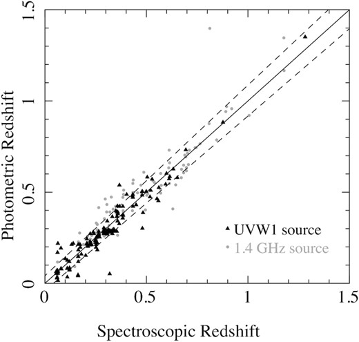
Photometric redshift against spectroscopic redshift for galaxies in the 13H field that have spectroscopic redshifts. In total,146 UVW1-selected galaxies (from this work) are shown as black triangles, and 174 1.4-GHz radio-selected galaxies (Seymour et al. 2008) are shown as grey dots. The solid line shows the one-to-one relation (solid) and the dashed lines indicate δz = ±0.042 (see Section 2.7).
The distribution of UVW1 magnitudes for sources with spectroscopic redshifts can be compared to the overall magnitude distribution of extragalactic sources in Fig. 3. While the spectroscopic sources span almost the full range of UVW1 magnitudes, the median UVW1 magnitude for galaxies (excluding broad-line AGN) with spectroscopic redshifts is 22.2, compared to 23.0 for galaxies with only photometric redshifts. Given this difference in the median magnitudes, we have derived the rms σδz separately for three UVW1 magnitude intervals to see how the scatter in photometric redshift changes with magnitude. For the magnitude intervals 21 < UVW1 ≤ 22, 22 < UVW1 ≤ 23, and UVW1 > 23, we obtain σδz of 0.046, 0.042, and 0.045, respectively. It appears that the accuracy of the photometric redshifts changes little with UVW1 magnitude to the limit of our UVW1-selected sample.
2.8 Association of UVW1 sources with optical counterparts
To match the UVW1 sources to counterparts in the optical, we have used our deep imaging in Johnson B taken with the SuprimeCam on the Subaru Telescope (see Section 2.3.2). UVW1 sources were matched to the brightest B-band source within 2 arcsec. This matching radius is similar to the PSF of the UVW1 images, and to the |$3\, \sigma$| positional error of XMM-OM sources once systematics related to the distortion correction are taken into account, and so represents a good compromise between maximizing the completeness of the associations and minimizing the number of incorrect associations. The median offset between UVW1 positions and those of their optical counterparts is 0.43 arcsec, and 95 per cent of the offsets are smaller than 1.25 arcsec.
2.9 Assignment of redshifts
UVW1 sources were attributed with the redshifts of the optical counterparts assigned in Section 2.8. Where available, spectroscopic redshifts were used in preference to photometric redshifts.
The list of UVW1-selected galaxies used for the construction of luminosity functions, together with photometry and redshifts, is given in Table 3.
UVW1-selected galaxies used to construct the luminosity functions.
| RA | Dec. | UVW1 mag | z | spec/phot |
|---|---|---|---|---|
| (J2000) | ||||
| 13 33 47.81 | + 37 53 08.7 | 23.169 ± 0.226 | 0.986 | phot |
| 13 33 50.09 | + 37 52 39.2 | 24.326 ± 0.358 | 0.738 | phot |
| 13 33 53.42 | + 37 54 40.7 | 22.945 ± 0.159 | 0.602 | phot |
| 13 33 53.87 | + 37 53 18.9 | 22.882 ± 0.178 | 0.855 | phot |
| 13 33 55.23 | + 37 52 49.0 | 23.227 ± 0.204 | 1.084 | phot |
Notes. The positions given are those derived from the UVW1 image. UVW1 mag is the UVW1 apparent magnitude in the AB system. The column labelled z gives the redshift for the source, and the column labelled spec/phot indicates whether the redshift is derived from spectroscopic or photometric data. Note that only the first five lines are included in the paper; the full table is available as supplementary material.
2.10 Exclusion of broad-line AGN
QSOs and Seyfert 1 galaxies are AGN characterized by broad emission lines and bright UV continua. Their UV radiation is powered by accretion on to their central supermassive black holes rather than originating in stars or stellar processes. The motivation to construct UV galaxy luminosity functions is to characterize the properties of star-forming galaxies, rather than AGN, and hence it is important to exclude these broad-emission-line AGN from the luminosity functions. In particular, because AGN can reach much higher UV luminosities than the stellar emission from galaxies, their inclusion would significantly distort the shape of the luminosity function at the brightest absolute magnitudes. Hence we exclude all objects spectroscopically identified as AGN with broad (FWHM >1000 km s−1) emission lines from the source list used to construct luminosity functions.
Fortunately, we are able to exclude these broad-line AGN quite thoroughly in the 13H XMM–Newton Deep Field. Their broad emission lines render them easier to identify and obtain redshifts through optical spectroscopy than other galaxies of comparable optical magnitudes, particularly at redshifts larger than 0.8. The original purpose of the 13H field was an X-ray and radio survey, primarily to study AGN emitting in these bands. As a result, AGN candidates have been the highest priority targets over many years of our spectroscopic follow-up campaigns. Five broad-line AGN with spectroscopic redshifts between 0.6 and 1.2 were excluded from our sample through this process.
As a further check for AGN contamination of the sample, we searched for UVW1 sources that are not spectroscopically identified, but which are within 2 arcsec of an X-ray source detected in our Chandra imaging observations (McHardy et al. 2003). We find three such sources. Their photometric redshifts are between 1 and 1.2, and their implied 0.5–7 keV X-ray luminosities at these redshifts are larger than 1043 erg s−1, higher than any known star-forming galaxy and implying that all three are AGN. Their implied UV absolute magnitudes range from −20.4 to −21.4, at the bright end of the luminosity function where AGN contamination could have a significant impact on luminosity function shape. In all three sources, there is a significant possibility that the UV emission is dominated by an AGN, and hence we excluded them from the sample.
3 CONSTRUCTION OF THE LUMINOSITY FUNCTION
3.1 Completeness
The completeness of the UVW1 source detection process as a function of magnitude was assessed by repeatedly injecting fake sources into the UVW1 image, repeating the source detection process, and recording the fraction of the injected sources that are recovered. The fake sources were given Gaussian spatial profiles with FWHM equivalent to the XMM-OM PSF, i.e. point-like sources. At the magnitudes and redshifts of interest (z > 0.6, UVW1 magnitude >21), almost all sources appear point-like to the omdetect source-detection software, and the 2.8-arcsec minimum-radius aperture used in omdetect to measure photometry renders the precise shape of the input source on sub-PSF scales unimportant. The positions of the fake sources were randomized over the image, and a single fake source was injected for each source detection pass. A source was considered to have been successfully recovered if a source was detected within 2 arcsec of the input position. A thousand injection/recovery trials were performed at each input magnitude tested to build up a statistically robust measurement of the completeness.
The results are shown in Fig. 5. The catalogue is 99 per cent complete for UVW1 ≤ 21 mag, 85 per cent complete at UVW1 = 23 mag, and falls to below 7 per cent by UVW1 = 24 mag. At the faint limit of the trials, UVW1 = 28.5 mag, simulated sources contribute an inconsequential number of counts to the image. The residual level of simulated source recovery at this magnitude, 0.4 per cent, represents the level of source confusion; at these magnitudes, the recovered sources are unrelated to the input sources, which are too faint to be detected.
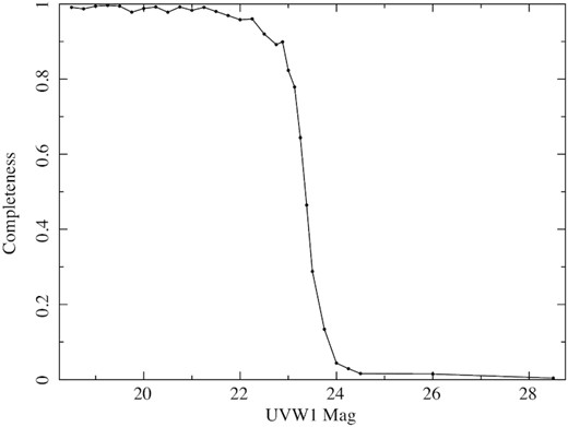
Completeness of the source detection as a function of UVW1 magnitude, as determined from the simulations described in Section 3.1.
3.2 Galactic extinction
The 13H field was chosen as an X-ray survey field because it has an exceptionally low Galactic H i column density of around 6 × 1019 cm−2 (Lockman, Jahoda & McCammon 1986; Branduardi-Raymont et al. 1994). It therefore has a correspondingly low level of Galactic extinction, which is beneficial for an extragalactic UV survey field. To determine the reddening correction we have used the extinction calibration from Schlafly & Finkbeiner (2011) together with the dust map of Schlegel et al. (1998). The inferred Galactic reddening in UVW1 in the direction of the 13H field is 0.027 mag, and all UVW1 magnitudes have been corrected for this level of Galactic reddening.
3.3 K-correction
K-correction, the correction of magnitudes from the observed wavelength passband to a fixed rest-frame passband is a critical step in the construction of luminosity functions, particularly in the UV where extinction leads to a large variation in spectral shape. For the reference rest-frame passband we have adopted the FUV channel of GALEX that has a peak response close to 1500 Å; this choice ensures that our results can be directly compared to the GALEX-derived UVLF of the local Universe (Wyder et al. 2005). Fortunately, the choice of the UVW1 passband for our XMM-OM observations (see Fig. 1), and its proximity to rest-frame 1500 Å for the redshift range of interest in our study (0.6 < z < 1.2), leads to a very modest range of K-correction. Fig. 6 shows K-corrections from the XMM-OM UVW1 passband (in the observer frame) to the GALEX FUV passband (in the rest frame) for the library of starburst templates presented by Kinney et al. (1996) and Calzetti et al. (1994). The template spectra have a short-wavelength limit of 1250 Å, and therefore cannot be used to derive K-corrections beyond z = 1. In order to facilitate K-correction to larger redshifts, we have extended the Kinney et al. (1996) SB 1 template to shorter wavelengths using the spectrum of the low-extinction starburst galaxy Mrk 66 from González et al. (1998). The K-corrections are almost template-independent at z = 0.9, and span a 0.4-mag range at the low-redshift limit of our sample, z = 0.6.
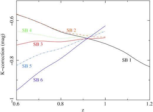
K-corrections for the starburst templates from Kinney et al. (1996) and Calzitti, Kinney & Storchi-Bergmann (1994), labelled as in Kinney et al. (1996). K-corrections for templates SB 2–6 end at z = 1 because the templates do not extend below 1250 Å. For template SB 1, the spectrum of Mrk 66 from González et al. (1998) has been used to extend the template to shorter wavelengths, permitting K-corrections to be derived to z = 1.2.
UV selection favours low-extinction galaxies, but to verify that the SB 1 template is appropriate for the K-correction we have compared the observed UVW1− u* colours of our galaxy sample with the synthesized colours of the template over the redshift range of interest. The results are shown in Fig. 7. The measurements are seen to be evenly distributed around the model curve throughout the redshift range of interest. Quantitatively, the mean UVW1 − u* colours for the observed galaxies are 〈UVW1 −u*〉 = 0.06 ± 0.04 for 0.6 < z < 0.8 and 〈UVW1 − u*〉 = 0.02 ± 0.05 for 0.8 < z < 1.2, in excellent agreement with the mean of the template curve, which is 0.07 in both redshift ranges.
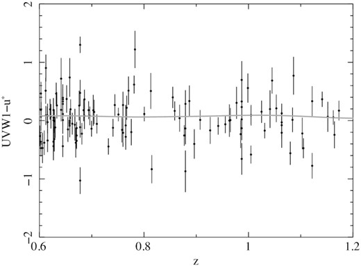
UVW1 −u* colours against redshift for the UVW1-selected galaxies in the 13H field (black data points) and the SB 1 galaxy template that is used for K-correction (grey curve).
3.4 Construction of the binned luminosity functions
The method of Page & Carrera (2000) was used to construct binned representations of the luminosity function. Two redshift ranges were chosen, 0.6 < z < 0.8 and 0.8 < z < 1.2 to allow direct comparison of our binned luminosity functions with those of Arnouts et al. (2005) and Hagen et al. (2015). For our survey, source completeness changes considerably between bright and faint magnitudes (Section 3.1 and Fig. 5). Completeness below unity is equivalent to a proportional reduction in survey volume. To take this effect into account, the effective sky area used to compute the binned luminosity functions was obtained by multiplying the sky area of the UVW1 image (280.1 arcmin2) by the source completeness in a series of discrete magnitude steps. The magnitude intervals and associated effective sky areas are given in Table 4. Uncertainties on the binned luminosity functions were computed according to Poisson statistics using the approach described in Gehrels (1986).
Effective sky area as a function of magnitude, used in the construction of the binned luminosity functions.
| UVW1 magnitude range | Effective sky area |
|---|---|
| (mag) | (arcmin2) |
| <18.50 | 279.0 |
| 18.50–21.75 | 276.8 |
| 21.75–22.25 | 274.3 |
| 22.25–22.50 | 271.8 |
| 22.50–22.75 | 260.3 |
| 22.75–23.00 | 243.0 |
| 23.00–23.25 | 185.0 |
| 23.25–23.50 | 89.3 |
| 23.50–23.75 | 43.2 |
| UVW1 magnitude range | Effective sky area |
|---|---|
| (mag) | (arcmin2) |
| <18.50 | 279.0 |
| 18.50–21.75 | 276.8 |
| 21.75–22.25 | 274.3 |
| 22.25–22.50 | 271.8 |
| 22.50–22.75 | 260.3 |
| 22.75–23.00 | 243.0 |
| 23.00–23.25 | 185.0 |
| 23.25–23.50 | 89.3 |
| 23.50–23.75 | 43.2 |
3.5 Measuring the Schechter function parameters
We used a parametric maximum-likelihood fit to the data to estimate the Schechter parameters α and M*. In the presence of photometric errors on the magnitudes, the observed luminosity function will be distorted from its original form in a manner analogous to the distortion of source counts by measurement errors (Eddington 1913). The following approach is analogous to the method developed by Murdoch, Crawford & Jauncey (1973) for radio source counts.
The probability distribution P(M′|M, z) is equivalent to the probability distribution of observed apparent UVW1 magnitudes m′ around the true apparent UVW1 magnitude m that corresponds to absolute magnitude M at redshift z. The distribution of observed versus true apparent magnitudes can be obtained directly from the simulations that were used to derive the completeness in Section 3.1. For our implementation of equation (5), we constructed histograms of m′ − m at a series of fixed values of m, spaced by 0.25 mag. The histograms were linearly interpolated to obtain a distribution appropriate for arbitrary m. The table of effective sky area for specific magnitude ranges (Table 4) was not employed for the maximum-likelihood fitting. Instead, completeness in the source detection is taken into account naturally in the fitting, because the histograms of m′ − m are normalized by the number of input sources in the simulations, but contain only those sources that were detected. This is equivalent to setting ∫P(M′|M, z)dM equal to the completeness at the apparent magnitude m corresponding to (M, z). Volume calculations assumed the full-sky area of the survey (280.1 arcmin2) to the limiting UVW1 magnitude of the survey (24.3 mag).
4 RESULTS
Our binned luminosity functions, constructed as described in Section 3.4, are shown in Fig. 8. The bins are 0.5 mag wide in absolute magnitude (M1500); the faintest bins are centred at M1500 = −18.95 and M1500 = −19.45 for the redshift ranges 0.6 < z < 0.8 and 0.8 < z < 1.2, respectively. In the 0.8 < z < 1.2 redshift range our binned luminosity function appears consistent with the Schechter function model obtained by Arnouts et al. (2005), but for 0.6 < z < 0.8 our binned luminosity function appears to be significantly steeper than the Arnouts et al. (2005) model. Tabulated values for the binned luminosity functions are provided in Table 5.
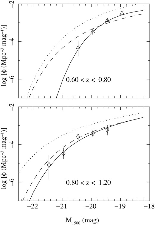
UV luminosity function of galaxies in the redshift intervals 0.6 < z < 0.8 (top panel) and 0.8 < z < 1.2 (bottom panel). The data points show the binned luminosity functions derived from the 13H field as described in Section 3.4, and the solid curves show the best-fitting Schechter functions derived according to the method described in Section 3.5. For comparison, the dashed lines show the best-fitting Schechter functions obtained by Arnouts et al. (2005), and the dotted lines show the maximum-likelihood Schechter functions obtained by Hagen et al. (2015).
Binned luminosity function measurements.
| Redshift range | M1500 | N | Log ϕ |
|---|---|---|---|
| (mag) | (log [Mpc−3 mag−1]) | ||
| 0.6 < z < 0.8 | −20.45 | 2 | |$-4.32^{+0.37}_{-0.45}$| |
| ″ | −19.95 | 13 | |$-3.48^{+0.13}_{-0.14}$| |
| ″ | −19.45 | 35 | −2.88 ± 0.08 |
| ″ | −18.95 | 25 | |$-2.49^{+0.09}_{-0.10}$| |
| 0.8 < z < 1.2 | −21.45 | 1 | |$-5.09^{+0.52}_{-0.76}$| |
| ″ | −20.95 | 4 | |$-4.47^{+0.25}_{-0.28}$| |
| ″ | −20.45 | 23 | −3.59 ± 0.10 |
| ″ | −19.95 | 15 | |$-3.42^{+0.12}_{-0.13}$| |
| ″ | −19.45 | 4 | |$-3.22^{+0.25}_{-0.28}$| |
Notes. M1500 is the centre of the absolute magnitude bin in the rest-frame GALEX FUV band; the absolute magnitude bins are 0.5 mag wide. N is the number of galaxies in the bin. ϕ is the luminosity function.
The results from our maximum-likelihood model fitting, as described in Section 3.5, are recorded in Table 6, and the confidence contours for α and M* are shown in Fig. 9. As is inevitable for a Schechter function fit to data that do not probe far into the faint, power-law section, the confidence contours are elongated, showing significant covariance between α and M*. According to the online tool4 provided by Trenti & Stiavelli (2008), cosmic variance contributes to the uncertainty on ϕ* at the level of 17 per cent in the redshift range 0.6 < z < 0.8, and 15 per cent for 0.8 < z < 1.2. The tool provided by Moster et al. (2011) gives slightly higher estimates, at 20 and 18 per cent, respectively.
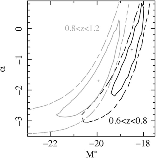
Confidence contours for the fitted Schechter parameters M* and α in the redshift intervals 0.6 < z < 0.8 (black) and 0.8 < z < 1.2 (grey). The solid and dashed contours correspond respectively to 68 and 95 per cent confidence for two interesting parameters.
Schechter function parameters from maximum-likelihood fitting.
| Redshift | N | α | M* | ϕ* | Mlim |
|---|---|---|---|---|---|
| interval | (mag) | (10−3 Mpc−3) | (mag) | ||
| 0.6–0.8 | 77 | −0.7 ± 1.1 | |$-18.5^{+0.4}_{-0.6}$| | |$10.5^{+2.2}_{-5.5}$| | −18.27 |
| 0.8–1.2 | 50 | |$-1.7^{+1.2}_{-0.8}$| | |$-19.9^{+0.6}_{-0.9}$| | |$1.2^{+0.9}_{-1.1}$| | −19.11 |
Notes. N is the number of galaxies included in the fit. Mlim gives the absolute magnitude in the rest-frame GALEX FUV band that corresponds to the limiting apparent magnitude in our survey (UVW1 = 24.3) at the central redshift of the relevant redshift interval.
5 DISCUSSION
We have constructed binned UV luminosity functions in the redshift ranges 0.6 < z < 0.8 and 0.8 < z < 1.2, and carried out maximum-likelihood fitting of Schechter function models to the unbinned data. To our knowledge, ours is the first study since Arnouts et al. (2005) to provide independent constraints on the UV luminosity function parameters in these two redshift ranges using a UV-selected sample of galaxies.
Our luminosity functions can be compared directly with the best-fitting models in the same redshift ranges derived by Arnouts et al. (2005) and Hagen et al. (2015) in Fig. 8. As Arnouts et al. (2005) and Hagen et al. (2015) carried out their studies in different regions of the sky to us, and to each other, differences in the normalization, and to a lesser extent M*, between the three studies are expected because of cosmic variance (Trenti & Stiavelli 2008; Moster et al. 2011). Ideally, cosmic variance would be overcome with the use of a statistical sample of independent UV survey fields, but at present there are only three. The study of Arnouts et al. (2005) is based on a larger area of sky than our study, or that of Hagen et al. (2015), and so we might expect it to probe the most representative range of large-scale structure environment. A simple estimate of the relative richness of our survey region compared to that of Arnouts et al. (2005) can be obtained by comparing the models around the faint limit of our survey, where we measure the largest space density of galaxies. In the redshift range 0.6 < z < 0.8, at M1500 = −19, our model for log ϕ is higher than that of Arnouts et al. (2005) by 0.2. If we were to assume that this difference represents an overdensity in the 13H field due to cosmic variance, comparison with fig. 7 of Trenti & Stiavelli (2008) suggests that we might expect our measurement of M* to be biased toward brighter absolute magnitudes by about 0.2 mag. We consider a potential bias of this size to be benign, because it is only half as large as the 1σ statistical uncertainty on M*. In the redshift range 0.8 < z < 1.2, at M1500 = −19.5, our model for log ϕ differs from that of Arnouts et al. (2005) by only 0.05, so we have no reason to expect any significant bias in our determination of M*.
The best-fitting α and M* parameters from our maximum-likelihood fitting, as well as those from other UV surveys covering similar redshift ranges, are shown in Fig. 10. The figure includes results from the studies of Cucciati et al. (2012) and Moutard et al. (2020), which we would describe as indirect measurements in the sense that they are based on surveys carried out at longer wavelengths from which UV luminosity functions are obtained by extrapolation to shorter wavelengths, albeit through sophisticated methods. These two works utilize large samples of galaxies compared to the direct studies, and so their results have relatively small statistical uncertainties. However, their measurements of α and M* show a similar degree of discrepancy with respect to each other as the measurements from the direct studies; consequently, in statistical terms, they are highly discrepant with each other. It would seem likely that systematics outweigh statistics as the dominant source of uncertainty in these indirect measurements, demonstrating the value of direct UV surveys to provide the ground truth in this redshift range.
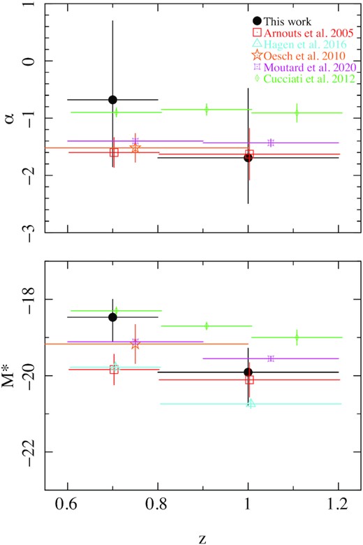
Measurements of Schechter function parameters α and M* from this work (closed black circles) and other UV surveys (open symbols). Data points from other surveys have been slightly offset in redshift to improve clarity.
It is evident from Fig. 8 that our binned luminosity functions in the two redshift ranges are different, with the 0.6 < z < 0.8 luminosity function appearing steeper than that of the 0.8 < z < 1.2 redshift range. In the maximum-likelihood fitting, the confidence contours for the two redshift ranges cover different regions in α and M* parameter space (Fig. 9). In contrast, evolution between the two redshift ranges can not be deduced from the Arnouts et al. (2005) study, either from inspection of their binned luminosity functions, or from the parameters derived from their maximum-likelihood fitting.
Inspection of the Schechter function parameters reported in Table 6 and their corresponding uncertainties confirms the impression given by Figs 8 and 9 that the evolution corresponds to a dimming of M* between 0.8 < z < 1.2 and 0.6 < z < 0.8; evolution in α is not suggested by the fits. With no prior assumption about α, the evolution in M* is significant at 2σ; if we were to assume that α = −1.5 in both redshift ranges, the significance of the change in M* would rise to 3σ.
Compared to the GALEX-based measurements in the same redshift range of Arnouts et al. (2005), our sample is smaller, covering a smaller sky area and with a shallower limiting magnitude. On the other hand, while the sample of Arnouts et al. (2005) suffers from systematics related to source confusion, this is a much smaller issue for our survey: the superior PSF of XMM-OM leads to minimal source confusion (<1 per cent).
A second issue in which we consider our XMM-OM survey to have an advantage over the GALEX study of Arnouts et al. (2005) is in the shape of the UVW1 bandpass compared to GALEX NUV for measuring rest-frame 1500-Å photometry at z > 0.6. In the construction of luminosity functions, the bandpass determines the K-correction, and so the suitability of the bandpass relates directly to the systematics associated with K-correction. A UVW1-based survey has the advantage that K-corrections for different spectral shapes converge at z = 0.9, and the range of K-corrections is small for the redshift range 0.6 < z < 1.2; see Fig. 6.
We can gauge the level of systematics inherent in our simple, single-template K-correction scheme by repeating our Schechter-function fit using a different template. This test is easily performed in the 0.6 < z < 0.8 range, for which we can derive K-corrections for any of our template spectra (see Fig. 6). We therefore repeated our Schechter-function fit, using the K-correction from the SB 6 template, the most different to the SB 1 template used to derive the results presented in Section 4. The best-fitting M* changes to −18.6, a difference of only 0.1 mag with respect to our original results, while the best-fitting faint-end slope changes to α = −1.5. These parameter changes are smaller than the corresponding 1σ statistical uncertainties for our study.
Arnouts et al. (2005) do not quantify the effect such systematics may have on their study; nor is it possible for us to quantify the effect of K-correction-related systematics on their study from the information that they provide. In qualitative terms, for GALEX NUV, the redshift at which K-corrections for different templates converge is z = 0.5, so the K-corrections for different spectral shapes will diverge progressively as redshift increases throughout the 0.6 < z < 1.2 range. Because GALEX NUV is a wide passband, Lyman α falls within its sensitive wavelength range throughout 0.6 < z < 1.2, and the wide variety of line profiles will induce additional scatter in the K-correction. Furthermore, the Lyman limit enters the GALEX NUV passband at z = 0.85, so K-corrections above this redshift depend on the escape fraction of Lyman continuum photons, about which little is known for galaxies in this redshift range, and which is likely to vary significantly between galaxies (Izotov et al. 2018). Hence K-corrections for the GALEX NUV band could be a non-trivial source of systematics in the construction of luminosity functions in this redshift range.
Our luminosity functions reach similar absolute magnitude limits to the luminosity functions constructed by Hagen et al. (2015) in the same redshift ranges, despite their Swift UVOT data having a much longer UVW1 exposure than our XMM-OM data. Hagen et al. (2015) based their study, which had somewhat broader goals than ours, on a master sample that was selected in the UVOT u filter and, as a result, the faint UV absolute magnitude limits were set by the onset of colour-dependent incompleteness. In their Schechter-function model fits, Hagen et al. (2015) fixed the faint-end slope α to the best-fitting values obtained by Arnouts et al. (2005); given the covariance between α and M*, their measurements of M* are therefore not strictly independent from those of Arnouts et al. (2005). None the less, their fits support the picture implied by our study that M* evolves such that it is brighter at 0.8 < z < 1.2 than at 0.6 < z < 0.8. Visual inspection of the binned luminosity functions of Hagen et al. (2015) also suggests that M* evolves in this fashion between the two redshift ranges.
In the redshift interval (0.5 < z < 1), that overlaps both of the redshift ranges that we have studied, Oesch et al. (2010) used the Hubble Space Telescope to measure the UV luminosity function to fainter magnitudes than Arnouts et al. (2005), Hagen et al. (2015), or us. Oesch et al. (2010) obtained α = −1.52 ± 0.25, which is consistent at 2σ with our measurements in both redshift ranges, and those of Arnouts et al. (2005).
One issue that deserves some attention is the potential contamination of UV galaxy luminosity functions by AGN. As discussed in Section 2.10, we have explicitly excluded from our luminosity functions QSOs and other AGN that we consider are likely to dominate the rest-frame UV emission of their hosts, using a combination of optical spectroscopy and X-ray indicators. Such AGN are small in number compared to star-forming galaxies: a total of eight AGN were excluded from our study, compared to more than 120 star-forming galaxies. However, several of these AGN have very bright absolute magnitudes, and, if included in the luminosity function, would contribute in absolute magnitude bins where star-forming galaxies are rare or absent from the sample. For our sample, inclusion of these AGN would make a material difference to the bright end of our 0.8 < z < 1.2 luminosity function. We find that with the AGN included, the best-fitting M* would brighten by more than a magnitude compared to that reported in Table 6. The best-fitting α would steepen to −2.5 and the shape of the confidence contours in the lower panel of Fig. 9 would change to imply much tighter constraints on α. Thus we find that the exclusion of UV-bright AGN is a critical step in constructing UV luminosity functions of galaxies.
With this finding in mind, it is interesting to note that the studies of Arnouts et al. (2005) and Hagen et al. (2015) make no mention of QSOs or AGN at all. Cucciati et al. (2012) do not explicitly say whether any kind of AGN are excluded from their luminosity functions. Moutard et al. (2020) do discuss QSOs as a contaminant in their luminosity functions, with the added complication that their photometric redshifts are probably wrong for QSOs. They do not describe the criteria by which they attempt to exclude UV-bright AGN. Oesch et al. (2010) exclude point-like sources in their Hubble imaging as a means of cleaning stars from their sample; at least powerful QSOs may be excluded by this method, but they do not discuss potential AGN contamination of their sample. In future we consider that it would be helpful for authors to outline explicitly the steps that they have taken to exclude UV-bright AGN from the samples of galaxies that they use to study the UV galaxy luminosity function, because this step has a significant impact on the luminosity functions that result.
Having carried out this study, which we hope will serve as a pilot for more extensive application of XMM-OM data to the measurement of galaxy UV luminosity functions, we make note of the following. Measurements of the faint-end slope α are rather poor between redshifts of 0.6 and 1.2 in all surveys. Averaging our measurement of α in the redshift range 0.8 < z < 1.2 with that of Arnouts et al. (2005), we still have a 1σ uncertainty of ±0.4, which is far from ideal. Further measurements of the faint-end slope are thus required if we are to determine the manner in which this parameter evolves as the Universe’s peak epoch of star formation came to a close. Given that the value of α is largely thought to be determined by feedback processes resulting from star formation (principally from supernovae and stellar winds), it could be argued that proper observational constraints on α are essential if we are to test models for the evolution of star formation with cosmic time. Better measurements of α demand luminosity functions that reach fainter absolute magnitude limits than the survey we have presented in this paper. Therefore progress here requires significantly deeper XMM-OM UVW1 observations than the 20-ks observation that formed the primary data in our study. Deeper observations already exist, which may be suitable for this purpose, though the collection and analysis of the required ancillary data sets for redshifts is a major task. Furthermore, so long as XMM–Newton continues operations there is potential for considerable improvements in UVW1 exposure time of deep extragalactic survey fields.
From the results of our study, it would appear that M* evolves significantly in the redshift interval 0.6 < z < 1.2, but the precision of our measurements should still be regarded as crude, particularly taking into account the covariance between M* and α. Better statistics at bright absolute magnitudes are essential for breaking down the statistical uncertainties on M*, and so larger sky area as well as deeper magnitude limits would be of benefit. Thanks to XMM–Newton’s long service, tens of square degrees of extragalactic sky have already been observed with XMM-OM in UVW1 (Page et al. 2012); hence, the XMM–Newton Science Archive could prove a rich resource for such a purpose if it can be combined with suitable redshift data.
6 CONCLUSIONS
We have used XMM-OM UVW1 imaging of the 13H extragalactic survey field to study the rest-frame 1500-Å luminosity function of galaxies in the redshift ranges 0.6 < z < 0.8 and 0.8 < z < 1.2. This is, to our knowledge, the first use of XMM-OM data to measure galaxy luminosity functions. The XMM-OM data are supported by a large body of optical and infrared imaging, as well as optical spectroscopy, to provide redshifts for the UV sources. Our binned luminosity functions are noticeably different for the two redshift ranges, indicating that the luminosity function evolved significantly during the corresponding period of cosmic history. We used maximum-likelihood fitting to fit Schechter-function models to the data. Our fits indicate that the characteristic break magnitude M* is brighter in the higher redshift interval. In contrast, evolution in this redshift range could not be inferred from the GALEX luminosity functions of Arnouts et al. (2005), though the Swift UVOT-based study of Hagen et al. (2015) did find some evidence that M* brightens with redshift in this redshift range. We argue that a combination of deeper, and wider area, XMM-OM UVW1 imaging could form an excellent basis for major improvement in our understanding of the UV galaxy luminosity function between redshifts of 0.6 and 1.2.
SUPPORTING INFORMATION
Table.txt
Please note: Oxford University Press is not responsible for the content or functionality of any supporting materials supplied by the authors. Any queries (other than missing material) should be directed to the corresponding author for the article.
ACKNOWLEDGEMENTS
This work was supported by Science and Technology Facility Council (STFC) grant numbers ST/N000811/1 and ST/S000216/1. DJW acknowledges support from an STFC Ernest Rutherford Fellowship. Based on observations obtained with XMM–Newton, an ESA science mission with instruments and contributions directly funded by ESA Member States and NASA. The WIRCam observations were made through the OPTICON program. This work is based in part on observations made with the Spitzer Space Telescope, which is operated by the Jet Propulsion Laboratory, California Institute of Technology under a contract with NASA. The William Herschel Telescope and the Isaac Newton Telescope are operated on the island of La Palma by the Isaac Newton Group of Telescopes in the Spanish Observatorio del Roque de los Muchachos of the Instituto de Astrofísica de Canarias.
DATA AVAILABILITY
The primary data underlying this paper are available from the XMM–Newton Science archive at https://www.cosmos.esa.int/web/xmm-newton (OBSIDs: 0109660801, 0109660901 and 0109661001). Supplementary data underlying this paper will be shared on reasonable request to the corresponding author.
Footnotes
Calculations were carried out assuming completeness of 50 per cent and a halo filling factor of 0.5.
REFERENCES
APPENDIX A: ANALYSIS OF OPTICAL AND INFRARED IMAGES
In order to reach the photometric precision required for reliable photometric redshifts, the PSFs, limiting magnitudes, and bandpasses of the optical and infrared images had to be measured. These characteristics were then used together with measurements of stars in the images to tweak the photometric zero-points. Each of these steps is described here. A summary of pertinent image characteristics is given in Table A1.
Summary characteristics of the UV, optical and infrared images of the 13H field.
| Band | λeff | Δλ | AB offset | A | IQ | |$\langle \Delta \underline{r} \rangle$| | ApCorr | 3σ depth | σZP | |
|---|---|---|---|---|---|---|---|---|---|---|
| (μm) | (μm) | (mag) | (deg2) | (arcsec) | (arcsec) | (mag) | (μJy) | (mag) | ||
| UVW1 | 0.291 | 0.079 | 1.362 | 0.078 | 2.61 | 0.43 | − | 24.3 | 0.69 | 0.05 |
| u* | 0.386 | 0.056 | 0.405 | 0.983 | 1.175 | 0.13 | 1.433 | 26.1 | 0.14 | 0.02 |
| B | 0.437 | 0.074 | −0.100 | 0.264 | 0.870 | 0.12 | 1.273 | 27.0 | 0.056 | 0.02 |
| g′ | 0.475 | 0.100 | −0.098 | 0.969 | 1.018 | 0.12 | 1.345 | 26.6 | 0.082 | 0.01 |
| R | 0.645 | 0.082 | 0.208 | 1.133 | 0.697 | 0.11 | 1.153 | 26.1 | 0.13 | 0.02 |
| i′ | 0.756 | 0.098 | 0.386 | 0.974 | 0.794 | 0.10 | 1.141 | 25.1 | 0.34 | 0.01 |
| I | 0.788 | 0.096 | 0.439 | 0.263 | 0.683 | 0.10 | 1.128 | 25.8 | 0.18 | 0.02 |
| z′ | 0.906 | 0.094 | 0.530 | 0.260 | 0.824 | 0.10 | 1.234 | 24.9 | 0.42 | 0.02 |
| Z | 0.906 | 0.103 | 0.534 | 1.063 | 1.302 | 0.13 | 1.778 | 23.7 | 1.2 | 0.05 |
| J | 1.248 | 0.109 | 0.942 | 0.464 | 0.686 | 0.12 | 1.159 | 23.3 | 1.7 | 0.03 |
| H | 1.616 | 0.200 | 1.372 | 0.473 | 0.670 | 0.14 | 1.187 | 22.9 | 2.5 | 0.03 |
| K | 2.190 | 0.247 | 1.900 | 0.791 | 0.806 | 0.15 | 1.172 | 23.0 | 2.3 | 0.03 |
| 3.6 μm | 3.513 | 0.505 | 2.818 | 0.434 | 2.25 | 0.20 | 1.359 | 23.0 | 2.3 | 0.10 |
| 4.5 μm | 4.443 | 0.670 | 3.290 | 0.439 | 2.00 | 0.21 | 1.397 | 22.6 | 3.4 | 0.10 |
| 5.8 μm | 5.647 | 0.950 | 3.783 | 0.433 | 2.32 | 0.28 | 1.650 | 20.6 | 23 | 0.10 |
| 8.0 μm | 7.617 | 1.950 | 4.424 | 0.435 | 2.85 | 0.28 | 1.841 | 20.5 | 23 | 0.10 |
Notes. λeff is the effective wavelength and Δλ is FWHM of the filter passband. AB offset gives the difference between Vega and AB magnitude systems for each band, in the sense AB mag = Vega mag + AB offset. A is the sky area covered with high-quality imaging (defined as the sky area where the weight map is at least 50 PER CENT of the median weight). IQ is the mean measured FWHM of point-like sources in the image. |$\langle \Delta \underline{r} \rangle$| is the median position difference between objects detected in the 13H field and objects in the SDSS-DR6 catalogue. ApCorr is the correction factor required to correct the flux measured in a 2-arcsec diameter aperture (3.8 arcsec for IRAC bands). The 3σ Depth columns give the faintest AB magnitude and flux density for a point source such that its total flux can be measured with a signal-to-noise ratio ≥3 using a 2-arcsec diameter aperture (3.8 arcsec for IRAC bands, 5.7 arcsec for UVW1). Note that for UVW1, these entries simply refer to the faintest magnitude detected in the image, while for the other bands, they were determined following the procedure described in Section A2. σZP is the estimated accuracy of the relative photometric calibration in this band.
A1 Image quality and aperture corrections
Our ground-based science images are each compiled by stacking a number of exposures, each obtained under different seeing conditions. The science images therefore have a complex PSF, which, in general, is unlikely to be well represented by a single Gaussian. However, a good knowledge of the PSF is necessary in order to calculate aperture corrections, and to discriminate between point-like and resolved objects. Therefore, in order to measure the PSF for each filter, we have produced a model PSF for each filter by stacking a large number of stellar objects detected in the science images. The following process was carried out for each optical/NIR band. First, a suitable subset of stellar objects were selected from the SDSS-DR6 catalogue. These stars were restricted to a magnitude range that is unsaturated in our imaging data. Small 150x150 pixel postage stamp images were cut out from around each star using swarp. Each postage stamp image was normalized to the total flux of the star (measured from the science image). These postage stamp images were reprojected on to a common pixel frame, and then, using swarp, were median averaged to produce a single PSF image per band. SExtractor is run on the resultant PSF postage stamp image to determine the image FWHM as well as the fractional flux enclosed as a function of aperture radius. This information is used to provide accurate aperture corrections for the photometric measurements used in this work. The FWHM of stellar sources in each band is listed in Table A1, as well as the multiplicative correction factor for a 2-arcsec diameter aperture. For the IRAC and MIPS bands, a good calibration is available on the IPAC website,5 and so the default FWHM and aperture correction factors were adopted.
A2 Image sensitivity and limiting magnitudes
In our final stacked images, the noise in adjacent pixels is somewhat correlated, due to the inevitable resampling step during the stacking process. Therefore, the raw rms of pixel values, scaled up to the aperture area, gives an underestimate of the true fluctuations due to sky noise. We have followed a similar technique to Gawiser et al. (2006) to calculate the rms noise fluctuations in each band. Essentially, SExtractor was used to measure the flux in a variety of different sized apertures at random positions on the science image. A histogram of the measured flux values was generated for each aperture sizes, and a Gaussian was fitted to the negative part of this histogram (the positive part contains contributions from astronomical objects). The widths of the Gaussians were then plotted against aperture area, to derive the sigma–area relation. The 3σ limiting magnitudes for a 2-arcsec aperture for each image band are listed in Table A1. Note that the faintest detectable source in each band will be somewhat fainter than these estimates because the detection process requires a significant enhancement over rather fewer pixels than covered by a 2-arcsec aperture.
A3 Determination of science filter bandpasses
In order to derive photometric redshifts we must know the effective transmission curves for each science filter. The effective bandpass of each filter is the product of not only the filter transmission, but also the detector quantum efficiency (QE), the reflectivity and transmission of the telescope plus instrument optics, as well as the atmospheric extinction. Each of these components can, in general, change the wavelength dependence of the effective transmission curve. For each science band we have downloaded the filter transmission and detector QE information from the website of the relevant observatory, as well as the reflectivity/transmission of the telescope and instrument optics where available. For each of the optical filters we have modified the transmission curve to approximate the effects of atmospheric extinction. To do this, we take the SDSS atmospheric transmission curve,6 suitable for 1 airmass at Apache Point Observatory (APO) and convert it into the appropriate average airmass during each set of science observations, taking into account the relative altitudes of the different observatories. For the NIR bands, we adopted the atmospheric extinction curve supplied by UKIRT, produced using the program IRTRANS4, and obtained from the UKIRT website.7
For each science filter between u* and H, we combined each of these components to generate an effective transmission curve. For the WFCAM K-band data, the effective transmission curve of Hewett et al. (2006) was adopted, which already incorporates all the necessary information.
For the IRAC data, the filter transmission curves for the 3.6-, 4.5-, 5.8-, and 8.0-μm bands were downloaded from the Spitzer website8 A plot of the transmission curves for the photometric filter set used in this paper is shown in Fig. A1. It can be seen that the entire range 0.3–8 μm is well sampled with the largest gap lying between the NIR and IRAC coverage.
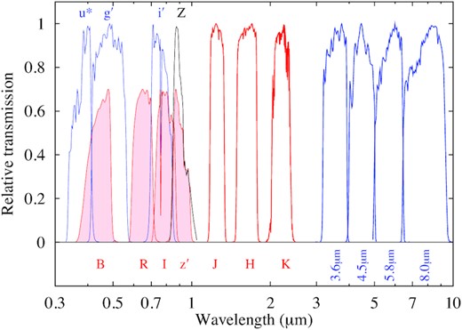
The effective system transmission curves for each band available for photometric redshifts in the 13H field. The transmission curves have been normalized to have a peak transmission of unity, except for the Subaru BRIz′ bands that, for clarity, are normalized to a peak of 0.7 (and shaded).
A4 Fine tuning of photometric zero-points
A crucial input for accurate and reliable photometric redshifts is to have accurately calibrated multiband photometry. Even small relative offsets in the zero-points of individual bands can significantly degrade the mean photometric accuracy and increase the rate of catastrophic redshift errors (classed here as |zphoto − zspec|/(1 + zspec) > 0.2). Therefore, to fine tune the relative zero-points of the optical/NIR imaging data we have devised a cross-calibration method using SDSS-DR6 and 2MASS photometric measurements of stellar objects within the 13H field. This method exploits the excellent photometric fidelity of the SDSS-DR6 and 2MASS surveys. In particular, we exploit the ‘Ubercalibrated’ magnitudes from the SDSS-DR6, which are absolutely calibrated to <0.02 mag (Ivezić et al. 2007).
Our procedure is to use the flux measurements of stars in the SDSS-DR6 ugriz and 2MASS JHKS bands to predict the magnitudes of these stars in the u*Bg′Ri′Iz′ZJHK science filter set (using a library of template and synthetic stellar spectra). These reference magnitudes are matched to the measured fluxes of these stars measured from the science images, and then it is then a simple task to find the best-fitting zero-point solution in each filter. This method guarantees that the science images themselves have been calibrated to a standard photometric system rather than deriving the calibration from e.g. a set of observations of standard stars that may have been observed at a range of airmasses and photometric conditions.
First, we select all stellar objects from the SDSS-DR6 catalogue that are covered by our science imaging of the 13H field. We apply the corrections (as suggested on the DR6 release notes9) to the SDSS magnitudes to bring them into the AB system: |$u^{\prime }_{\rm AB} = u^{\prime }_{\rm SDSS} -0.04$| and |$z^{\prime }_{\rm AB} = z^{\prime }_{\rm SDSS} +0.02$|. We use the ‘psfMags’ that are appropriate for stellar objects. We select the subset of stars that have no SDSS flags set, which have r′ < 22.5 and that have at least one filter measurement with an error less than 0.05 mag. We calculate the colours of each SDSS star relative to its ‘reference’ magnitude (defined as the mean of the magnitudes in the g′, r′, and i′ filters). We then choose a standard stellar spectral template that best matches the measured colours of each SDSS star, by folding the stellar template through the SDSS transmission curves. We initially adopted a set of stellar spectra from the Pickles (1998) and Bruzual–Persson–Gunn–Stryker (BPGS)10 stellar spectral libraries. However, we found that the locus in colour–colour space occupied by the SDSS stars in the 13H field was systematically offset (i.e. bluer in u′ − g′ for a given g′ − r′) from the colours of the BPGS/Pickles reference stars. This effect has been noted before in SDSS studies (e.g. Ivezić et al. 2007), where the measured location of the stellar locus in colour–colour space moves at a rate of ∼0.01 mag−1. In high Galactic latitude fields, at the faintest magnitudes (r′ ∼ 22) the reference stars are presumably located in the Galactic halo, and hence have lower than solar metallicity. To allow for this we supplemented our stellar template library with synthetic stellar templates from Castelli & Kurucz (2003), which span a wide range of metallicities, and which adequately span the colour–colour locus of the faint stars. The best-fitting stellar template is folded through the u*Bg′Ri′Iz′ZJHK filter bandpasses (see Section A3) to give the expected magnitudes of each SDSS reference star in each band.
Zero-points in each filter are then determined by a weighted least-squares fit to the measured image fluxes. This process results not only in a self-consistent calibration of magnitudes across all filters, but also good estimates of the residual calibration uncertainties.
We note that this process is similar to the method used to calibrate images in the MegaPipe pipeline, except that we calculate colour equations from stellar templates on a star by star basis rather than using empirical colour equations derived for a nominal stellar population (that may not be representative of the observed stars).
