


ABSTRACT
The knowledge of the ages of stars hosting exoplanets allows us to obtain an overview on the evolution of exoplanets and understand the mechanisms affecting their life. The measurement of the ages of stars in the Galaxy is usually affected by large uncertainties. An exception are the stellar clusters: For their coeval members, born from the same molecular cloud, ages can be measured with extreme accuracy. In this context, the project PATHOS is providing candidate exoplanets orbiting members of stellar clusters and associations through the analysis of high-precision light curves obtained with cutting-edge tools. In this work, we exploited the data collected during the second year of the Transiting Exoplanet Survey Satellite mission. We extracted, analysed, and modelled the light curves of |$\sim 90\, 000$| stars in open clusters located in the Northern ecliptic hemisphere in order to find candidate exoplanets. We measured the frequencies of candidate exoplanets in open clusters for different orbital periods and planetary radii, taking into account the detection efficiency of our pipeline and the false positive probabilities of our candidates. We analysed the age–RP distribution of candidate and confirmed exoplanets with periods <100 d and well constrained ages. While no peculiar trends are observed for Jupiter-size and (super-)Earth-size planets, we found that objects with |$4 \lesssim R_{\rm P} \lesssim 13R_{\rm Earth}$| are concentrated at ages ≲200 Myr; different scenarios (atmospheric losses, migration, etc.) are considered to explain the observed age–RP distribution.
1 INTRODUCTION
In Summer 2020, the Transiting Exoplanet Survey Satellite (TESS; Ricker et al. 2015) concluded its main mission after about 2 yr of observations. In this period, the spacecraft has observed millions of stars in about ≳70 per cent of the sky with an unprecedented photometric precision and temporal coverage, and new data from the extended mission, characterized by (in part) a new observing strategy, are coming.
Stellar clusters and associations offer the unique opportunity to derive precise stellar parameters (like radius, mass, chemical content, and especially age) for their members simply using theoretical models. During the main mission TESS observed many hundreds stellar (open and globular) clusters and associations in sectors of ∼27 d. However, the low resolution of the four cameras (∼21 arcsec pixel−1) makes the extraction of high-precision light curves difficult for the stars located in these dense regions.
The project ‘a PSF-based Approach to TESS High quality data Of Stellar clusters’ (PATHOS; Nardiello et al. 2019, hereafter Paper I) was born to exploit the TESS data in order to extract high-precision photometry for members of stellar clusters and associations adopting an innovative approach, based on the use of empirical point spread functions (PSFs) and neighbour subtraction. Scope of the project is the discovery and characterization of new candidate exoplanets in stellar clusters and the analysis of possible correlations between well-measured star properties and candidate exoplanet characteristics. Field stars’ age is usually affected by large uncertainties, but it is also an essential information to constrain the formation and understand the evolution of exoplanets, like for example how and on which temporal scales the mechanisms that bring to the atmosphere evaporation of low-mass close-in exoplanets happen (Lammer et al. 2003; Baraffe et al. 2005; Murray-Clay, Chiang & Murray 2009; Owen & Jackson 2012; Owen & Wu 2017; Wu 2019; Owen 2020). In this context, the PATHOS project is providing interesting candidate exoplanets orbiting stars with well constrained ages. Moreover, the high-precision light curves generated in our project, and publicly available to the astronomical community, allow us to obtain results not only in the research field of exoplanets, but also in other fields like asteroseismology (Mackereth et al. 2021), or the analysis of the spin axis orientations of cluster members (Healy & McCullough 2020).
We already successfully applied the PATHOS pipeline in Paper I, when we studied the stars in an extremely crowded region containing the globular cluster 47 Tuc and the Small Magellanic Cloud. In Nardiello et al. (2020, hereafter Paper II), we extracted and analysed the light curves of open cluster members located in the Southern ecliptic hemisphere, finding 33 objects of interest and deriving a first estimate of exoplanet frequency in open clusters. Nardiello (2020, hereafter Paper III) studied the light curves of the members of five young associations, having ages ≲10 Myr; in particular, the author performed a gyrochronological analysis of association members to constrain the age of the stars, analysed the dust in the circumstellar discs of the young members and identified and characterized six strong candidate exoplanets.
In this work, we exploited the TESS data collected during Cycle 2 (Sectors 14–26) to obtain high-precision light curves of cluster members in the Northern ecliptic hemisphere by using our cutting-edge tools (Section 2), find and characterize candidate exoplanets in stellar clusters (Section 3), and analyse their frequency and properties as a function of host stars’ characteristics (Sections 4). We summarized and discussed the joined results obtained in this work and in Paper II in Section 5.
2 OBSERVATION AND DATA REDUCTION
In this work, we extracted and analysed the light curves of the stars likely members of Northern ecliptic hemisphere open clusters observed by TESS during the second year of the mission. The observations used in this work were carried out between 2019 July 18 and 2020 July 4 (∼352 d), and are divided into 13 sectors (Sectors 14–26); in Sectors 21, 22, and 23, no open clusters fell in the TESS field of view and therefore the final number of analysed sectors is 10.
For the light-curve extraction and correction, we used the PATHOS pipeline described in detail in Papers I and II. We extracted the light curves of stars in a given catalogue from TESS full frame images (FFIs) by using the light-curve extractor IMG2LC. This software was developed by Nardiello et al. (2015a, 2016a) for ground-based observations, and it is a versatile tool that can be used with photometric time-series collected also with space-based observatories (see, e.g. Libralato et al. 2016a,b; Nardiello et al. 2016b).
The three main inputs of our PSF-based approach are (i) FFIs, (ii) PSFs, and (iii) input catalogue. For each star in the input catalogue, the light-curve extractor searches for the neighbours within a radius of 20 TESS pixels in the Gaia DR2 catalogue (Gaia Collaboration et al. 2018), transforms their positions and luminosities in the reference system of the FFI, models them by using a local PSF and then subtracts them from the FFI. Finally, it extracts PSF-fitting and aperture (1-, 2-, 3-, and 4-pixel radius) photometries of the target star from the neighbour-subtracted FFI. This approach has two advantages: (i) It minimizes the dilution effects due to the neighbour contaminants, and (ii) it allows us the extraction of high-precision photometry for stars in the TESS faint regime of magnitudes (T ≳ 15; see, e.g. Apai, Nardiello & Bedin 2021). We corrected the extracted raw light curves for systematic effects by fitting and applying the Cotrending Basis Vectors, as widely discussed in Papers I and II.
As in Paper II, we used as input list the catalogue of cluster members published by Cantat-Gaudin et al. (2018); this catalogue contains the positions, colours, magnitudes, proper motions, parallaxes, and membership probabilities of likely members in 1229 stellar clusters. From this catalogue, we selected all the stars that satisfy these two conditions: (i) magnitude G < 17.5, because stars with larger magnitude are too faint to be detected by TESS; and (ii) ecliptic latitude β > 4○, which corresponds to the part of the Northern ecliptic hemisphere covered by TESS.1
Fig. 1 shows the 126 372 stars (red points) in the input catalogue overlapped with the TESS fields of view (grey points): About 1/3 of them fall outside the TESS observations. We extracted 150 216 light curves of 89 858 stars in 411 clusters; about 50.3 per cent, i.e. 45 182 stars, were observed in only one sector, 30 957 stars (∼34.4 per cent) were observed in two sectors, 11 844 (∼13.2 per cent) in three sectors, and 1 875 (∼2.1 per cent) in four or more sectors.
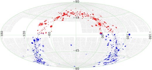
Aitoff projection in ecliptic coordinates of the fields observed by TESS in the first 2 yr of mission and of the open cluster members analysed in the PATHOS project: Grey points represent the sources observed in 2-min cadence mode in Sectors 1–26, and blue and red points are the stars in the input list used in Paper II and in this work, respectively.
Light curves are released on the Mikulski Archive for Space Telescopes (MAST) as a High Level Science Product (HLSP) under the project PATHOS2 (DOI: 10.17909/t9-es7m-vw14). A detailed description of the light curves (that are both in ascii and fits format) is reported in Papers I and II and in the MAST web page of the PATHOS project.
2.1 Photometric precision
We explored two different quality parameters, already defined in Papers I, II, and III, to identify for each star the photometric method that gives the best light curve.
The first quality parameter is the simple rms, defined as the 68.27th percentile of the 3.5σ-clipped sorted residual from the median value. This parameter is sensitive to the (high) variability of some stars, and, for this reason, is not recommended to estimate the photometric precision of the light curve. The mean trends of the rms as a function of the TESS magnitude T for the five photometric methods are reported in Fig. 2 (top panel).
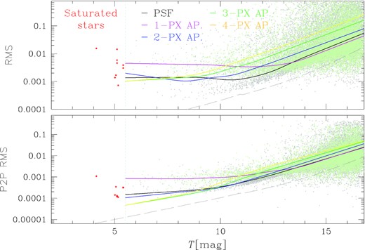
Mean trends of the photometric rms (top-panel) and P2P rms (bottom panel) as a function of the TESS magnitude T for different photometric methods: Black lines are associated with PSF-fitting photometry, and magenta, blue, green, and yellow lines are associated with 1-, 2-, 3-, and 4-pixel aperture photometries, respectively. As an example, the rms distributions obtained with 3-pixel and PSF-fitting photometry are shown in light green and grey crosses, respectively (for clarity, only 10 per cent of the stars are plotted). Red starred symbols represent the saturated stars. The dashed line is the theoretical limit calculated as in Paper II.
The second quality parameter is the P2P rms, defined as the 68.27th percentile of the 3.5σ-clipped sorted residual from the median value of the vector δFj = Fj − Fj + 1, with F the flux at a given epoch j. This parameter is not sensitive to the intrinsic luminosity variations of the stars, and we used it to define the interval in which each photometric method works, on average, better than the others. From the mean trends shown in bottom panel of Fig. 2, we found (confirming the results obtained in the previous works) that for stars with 5.5 ≲ T ≲ 7.0, the aperture photometry with radius 4-pixel gives the best results; the best photometric methods for the intervals 7.0 ≲ T ≲ 9.0, 9.0 ≲ T ≲ 10.0, and 10.0 ≲ T ≲ 13.0 are 3-pixel, 2-pixel aperture, and PSF-fitting photometries, respectively. For faint stars with T ≳ 13.0, the 1-pixel aperture photometry gives the lower P2P rms.
In the following analysis, we used, for each star of magnitude T⋆, the light curve associated with the photometric method that has the lower mean P2P rms in T⋆. We excluded from the analysis all the stars whose mean light-curve instrumental magnitude (Tinstr) is too different from the expected magnitude Tcalib, following this procedure: We extracted the δT = Tinstr − Tcalib distribution, we calculated its mean (|$\bar{\delta T}$|) and the standard deviation (σδT), and we excluded the ith light curve if |$|\delta T_i-\bar{\delta T}|\gt 4\sigma _{\delta T}$|. We also excluded all the light curves that have |$\lt 75\, {{\ \rm per\ cent}}$| of well-measured points (i.e. DQUALITY=0 and FLUX≠ 0). The final number of analysed light curves is 138 924 associated with 84 967 stars.
3 CANDIDATE EXOPLANETS: SEARCHING, VETTING, AND CHARACTERIZATION
We searched for signals of transiting objects among the selected light curves following the procedure described in Papers II and III. Briefly, we removed the intrinsic stellar variability interpolating the light curve with a fifth order spline defined on Nknots knots. In order to model short- and long-period variability, we considered two different grids of knots, with knots spaced by 6.5 and 13.0 h, respectively. The grids of knots are defined on continuous parts of light curves that does not present ‘breaks’ >0.5 d, in order to avoid the introduction of artifacts in the flattened light curve. We also removed from the light curves the photometric points associated with high values of the local sky (>5σSKY from the mean local background), with DQUALITY>0 and 4σ above the median normalized flux. We extracted the transit-fitting least-squares (TLS) periodograms of the flattened light curves adopting the Python package tls3 (Hippke & Heller 2019), and searched for transit signals with period 0.6 d ≤ P ≤ TLC, with TLC being the temporal length of the light curve. We used the output parameters for the first selection of candidate transiting objects, as follows: (i) We selected the stars associated with a depth of the transit |$\delta _{\rm t}\lt 10\, {{\ \rm per\ cent}}$| and to a significance between odd and even transits σodd-even < 2.5 ; (ii) we divided the signal detection efficiency (SDE) and the signal-to-noise ratio (SNR) distributions in bins of periods δP = 0.5 d, and calculated the 3.5σ-clipped mean and standard deviation of SDE (|$\bar{\rm SDE}$| and σSDE) and SNR (|$\bar{\rm SNR}$| and σSNR) within each bin. Then we interpolated the binned points |$\bar{\rm SDE} + 3.5\sigma _{\rm SDE}$| and |$\bar{\rm SNR} + 3.5\sigma _{\rm SNR}$| with a spline, and we selected as good candidates all the stars above these splines. Panels (a) of Fig. 3 show an example of selections based on the output parameters of TLS. We visually inspected the light curves that passed the above selections to exclude false positives due to the presence of artefacts. We applied the above procedure both to the light curves obtained in each single sector, and then to the stacked light curves of stars observed in more than one sector, in order to increase the efficiency of transit detection. The number of stars that passed the first-step selection is 279 (∼0.3 per cent).
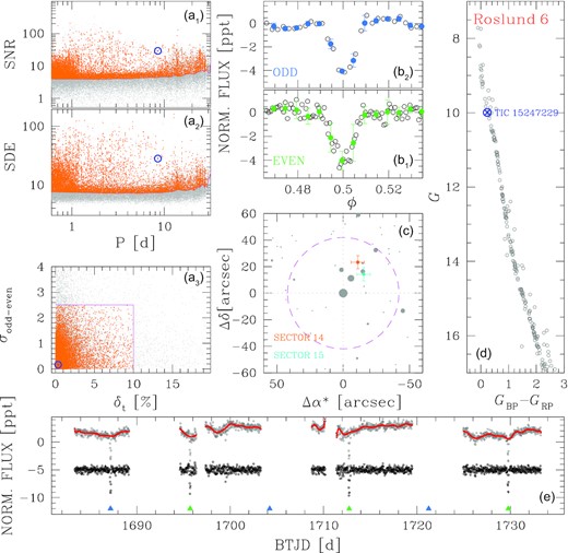
Candidate selection and vetting in the case of the star TIC 15247229 (TOI-1188). Panels (a1) and (a2) show the TLS SNR and SDE versus detected period, respectively, while panel (a3) reports the σodd-even as a function of δt; grey points are all the analysed stars, orange points the light curves that passed the selection described in the text, and the blue circle is TOI-1188. In panels (b1) and (b2), we compare the binned odd (azure) and even (green) transits of the candidate. Panel (c) represents the analysis of the in-/out-of-transit difference centroid: The centroid is shifted on a neighbour star that contaminates the target. Panel (d) is the G versus (GBP − GRP) colour–magnitude diagram (CMD) of Roslund 6, the open cluster that hosts TOI-1188 (blue circle). Panel (e) explains the procedure of flattening of the light curve: Grey points form the original, cleaned light curve; red line is the model defined by a spline on knots spaced by 13.0 h; and black points are the flattened light curve. Azure and green triangles indicate the odd and even transits, respectively.
These candidates were subjected to a series of vetting tests widely described in the previous papers of the PATHOS series. They are as follows: (i) Check for the transit depths in the light curves obtained with different photometric methods; (ii) check for the presence of secondary eclipses in the light curves phased with a period 0.5 × P, 1.0 × P, and 2.0 × P, with P the period found by the TLS routine; (iii) check for the transit depths by comparing binned odd/even transits (panels b of Fig. 3); and (iv) check for contamination through the analysis of the in/out-of-transit difference centroid (panel c of Fig. 3). After this second-step selection, 39 transiting objects of interest survived (∼0.05 per cent); one of these objects showed only one transit in its light curve.
3.1 TESS Objects of Interest
We cross-matched the TESS Objects of Interest (TOI) list4 with our input catalogue of cluster members. Four candidates, found by the Quick-Look Pipeline (QLP; Huang et al. 2020), are also in our input catalogue, but only one of them (TOI-1535, TIC 420288086) is in our final list of transiting objects of interest. Two of them (TOI-1497, TIC 371673488 and TOI-1321, TIC 195199644) were not detected by our pipeline because no transit signals are present in the light curves we analysed, even if the mean scatter of our light curves is lower than the scatter of the light curves shown in the QLP data validation report. We checked the notes about these two candidates on ExoFOP5: (i) the depth-aperture correlation for TOI-1497.01, reported in a note on ExoFOP, is confirmed by our analysis; (ii) for TOI-1321, a depth-aperture correlation is also reported; moreover, a note associated with a photometric follow-up with MuSCAT2 reports a deep transit signal from a nearby star at ∼1 arcmin from TOI-1321. Therefore, both these candidates are likely contaminated by neighbour sources. The fourth QLP candidate, TOI-1188 (TIC 15247229), was excluded from our final list after the centroid analysis. Its vetting tests are reported in Fig. 3. Our conclusion is also supported by the notes reported in the photometric follow-up section of the ExoFOP website.
3.2 Stellar parameters
We fitted theoretical models from the last release of BaSTI (‘a Bag of Stellar Tracks and Isochrones’) models (Hidalgo et al. 2018) to the CMDs of the 32 open clusters that host the stars associated with the 39 transiting objects of interest. In this way, we were able to extract primary information (stellar radius, mass, density, effective temperature) of the stars that host candidate transiting objects. Because metallicity measurements are not available for the large part of the clusters and because open clusters have, on average, metallicities similar to that of the Sun, in our fit, we used isochrones with [Fe/H] = 0.0 ± 0.3 as already done in Paper II, and we added the contribution of the uncertainties on the metallicity to the final errors on the stellar parameter estimates.
We transformed the isochrones from the theoretical to the observational plane using the distance modulus of the clusters obtained by Cantat-Gaudin et al. (2018), and the reddening and ages measured by Kharchenko et al. (2016), Röser et al. (2016), and Bossini et al. (2019); since some of the catalogues do not provides error estimates, for homogeneity, we used a conservative error of 10 per cent on the age and reddening values. Gulliver 49 is an open cluster discovered by Cantat-Gaudin et al. (2018), and no age estimate is provided in literature: We followed the technique by Nardiello et al. (2015b) based on the use of the χ2-minimization between isochrones and fiducial lines to derive an estimate of the cluster age. We found an age of 200 ± 20 Myr.
Clusters’ parameters adopted for the isochrone fitting are reported in Table 1. Stellar parameters of the transiting candidates’ hosts obtained from isochrone fitting were used as priors in transit modelling described in the next section, and are reported in Table A1.
Cluster parameters.
| Cluster name | Age | Distance | E(B − V) | Reference |
|---|---|---|---|---|
| (Myr) | (pc) | |||
| ASCC 13 | 44 ± 4 | 1078 ± 105 | 0.22 ± 0.02 | (1) |
| Alessi 37 | 133 ± 13 | 707 ± 46 | 0.25 ± 0.03 | (1) |
| Alessi Teutsch 5 | 74 ± 7 | 876 ± 70 | 0.50 ± 0.05 | (2) |
| Czernik 44 | 32 ± 3 | 4696 ± 1500 | 1.13 ± 0.11 | (2) |
| FSR 0342 | 376 ± 38 | 2687 ± 570 | 0.65 ± 0.07 | (2) |
| Gulliver 49 | 200 ± 20 | 1622 ± 425 | 1.15 ± 0.12 | (4) |
| IC 1396 | 1 ± 1 | 913 ± 76 | 0.42 ± 0.04 | (2) |
| King 5 | 1230 ± 123 | 2523 ± 510 | 0.67 ± 0.07 | (2) |
| King 6 | 382 ± 38 | 727 ± 50 | 0.59 ± 0.06 | (1) |
| King 20 | 349 ± 35 | 1093 ± 305 | 0.67 ± 0.07 | (1) |
| NGC 225 | 179 ± 18 | 684 ± 44 | 0.27 ± 0.03 | (1) |
| NGC 457 | 24 ± 2 | 2882 ± 650 | 0.60 ± 0.06 | (2) |
| NGC 752 | 1479 ± 148 | 441 ± 20 | 0.05 ± 0.01 | (1) |
| NGC 884 | 16 ± 2 | 2341 ± 445 | 0.56 ± 0.06 | (2) |
| NGC 1027 | 355 ± 35 | 1097 ± 98 | 0.45 ± 0.05 | (2) |
| NGC 6811 | 863 ± 86 | 1112 ± 101 | 0.07 ± 0.01 | (1) |
| NGC 6871 | 10 ± 1 | 1841 ± 285 | 0.60 ± 0.06 | (2) |
| NGC 6910 | 34 ± 3 | 1350 ± 260 | 1.20 ± 0.12 | (2) |
| NGC 6940 | 1023 ± 102 | 1025 ± 94 | 0.21 ± 0.02 | (1) |
| NGC 6997 | 552 ± 55 | 865 ± 70 | 0.53 ± 0.05 | (1) |
| NGC 7024 | 266 ± 27 | 1182 ± 130 | 0.63 ± 0.06 | (2) |
| NGC 7086 | 116 ± 12 | 1616 ± 225 | 0.77 ± 0.08 | (2) |
| NGC 7142 | 1778 ± 178 | 2376 ± 446 | 0.45 ± 0.05 | (2) |
| NGC 7209 | 341 ± 34 | 1178 ± 125 | 0.18 ± 0.02 | (1) |
| NGC 7245 | 355 ± 35 | 3307 ± 882 | 0.48 ± 0.05 | (2) |
| NGC 7510 | 50 ± 5 | 3177 ± 765 | 0.95 ± 0.09 | (2) |
| NGC 7654 | 79 ± 8 | 1600 ± 220 | 0.65 ± 0.07 | (2) |
| NGC 7789 | 1841 ± 184 | 2074 ± 366 | 0.22 ± 0.02 | (2) |
| RSG 5 | 50 ± 5 | 336 ± 11 | 0.04 ± 0.00 | (3) |
| RSG 8 | 316 ± 32 | 446 ± 20 | 0.04 ± 0.00 | (3) |
| SAI 25 | 243 ± 24 | 2194 ± 498 | 1.17 ± 0.12 | (2) |
| SAI 149 | 251 ± 25 | 3000 ± 690 | 1.24 ± 0.12 | (2) |
3.3 Transit modelling
We modelled the transits of the objects of interest using the python package pyorbit6(Malavolta et al. 2016, 2018, see also Benatti et al. 2019; Carleo et al. 2021; Lacedelli et al. 2021), based on the combined use of the package batman (Kreidberg 2015), the global optimization algorithm pyde7 (Storn & Price 1997), and the affine invariant Markov chain Monte Carlo sampler emcee (Foreman-Mackey et al. 2013).
For the transit modelling, we included the central time of the first transit (T0), the period (P), the impact parameter (b), the planetary-to-stellar-radius ratio (RP/R⋆), the stellar density (ρ⋆), and the dilution factor (df). The latter quantity is included as a free parameter, with a Gaussian prior obtained considering all the stars in the Gaia DR2 catalogue that fall in the same pixel of the target,8 and transforming their Gaia magnitudes in TESS magnitudes adopting the equations by Stassun et al. (2019). Host star parameters, like the stellar radius (R⋆), mass radius (M⋆), gravity (log g), and effective temperature (Teff) come from the isochrone fits described in the previous section. On the basis of log g and Teff, we obtained information on the limb-darkening (LD) by using the grid of values published by Claret (2018); we adopted the LD parametrization described by Kipping (2013). In the modelling process, the routine takes into account the local variability of the star by fitting a second-degree polynomial to the out-of-transit part of the light curve. The routine modelled the transits with a fixed circular orbital eccentricity (e = 0), and taking into account the 30-min cadence of the TESS FFIs (Kipping 2010).
The adopted priors on stellar parameters are reported in Table A1. The package pyorbit explored all the parameters in linear space. In the emcee run, the number of walkers used is 10 times the number of free parameters. We ran, for each model, the sampler for 80 000 steps, excluding the first 15 000 steps as burn-in and using a thinning factor of 100. Fig. 4 shows an example of the modelling process in the case of PATHOS-53, a mono-transit object of interest.
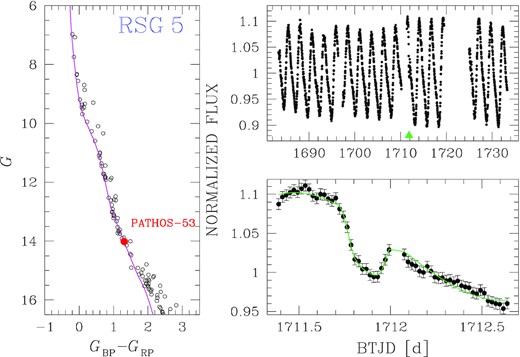
Overview on the transit modelling of PATHOS-53: The left-hand panel shows the G versus (GBP − GRP) CMD of the members of the open cluster RSG 5 and the isochrone fit (in magenta, tAGE = 50 Myr) used to derive the stellar parameters of PATHOS-53 (red point). The top right-hand panel shows the light curve of PATHOS-53 collected in Sectors 14 and 15; only one transit is detected (pointed by the green triangle). The bottom right-hand panel shows the model fit (green line) performed by pyorbit on the single transit.
In Table 2, we report the results of the transit fitting; Figs A1–A3 give an overview on the main properties of each transiting object of interest (position on the CMD, proper motions, in-/out-of-transit centroid analysis, transit modelling).
Results of transit modelling.
| TIC | PATHOS | Cluster | P | T0 | Rp/R⋆ | b | a | ρ⋆ | i | Rp | Rp | Note |
|---|---|---|---|---|---|---|---|---|---|---|---|---|
| (d) | (BTJD) | (au) | (ρ⊙) | (°) | (RJ) | (R⊕) | ||||||
| 0013416465 | 44 | NGC 6910 | |$5.5776_{ -0.0524}^{+ 0.0587}$| | |$1688.665_{-0.117}^{+0.105}$| | |$0.282_{-0.081}^{+0.144}$| | |$1.00_{ -0.13}^{+0.18}$| | |$0.0860_{-0.0005}^{+0.0006}$| | |$0.41_{ -0.01}^{+ 0.01}$| | |$84.2_{-1.1}^{+0.8}$| | |$5.16_{-1.49}^{+2.64}$| | |$57.79_{ -16.7}^{+ 29.6}$| | |
| 0013866376 | 45 | NGC 6910 | |$9.3972_{ -0.0031}^{+ 0.0032}$| | |$1686.476_{-0.005}^{+0.005}$| | |$0.075_{-0.006}^{+0.014}$| | |$0.93_{ -0.02}^{+0.03}$| | |$0.1575_{-0.0018}^{+0.0018}$| | |$0.12_{ -0.01}^{+ 0.01}$| | |$84.2_{-0.2}^{+0.2}$| | |$2.68_{-0.22}^{+0.52}$| | |$30.06_{ -2.5}^{+ 5.8}$| | |
| 0013875852 | 46 | NGC 6910 | |$8.3300_{ -0.0014}^{+ 0.0014}$| | |$1684.099_{-0.005}^{+0.005}$| | |$0.255_{-0.063}^{+0.166}$| | |$0.98_{ -0.10}^{+0.21}$| | |$0.1110_{-0.0003}^{+0.0003}$| | |$0.43_{ -0.01}^{+ 0.01}$| | |$85.7_{-0.9}^{+0.5}$| | |$4.54_{-1.13}^{+2.95}$| | |$50.91_{ -12.7}^{+ 33.1}$| | |
| 0050361536 | 47 | NGC 1027 | |$12.9725_{ -0.0086}^{+ 0.0088}$| | |$1793.465_{-0.006}^{+0.006}$| | |$0.327_{-0.100}^{+0.106}$| | |$1.22_{ -0.11}^{+0.11}$| | |$0.1482_{-0.0014}^{+0.0013}$| | |$0.15_{ -0.01}^{+ 0.01}$| | |$84.3_{-0.5}^{+0.5}$| | |$8.28_{-2.54}^{+2.68}$| | |$92.75_{ -28.4}^{+ 30.0}$| | |
| 0051022999 | 48 | NGC 1027 | |$7.7336_{ -0.0019}^{+ 0.0020}$| | |$1794.506_{-0.003}^{+0.003}$| | |$0.219_{-0.006}^{+0.006}$| | |$0.08_{ -0.05}^{+0.08}$| | |$0.0736_{-0.0003}^{+0.0003}$| | |$1.77_{ -0.01}^{+ 0.01}$| | |$89.8_{-0.2}^{+0.2}$| | |$1.69_{-0.04}^{+0.04}$| | |$18.99_{ -0.5}^{+ 0.5}$| | |
| 0065557265 | 49 | NGC 7789 | |$1.6828_{ -0.1092}^{+ 0.0002}$| | |$1785.339_{-0.063}^{+0.011}$| | |$0.114_{-0.094}^{+0.138}$| | |$0.75_{ -0.11}^{+0.22}$| | |$0.0318_{-0.0013}^{+0.0004}$| | |$0.55_{ -0.34}^{+ 0.32}$| | |$79.8_{-1.8}^{+2.7}$| | |$1.42_{-1.18}^{+3.29}$| | |$15.93_{ -13.2}^{+ 36.9}$| | |
| 0067424670 | 50 | NGC 752 | |$1.1328_{ -0.0001}^{+ 0.0001}$| | |$1790.941_{-0.001}^{+0.001}$| | |$0.188_{-0.006}^{+0.006}$| | |$0.71_{ -0.03}^{+0.03}$| | |$0.0200_{-0.0001}^{+0.0001}$| | |$1.92_{ -0.01}^{+ 0.01}$| | |$82.8_{-0.3}^{+0.4}$| | |$1.39_{-0.04}^{+0.05}$| | |$15.53_{ -0.5}^{+ 0.5}$| | |
| 0106235729 | 51 | NGC 6871 | |$4.0550_{ -0.0003}^{+ 0.0003}$| | |$1684.418_{-0.002}^{+0.002}$| | |$0.366_{-0.051}^{+0.060}$| | |$1.11_{ -0.06}^{+0.07}$| | |$0.0730_{-0.0003}^{+0.0003}$| | |$0.40_{ -0.01}^{+ 0.01}$| | |$81.9_{-0.5}^{+0.5}$| | |$7.08_{-0.99}^{+1.16}$| | |$79.41_{ -11.1}^{+ 13.0}$| | |
| 0154304816 | 52 | Alessi 37 | |$3.8552_{ -0.0009}^{+ 0.0009}$| | |$1742.164_{-0.002}^{+0.002}$| | |$0.259_{-0.119}^{+0.162}$| | |$1.12_{ -0.15}^{+0.17}$| | |$0.0537_{-0.0001}^{+0.0001}$| | |$0.57_{ -0.01}^{+ 0.01}$| | |$82.5_{-1.2}^{+1.0}$| | |$3.39_{-1.57}^{+2.12}$| | |$38.02_{ -17.6}^{+ 23.8}$| | |
| 0185779182 | 53 | RSG 5 | |$70.0427_{-19.5648}^{+ 19.4350}$| | |$1711.871_{-0.004}^{+0.004}$| | |$0.228_{-0.011}^{+0.012}$| | |$0.49_{ -0.25}^{+0.12}$| | |$0.3046_{-0.0598}^{+0.0541}$| | |$1.74_{ -0.17}^{+ 0.17}$| | |$89.7_{-0.1}^{+0.1}$| | |$1.69_{-0.10}^{+0.12}$| | |$18.99_{ -1.1}^{+ 1.3}$| | |
| 0251494772 | 54 | SAI 25 | |$5.3034_{ -0.0023}^{+ 0.0024}$| | |$1795.088_{-0.006}^{+0.005}$| | |$0.121_{-0.004}^{+0.004}$| | |$0.72_{ -0.04}^{+0.04}$| | |$0.0894_{-0.0014}^{+0.0014}$| | |$0.05_{ -0.01}^{+ 0.01}$| | |$81.4_{-0.9}^{+0.8}$| | |$4.70_{-0.29}^{+0.34}$| | |$52.64_{ -3.3}^{+ 3.8}$| | |
| 0251975224 | 55 | King 20 | |$3.5618_{ -0.0008}^{+ 0.0008}$| | |$1956.781_{-0.004}^{+0.003}$| | |$0.187_{-0.004}^{+0.004}$| | |$0.08_{ -0.06}^{+0.08}$| | |$0.0531_{-0.0001}^{+0.0001}$| | |$0.46_{ -0.01}^{+ 0.01}$| | |$89.4_{-0.6}^{+0.4}$| | |$2.73_{-0.06}^{+0.06}$| | |$30.65_{ -0.7}^{+ 0.7}$| | |
| 0260167199 | 56 | IC 1396 | |$17.6348_{ -0.0077}^{+ 0.0078}$| | |$1741.326_{-0.005}^{+0.005}$| | |$0.312_{-0.106}^{+0.120}$| | |$1.13_{ -0.13}^{+0.13}$| | |$0.1494_{-0.0004}^{+0.0004}$| | |$0.46_{ -0.01}^{+ 0.01}$| | |$87.1_{-0.3}^{+0.3}$| | |$4.44_{-1.51}^{+1.70}$| | |$49.72_{ -16.9}^{+ 19.0}$| | |
| 0269519402 | 57 | Gulliver 49 | |$3.3736_{ -0.0000}^{+ 0.0000}$| | |$1806.271_{-0.001}^{+0.001}$| | |$0.120_{-0.002}^{+0.002}$| | |$0.39_{ -0.07}^{+0.05}$| | |$0.0630_{-0.0005}^{+0.0005}$| | |$0.18_{ -0.01}^{+ 0.01}$| | |$85.9_{-0.7}^{+0.8}$| | |$2.95_{-0.09}^{+0.09}$| | |$33.07_{ -1.0}^{+ 1.0}$| | |
| 0270022396 | 58 | NGC 7654 | |$3.7786_{ -0.0000}^{+ 0.0000}$| | |$1807.429_{-0.001}^{+0.001}$| | |$0.347_{-0.056}^{+0.055}$| | |$1.12_{ -0.07}^{+0.07}$| | |$0.0666_{-0.0002}^{+0.0002}$| | |$0.36_{ -0.01}^{+ 0.01}$| | |$81.1_{-0.5}^{+0.6}$| | |$6.66_{-1.08}^{+1.05}$| | |$74.71_{ -12.1}^{+ 11.8}$| | |
| 0270618239 | 59 | NGC 6811 | |$2.6377_{ -0.0002}^{+ 0.0002}$| | |$1683.548_{-0.002}^{+0.002}$| | |$0.217_{-0.003}^{+0.003}$| | |$0.03_{ -0.02}^{+0.03}$| | |$0.0381_{-0.0001}^{+0.0001}$| | |$1.08_{ -0.01}^{+ 0.01}$| | |$89.8_{-0.2}^{+0.1}$| | |$2.10_{-0.03}^{+0.03}$| | |$23.56_{ -0.3}^{+ 0.4}$| | |
| 0270920839 | 60 | Czernik 44 | |$5.2236_{ -0.0001}^{+ 0.0001}$| | |$1768.090_{-0.002}^{+0.002}$| | |$0.151_{-0.010}^{+0.008}$| | |$0.81_{ -0.03}^{+0.02}$| | |$0.1088_{-0.0012}^{+0.0011}$| | |$0.12_{ -0.02}^{+ 0.02}$| | |$82.6_{-0.6}^{+0.6}$| | |$5.42_{-0.35}^{+0.39}$| | |$60.80_{ -3.9}^{+ 4.3}$| | |
| 0271443321 | 61 | SAI 149 | |$5.9718_{ -0.0001}^{+ 0.0001}$| | |$1765.415_{-0.002}^{+0.002}$| | |$0.393_{-0.026}^{+0.030}$| | |$0.89_{ -0.04}^{+0.05}$| | |$0.0970_{-0.0019}^{+0.0019}$| | |$0.07_{ -0.01}^{+ 0.01}$| | |$80.9_{-0.5}^{+0.4}$| | |$14.17_{-1.00}^{+1.15}$| | |$158.79_{ -11.2}^{+ 12.9}$| | |
| 0285249796 | 62 | ASCC 13 | |$4.7520_{ -0.0009}^{+ 0.0009}$| | |$1816.836_{-0.002}^{+0.002}$| | |$0.257_{-0.008}^{+0.008}$| | |$0.64_{ -0.04}^{+0.03}$| | |$0.0664_{-0.0001}^{+0.0001}$| | |$0.52_{ -0.01}^{+ 0.01}$| | |$86.2_{-0.2}^{+0.2}$| | |$3.72_{-0.12}^{+0.12}$| | |$41.70_{ -1.3}^{+ 1.4}$| | |
| 0298292983 | 63 | NGC 6940 | |$1.2816_{ -0.0131}^{+ 0.0001}$| | |$1701.051_{-0.052}^{+0.002}$| | |$0.146_{-0.016}^{+0.005}$| | |$0.76_{ -0.08}^{+0.05}$| | |$0.0267_{-0.0002}^{+0.0001}$| | |$0.33_{ -0.02}^{+ 0.02}$| | |$77.2_{-1.1}^{+1.5}$| | |$2.37_{-0.28}^{+0.14}$| | |$26.60_{ -3.2}^{+ 1.6}$| | |
| 0316246231 | 64 | King 6 | |$8.5751_{ -0.0020}^{+ 0.0020}$| | |$1795.982_{-0.002}^{+0.002}$| | |$0.360_{-0.065}^{+0.073}$| | |$1.12_{ -0.08}^{+0.09}$| | |$0.0992_{-0.0002}^{+0.0002}$| | |$0.43_{ -0.01}^{+ 0.01}$| | |$85.2_{-0.4}^{+0.4}$| | |$5.63_{-1.01}^{+1.14}$| | |$63.14_{ -11.3}^{+ 12.8}$| | |
| 0323717669 | 65 | RSG 8 | |$4.2378_{ -0.0015}^{+ 0.0018}$| | |$1955.852_{-0.007}^{+0.006}$| | |$0.169_{-0.008}^{+0.008}$| | |$0.14_{ -0.10}^{+0.14}$| | |$0.0453_{-0.0002}^{+0.0002}$| | |$2.66_{ -0.01}^{+ 0.01}$| | |$89.5_{-0.5}^{+0.4}$| | |$1.05_{-0.05}^{+0.05}$| | |$11.77_{ -0.6}^{+ 0.5}$| | |
| 0326483210 | 66 | FSR 0342 | |$3.8130_{ -0.0004}^{+ 0.0004}$| | |$1741.329_{-0.003}^{+0.003}$| | |$0.200_{-0.010}^{+0.007}$| | |$0.35_{ -0.10}^{+0.07}$| | |$0.0603_{-0.0005}^{+0.0005}$| | |$0.33_{ -0.01}^{+ 0.01}$| | |$87.2_{-0.6}^{+0.8}$| | |$3.55_{-0.17}^{+0.14}$| | |$39.80_{ -2.0}^{+ 1.6}$| | |
| 0332258412 | 67 | NGC 457 | |$7.1465_{ -0.0035}^{+ 0.0035}$| | |$1794.905_{-0.004}^{+0.004}$| | |$0.371_{-0.068}^{+0.074}$| | |$1.10_{ -0.09}^{+0.09}$| | |$0.1235_{-0.0005}^{+0.0005}$| | |$0.22_{ -0.01}^{+ 0.01}$| | |$83.3_{-0.5}^{+0.6}$| | |$10.19_{-1.88}^{+2.03}$| | |$114.24_{ -21.0}^{+ 22.8}$| | |
| 0334949878 | 68 | Alessi Teutsch 5 | |$19.4784_{ -0.0002}^{+ 0.0002}$| | |$1741.392_{-0.001}^{+0.001}$| | |$0.349_{-0.048}^{+0.055}$| | |$1.26_{ -0.05}^{+0.06}$| | |$0.2126_{-0.0011}^{+0.0010}$| | |$0.28_{ -0.01}^{+ 0.01}$| | |$86.4_{-0.2}^{+0.2}$| | |$7.76_{-1.06}^{+1.22}$| | |$87.01_{ -11.9}^{+ 13.7}$| | |
| 0348608380 | 69 | NGC 884 | |$16.3026_{ -0.2298}^{+ 0.5559}$| | |$1806.922_{-0.003}^{+0.003}$| | |$0.380_{-0.058}^{+0.064}$| | |$1.11_{ -0.07}^{+0.08}$| | |$0.2476_{-0.0024}^{+0.0056}$| | |$0.19_{ -0.02}^{+ 0.02}$| | |$85.9_{-0.3}^{+0.3}$| | |$12.60_{-1.93}^{+2.22}$| | |$141.26_{ -21.6}^{+ 24.9}$| | |
| 0356973763 | 70 | NGC 6997 | |$10.0250_{ -0.4778}^{+ 0.0035}$| | |$1720.499_{-0.328}^{+0.155}$| | |$0.104_{-0.017}^{+0.113}$| | |$0.92_{ -0.18}^{+0.09}$| | |$0.1182_{-0.0029}^{+0.0014}$| | |$0.13_{ -0.02}^{+ 0.02}$| | |$84.5_{-0.9}^{+1.1}$| | |$2.71_{-0.58}^{+2.94}$| | |$30.34_{ -6.5}^{+ 33.0}$| | |
| 0377619148 | 71 | NGC 7510 | |$19.8963_{ -0.1048}^{+ 0.0004}$| | |$1784.408_{-0.002}^{+0.002}$| | |$0.373_{-0.077}^{+0.077}$| | |$1.17_{ -0.09}^{+0.09}$| | |$0.2713_{-0.0065}^{+0.0062}$| | |$0.05_{ -0.01}^{+ 0.01}$| | |$84.1_{-0.4}^{+0.5}$| | |$18.65_{-3.85}^{+3.81}$| | |$209.06_{ -43.2}^{+ 42.7}$| | |
| 0408094816 | 72 | NGC 7142 | |$5.4037_{ -0.0001}^{+ 0.0001}$| | |$1743.980_{-0.002}^{+0.003}$| | |$0.172_{-0.005}^{+0.005}$| | |$0.52_{ -0.13}^{+0.08}$| | |$0.0711_{-0.0003}^{+0.0003}$| | |$0.09_{ -0.01}^{+ 0.02}$| | |$84.8_{-1.2}^{+1.5}$| | |$4.41_{-0.37}^{+0.38}$| | |$49.40_{ -4.2}^{+ 4.2}$| | |
| 0408358709 | 73 | NGC 7142 | |$6.3320_{ -0.0001}^{+ 0.0001}$| | |$1741.434_{-0.002}^{+0.002}$| | |$0.337_{-0.090}^{+0.108}$| | |$1.03_{ -0.13}^{+0.13}$| | |$0.0778_{-0.0003}^{+0.0003}$| | |$0.14_{ -0.01}^{+ 0.02}$| | |$82.1_{-1.0}^{+1.2}$| | |$7.40_{-2.12}^{+2.29}$| | |$82.92_{ -23.8}^{+ 25.7}$| | |
| 0417058223 | 74 | NGC 7086 | |$5.4767_{ -0.0005}^{+ 0.0004}$| | |$1712.263_{-0.002}^{+0.002}$| | |$0.347_{-0.078}^{+0.086}$| | |$1.18_{ -0.09}^{+0.10}$| | |$0.0853_{-0.0003}^{+0.0003}$| | |$0.31_{ -0.01}^{+ 0.01}$| | |$82.3_{-0.6}^{+0.6}$| | |$7.04_{-1.57}^{+1.74}$| | |$78.89_{ -17.6}^{+ 19.5}$| | |
| 0420288086 | 75 | NGC 225 | |$6.5343_{ -0.0002}^{+ 0.0002}$| | |$1769.585_{-0.005}^{+0.006}$| | |$0.043_{-0.002}^{+0.002}$| | |$0.85_{ -0.02}^{+0.02}$| | |$0.0950_{-0.0006}^{+0.0006}$| | |$0.25_{ -0.01}^{+ 0.01}$| | |$84.7_{-0.1}^{+0.2}$| | |$0.93_{-0.04}^{+0.05}$| | |$10.46_{ -0.5}^{+ 0.5}$| | (1) |
| 0421630760 | 76 | IC 1396 | |$4.1869_{ -0.0008}^{+ 0.0008}$| | |$1742.859_{-0.004}^{+0.005}$| | |$0.095_{-0.003}^{+0.003}$| | |$0.10_{ -0.07}^{+0.10}$| | |$0.0556_{-0.0001}^{+0.0001}$| | |$0.47_{ -0.01}^{+ 0.01}$| | |$89.4_{-0.7}^{+0.5}$| | |$1.30_{-0.05}^{+0.05}$| | |$14.61_{ -0.5}^{+ 0.5}$| | |
| 0427943483 | 77 | NGC 7209 | |$6.2981_{ -0.0007}^{+ 0.0007}$| | |$1738.788_{-0.001}^{+0.001}$| | |$0.238_{-0.004}^{+0.004}$| | |$0.70_{ -0.02}^{+0.02}$| | |$0.0741_{-0.0005}^{+0.0005}$| | |$0.55_{ -0.01}^{+ 0.01}$| | |$86.6_{-0.1}^{+0.1}$| | |$3.14_{-0.06}^{+0.07}$| | |$35.21_{ -0.7}^{+ 0.8}$| | |
| 0602870459 | 78 | NGC 457 | |$3.1259_{ -0.0010}^{+ 0.0010}$| | |$1792.949_{-0.004}^{+0.004}$| | |$0.333_{-0.097}^{+0.109}$| | |$1.09_{ -0.13}^{+0.13}$| | |$0.0469_{-0.0002}^{+0.0002}$| | |$0.55_{ -0.02}^{+ 0.02}$| | |$81.5_{-1.0}^{+1.0}$| | |$4.43_{-1.29}^{+1.45}$| | |$49.62_{ -14.4}^{+ 16.3}$| | |
| 0645455722 | 79 | King 5 | |$2.7663_{ -0.0004}^{+ 0.0004}$| | |$1794.690_{-0.001}^{+0.001}$| | |$0.190_{-0.007}^{+0.009}$| | |$0.35_{ -0.24}^{+0.20}$| | |$0.0484_{-0.0012}^{+0.0011}$| | |$0.25_{ -0.06}^{+ 0.04}$| | |$86.2_{-2.7}^{+2.6}$| | |$3.65_{-0.27}^{+0.52}$| | |$40.88_{ -3.1}^{+ 5.8}$| | |
| 0645713782 | 80 | King 6 | |$6.8572_{ -0.3488}^{+ 0.0287}$| | |$1790.975_{-0.009}^{+0.006}$| | |$0.317_{-0.126}^{+0.124}$| | |$1.09_{ -0.17}^{+0.15}$| | |$0.0715_{-0.0023}^{+0.0004}$| | |$1.23_{ -0.01}^{+ 0.01}$| | |$86.1_{-0.6}^{+0.6}$| | |$2.92_{-1.16}^{+1.14}$| | |$32.76_{ -13.0}^{+ 12.8}$| | |
| 1961935435 | 81 | NGC 7024 | |$2.7707_{ -0.0005}^{+ 0.0005}$| | |$1713.398_{-0.002}^{+0.002}$| | |$0.202_{-0.008}^{+0.012}$| | |$0.77_{ -0.03}^{+0.04}$| | |$0.0430_{-0.0001}^{+0.0001}$| | |$0.55_{ -0.01}^{+ 0.01}$| | |$83.5_{-0.3}^{+0.3}$| | |$2.68_{-0.11}^{+0.16}$| | |$30.00_{ -1.2}^{+ 1.8}$| | |
| 2015243161 | 82 | NGC 7245 | |$11.5026_{ -0.0042}^{+ 0.0041}$| | |$1746.036_{-0.010}^{+0.010}$| | |$0.325_{-0.024}^{+0.076}$| | |$0.68_{ -0.07}^{+0.19}$| | |$0.1267_{-0.0006}^{+0.0006}$| | |$0.32_{ -0.01}^{+ 0.01}$| | |$87.3_{-0.7}^{+0.3}$| | |$5.87_{-0.45}^{+1.40}$| | |$65.83_{ -5.0}^{+ 15.6}$| |
Note. (1) Also in the TOI catalogue.
4 RESULTS
We improved the calculation of the frequencies of exoplanets reported in Paper II, taking into consideration the detection efficiency of our method and the false positive probabilities (FPPs) of our candidates. In this analysis, we considered candidates identified in this work and in Paper II, excluding all the PATHOS objects with RP > 2.5RJ (because of their doubtful planet nature): 23 candidates survived after this selection (14 and 9 in the Southern and Northern ecliptic hemispheres, respectively).
4.1 Detection efficiency
We calculated the detection efficiency of our finding pipeline injecting transit signals of planets having radii RP in a sample of light curves extracted randomly from the collection of light curves analysed in Paper II and in this work.
To inject the transit signals in each light curve, we roughly estimated the stellar radius and mass of each the 232 669 stars analysed in Paper II and in this work by using their absolute MG, 0 versus (GBP − GRP)0 CMD. To obtain the absolute CMD, we transformed the apparent magnitudes into absolute magnitudes by using the Gaia DR2 distances obtained by Bailer-Jones et al. (2018). For each star, we corrected the effects of the extinction on the colour and the magnitude of the stars calculating the reddening value [E(B − V)] by using the python routine mwdust9 (Bovy et al. 2016) and the Combined19 dustmap (Drimmel, Cabrera-Lavers & López-Corredoira 2003; Marshall et al. 2006; Green et al. 2019), and the colour-dependent equation and the coefficients reported by Bossini et al. (2019). Fig. 5 shows the MG, 0 versus (GBP − GRP)0 CMD for all the stars in our sample; red starred points indicate the 23 candidates. We selected the likely main-sequence stars as follows: We performed a first guess selection of the main-sequence stars by hand, excluding all the stars that clearly are evolved stars (subgiant and red-giant stars); in the second step, we calculated the fiducial line of the likely main-sequence stars by using the naive estimator (Silverman 1986; see also Nardiello et al. 2015b for the description of the method) and we selected the stars whose colours are within 2σ from the mean colour of the fiducial line. We calculated the radius and the mass of each star in our catalogue by using the main-sequence points of the PARSEC (Girardi et al. 2002; Bressan et al. 2012; Marigo et al. 2017) isochrones with ages between 10 and 1000 Myr. In Fig. 5, we reported as reference the mean MG, 0 absolute magnitude for stars having radius |$R_{\star }=0.5, 1.0, 1.5, \ {\rm and} \ 2.5\, R_{\odot }$|.
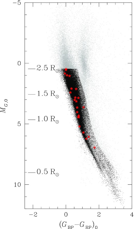
The MG, 0 versus (GBP − GRP)0 CMD of all the stars analysed in Paper II and in this work. Black points are the main-sequence stars with R⋆ ≤ 2.5R⊙, and grey points are the stars excluded from the analysis of candidate exoplanets’ frequency (see the text for details). For clarity, only 50 per cent of the stars are plotted. Red starred symbols indicate the positions on the CMD of the 23 candidate transiting exoplanets identified in stellar clusters from TESS data.
Because our candidate exoplanets orbit stars with R⋆ ≲ 2.5 R⊙, we first selected the light curves associated with these stars; we divided our sample of light curves on the basis of the TESS magnitude of the associated stars, considering bins of size ΔT = 1.0 in the magnitude range 6.0 ≤ T ≤ 18.0. In each bin, we randomly caught 350 light curves10 associated with stars having the previously estimated radii and masses, and, by using the routine INJECTTRANSIT implemented in vartools v.1.39 (Hartman & Bakos 2016), we injected in each light curve a periodic transit signal of a planet having radius |$R^{\rm inj}_{\rm P}$|, orbital period Pinj, random inclination iinj (with the constraint that there must be a transit), and eccentricity e = 0. We considered 12 different cases in which |$R^{\rm inj}_{\rm P}$| and Pinj randomly vary between a given minimum and a maximum; (i) we first injected (super-)Earth-size planets having radii |$0.85 \le R^{\rm inj}_{\rm P} \le 3.9R_{\rm Earth}$|; (ii) the second case we considered was for (super-)Neptune planets having radii |$3.9 \lt R^{\rm inj}_{\rm P} \le 11.2R_{\rm Earth} \sim 1 R_{\rm J}$|; finally, we considered giant planets with radii |$1.0 \lt R^{\rm inj}_{\rm P} \le 2.5R_{\rm J}$|. For each |$R^{\rm inj}_{\rm P}$| case, we considered random orbital periods in the following intervals: (a) short periods |$0.5 \le P^{\rm inj} \le 2.0\, {\rm d}$|; (b) short-medium periods |$2.0 \lt P^{\rm inj} \le 10.0\, {\rm d}$|; (c) long-medium periods |$10.0 \lt P^{\rm inj} \le 85.0\, {\rm d}$|; and (d) long periods |$85.0 \lt P^{\rm inj} \le 365.0\, {\rm d}$|. We have not made any selection on the time length of the light curves, so, on the basis of the associated star observability, the light curve can span randomly between ∼27 and ∼365 d.
We injected the transit signals in the raw light curves and we followed the same pipeline for the correction of the light curves and the detection of transit signals described in Sections 2 and 3. We considered the injected planet as recovered if it passes the selections illustrated in Section 3 and in Fig. 3 and if |$|P^{\rm inj}-P^{\rm inj}_{\rm TLS}|\lt 4.0\sigma (P^{\rm inj}_{\rm TLS})$|, where |$P^{\rm inj}_{\rm TLS}$| is the period obtained by the extraction of the TLS periodogram, and |$\sigma (P^{\rm inj}_{\rm TLS})$| its error. We also considered the planet as recovered if |$P^{\rm inj}_{\rm TLS}$| is equal to 0.5 × Pinj or 2.0 × Pinj, within |$4.0\sigma (P^{\rm inj}_{\rm TLS})$|. On a sample of 100 light curves selected randomly from those that passed the selections, we performed the vetting tests described in Section 311: all the selected objects passed the tests. We finally calculated the detection efficiency in each magnitude interval ΔT as the ratio Nrec/Ninj, where Nrec is the number of simulated planets recovered, and Ninj the number of light curves in which we injected transit signals. In Fig. 6 and Table 3, we reported the detection efficiency in the Pinj versus T grid for the three different planetary radius intervals: For Earth-size planets with RP ≲ 3.9REarth, the detection efficiency is low (|$\lesssim 40~{{\ \rm per\ cent}}$|), mainly because the large part of low-mass stars, for which the detection of small size planets is easier, is concentrated at magnitudes T ≳ 11 (see fig. 8 of Paper II); for short period Neptune-size planets (P < 10 d) orbiting stars with magnitude T ≲ 12, the detection efficiency is ≳30–|$50{{\ \rm per\ cent}}$|, and decreases at fainter magnitude to 20–30 per cent; we obtained a detection efficiency always |$\gtrsim 30~{{\ \rm per\ cent}}$| for giant planets with periods ≲10 d. For periods P ≳ 10 d, the detection efficiencies are always |$\lesssim 20~{{\ \rm per\ cent}}$|: This is an effect caused by the fact that only |$\sim 15{{\ \rm per\ cent}}$| of the stars in our sample are observed in more than two sectors, the detection of long-period planets difficult. Finally, even if we used different grids to flat the light curves to take into account the different kinds of variability, the detection efficiency can be lower for very active stars in young stellar clusters.
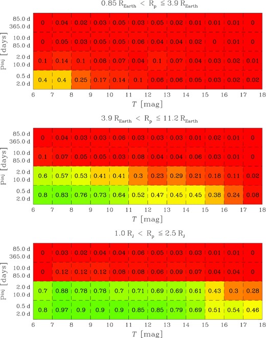
Transit detection efficiency (normalized to 1) of our pipeline in the injected period Pinj versus T magnitude plane for different size simulated planets: Earth and super-Earth-size planets (top panel), Neptune-size planets (middle panel), and Jupiter-size planets (bottom panel).
Detection efficiencies of the PATHOS pipeline.
| Detection efficiency ( per cent) | ||||
|---|---|---|---|---|
| 0.85 < RP ≤ 3.9REarth | ||||
| T | 0.5– | 2.0– | 10.0– | 85.0– |
| (mag) | 2.0 d | 10.0 d | 85.0 d | 365.0 d |
| 6–7 | 40.00 ± 23.66 | 10.00 ± 10.00 | <0.01 | <0.01 |
| 7–8 | 40.38 ± 7.38 | 14.42 ± 3.98 | 5.21 ± 2.39 | 3.85 ± 1.96 |
| 8–9 | 24.79 ± 3.64 | 10.26 ± 2.20 | 2.75 ± 1.14 | 2.14 ± 0.97 |
| 9–10 | 16.86 ± 2.37 | 8.00 ± 1.57 | 4.95 ± 1.27 | 2.86 ± 0.92 |
| 10–11 | 14.29 ± 2.16 | 7.43 ± 1.51 | 4.62 ± 1.22 | 4.86 ± 1.21 |
| 11–12 | 10.29 ± 1.80 | 4.29 ± 1.13 | 5.79 ± 1.37 | 3.43 ± 1.01 |
| 12–13 | 6.00 ± 1.35 | 9.71 ± 1.75 | 4.10 ± 1.16 | 4.57 ± 1.17 |
| 13–14 | 6.00 ± 1.35 | 6.57 ± 1.41 | 4.13 ± 1.17 | 2.00 ± 0.76 |
| 14–15 | 5.43 ± 1.28 | 4.29 ± 1.13 | 2.41 ± 0.92 | 1.14 ± 0.57 |
| 15–16 | 2.86 ± 0.92 | 3.14 ± 0.96 | 0.35 ± 0.35 | 1.43 ± 0.64 |
| 16–17 | 2.29 ± 0.82 | 2.00 ± 0.76 | 0.69 ± 0.49 | 0.86 ± 0.50 |
| 17–18 | 1.91 ± 0.97 | 0.96 ± 0.68 | <0.01 | <0.01 |
| 3.9 < RP ≤ 11.2REarth | ||||
| 6–7 | 80.00 ± 37.95 | 60.00 ± 30.98 | 10.00 ± 10.00 | <0.01 |
| 7–8 | 82.69 ± 12.05 | 56.73 ± 9.25 | 6.73 ± 2.63 | 3.85 ± 1.96 |
| 8–9 | 75.64 ± 7.54 | 52.56 ± 5.85 | 5.13 ± 1.52 | 2.56 ± 1.06 |
| 9–10 | 73.14 ± 6.02 | 40.57 ± 4.04 | 5.43 ± 1.28 | 3.14 ± 0.96 |
| 10–11 | 64.00 ± 5.48 | 40.86 ± 4.05 | 2.86 ± 0.92 | 5.71 ± 1.31 |
| 11–12 | 52.29 ± 4.77 | 30.37 ± 3.37 | 8.00 ± 1.57 | 3.43 ± 1.01 |
| 12–13 | 47.14 ± 4.45 | 22.57 ± 2.81 | 3.71 ± 1.05 | 2.86 ± 0.92 |
| 13–14 | 44.86 ± 4.31 | 28.57 ± 3.24 | 4.29 ± 1.13 | 3.43 ± 1.01 |
| 14–15 | 45.43 ± 4.34 | 21.14 ± 2.71 | 6.00 ± 1.35 | 1.14 ± 0.57 |
| 15–16 | 38.00 ± 3.87 | 18.29 ± 2.49 | 2.57 ± 0.87 | 2.00 ± 0.76 |
| 16–17 | 24.29 ± 2.94 | 11.43 ± 1.91 | 0.86 ± 0.50 | 1.43 ± 0.64 |
| 17–18 | 8.13 ± 2.05 | 1.91 ± 0.97 | <0.01 | <0.01 |
| 1.0 < RP ≤ 2.5RJ | ||||
| 6–7 | 80.00 ± 37.95 | 70.00 ± 34.50 | <0.01 | <0.01 |
| 7–8 | 97.12 ± 13.57 | 87.50 ± 12.56 | 11.54 ± 3.52 | 2.88 ± 1.69 |
| 8–9 | 90.17 ± 8.56 | 78.21 ± 7.72 | 11.54 ± 2.35 | 2.14 ± 0.97 |
| 9–10 | 90.00 ± 6.99 | 78.00 ± 6.30 | 12.29 ± 1.99 | 4.00 ± 1.09 |
| 10–11 | 90.00 ± 6.99 | 69.71 ± 5.81 | 7.71 ± 1.54 | 3.71 ± 1.05 |
| 11–12 | 84.57 ± 6.68 | 70.57 ± 5.86 | 8.29 ± 1.60 | 6.29 ± 1.38 |
| 12–13 | 85.14 ± 6.71 | 68.86 ± 5.76 | 6.29 ± 1.38 | 4.86 ± 1.21 |
| 13–14 | 78.86 ± 6.35 | 69.14 ± 5.78 | 8.57 ± 1.63 | 3.14 ± 0.96 |
| 14–15 | 69.43 ± 5.80 | 61.43 ± 5.32 | 6.57 ± 1.41 | 2.57 ± 0.87 |
| 15–16 | 51.14 ± 4.70 | 42.86 ± 4.18 | 3.71 ± 1.05 | 1.43 ± 0.64 |
| 16–17 | 53.71 ± 4.86 | 29.71 ± 3.32 | 3.71 ± 1.05 | 0.57 ± 0.41 |
| 17–18 | 46.41 ± 5.70 | 28.23 ± 4.16 | <0.01 | <0.01 |
4.2 FPP estimation
We used the tool vespa v. 0.612 (Morton 2012, 2015) to estimate the FPP in a Bayesian framework of each of the 23 candidate exoplanets previously selected. This software estimates the probability that the transit signal detected in a light curve is due to a real planet or to a different source. Different scenarios are taken into consideration to explain the signal: (i) simple eclipsing binary (EB, single/double period); (ii) a hierarchical triple system where two components eclipse (HEB, single/double period); (iii) a blended eclipsing binary inside the photometric aperture of the target (BEB, single/double period); and (iv) a transiting planet on the target star (pl). We want to highlight that vespa does not consider the scenario in which transit signals are due to non-astrophysical sources, even if in our case the probability it happens is low, because the analysed candidates passed a series of vetting tests that allow to exclude signals due to systematic effects. For each configuration, vespa simulates a representative stellar population, constrained by the information we have from the isochrone fitting and the light-curve modelling; in particular, we put constraints on the G, GBP, GRP, J2MASS, H2MASS, K2MASS magnitudes of the target star, the (α, δ) coordinates of the target, the effective temperature Teff, the density ρ⋆, and the surface gravity log (g) of the star, the orbital period P of the candidate exoplanet, the planet-to-star radius ratio RP/R⋆. Moreover, we gave as an input the light curve of the stars hosting the candidates. The software takes into account different false positive scenarios for those populations, and uses them to define a prior likelihood that a specific configuration actually exists and the likelihood of transit for those configurations. On the basis of the results obtained for different scenarios, at the end, it calculates the FPP that the transit signals are due to a false positive: The lower the FPP, the larger is the probability that the signal is due to a planet. We reported in Table 4 the FPPs and the most likely scenario (with the respective probability) derived with vespa for the 23 candidate exoplanets: ∼40 per cent of them have a probability ≳50 per cent to be a real exoplanet. It means that ∼3/5 of the signals we detected are likely false positives.
FPPs and most likely scenarios for PATHOS candidate exoplanets.
| TIC | PATHOS | FPP | Scenario (prob.) | FPPc | RUWE |
|---|---|---|---|---|---|
| Southern ecliptic hemisphere | |||||
| 0039291805 | 3 | 0.92 | BEB (0.51) | 0.87 | 1.023 |
| 0088977253 | 6 | 0.76 | EB (0.47) | 0.72 | 1.079 |
| 0125414447 | 9 | 0.98 | BEB (0.79) | 0.93 | 0.929 |
| 0126600730 | 10 | 0.97 | BEB (0.97) | 0.92 | 0.971 |
| 0159059181 | 16 | 0.99 | BEB (0.52) | 0.94 | 1.230 |
| 0306385801 | 20 | 0.51 | EB (0.51) | 0.48 | 0.851 |
| 0308538095 | 21 | 0.00 | pl (1.00) | 0.00 | 0.895 |
| 0372913337 | 23 | 0.74 | BEB (0.73) | 0.70 | 1.133 |
| 0410450228 | 25 | 0.46 | pl (0.54) | 0.44 | 0.901 |
| 0432564189 | 28 | 0.96 | BEB (0.92) | 0.91 | 1.078 |
| 0460205581 | 30 | 0.21 | pl (0.79) | 0.20 | 0.985 |
| 0460950389 | 31 | 0.22 | pl (0.78) | 0.21 | 0.891 |
| 0748919024 | 33 | 0.00 | pl (1.00) | 0.00 | 2.638 |
| 1036769612 | 34 | 0.63 | BEB (0.63) | 0.60 | 1.062 |
| Northern ecliptic hemisphere | |||||
| 0051022999 | 48 | 0.95 | BEB (0.88) | 0.90 | 0.947 |
| 0065557265 | 49 | 1.00 | BEB (0.41) | 0.95 | 1.066 |
| 0067424670 | 50 | 0.53 | pl (0.47) | 0.50 | 0.989 |
| 0185779182 | 53 | 0.36 | pl (0.64) | 0.34 | 1.086 |
| 0270618239 | 59 | 0.28 | pl (0.72) | 0.27 | 1.226 |
| 0298292983 | 63 | 1.00 | EB (0.67) | 0.95 | 1.112 |
| 0323717669 | 65 | 0.98 | BEB (0.96) | 0.93 | 1.893 |
| 0420288086 | 75 | 0.00 | pl (1.00) | 0.00 | 0.971 |
| 0421630760 | 76 | 1.00 | BEB (0.93) | 0.95 | 1.029 |
To test the reliability of the FPP estimation performed by vespa, we used this tool to validate 10 simulated transiting exoplanets extracted randomly from the sample of the recovered candidates described in Section 4.1 (considering all the scenarios). We ran vespa on the simulated exoplanets following the same procedure we adopted for the real candidate exoplanets. In an ideal case, the sum of all the FPPs obtained for the simulated exoplanets is equal to 0, but we obtained that ∑FPPi ∼ 0.5 ; it means that, on average, the measured FPP is overestimated of |$\sim 5~{{\ \rm per\ cent}}$|. We used this result to correct the FPPs measured for the real candidate exoplanets, as reported in Table 4 (FPPc).
We also reported in Table 4 the Renormalized Unit Weight Error (RUWE) index calculated as described by Belokurov et al. (2020); its value is ∼1 for sources that can be fitted with single-star models, and its value is larger (≳1.4) if the astrometric fit of the source by using single-star model is not the best solution. Among the candidates labelled as ‘pl’, only PATHOS-33 shows a high RUWE value (∼2.6), even if the FPP obtained with vespa is ∼0.
4.3 Candidate exoplanets’ frequency in open clusters
Candidate exoplanets’ frequencies.
| 0.85 < RP ≤ 3.9REarth | 3.9 < RP ≤ 11.2REarth | 1.0 < RP ≤ 2.5RJ | |||||||
|---|---|---|---|---|---|---|---|---|---|
| Period | |$f^{\rm min}_{\star }$| | |$f^{\rm mid}_{\star }$| | |$f^{\rm max}_{\star }$| | |$f^{\rm min}_{\star }$| | |$f^{\rm mid}_{\star }$| | |$f^{\rm max}_{\star }$| | |$f^{\rm min}_{\star }$| | |$f^{\rm mid}_{\star }$| | |$f^{\rm max}_{\star }$| |
| (d) | (per cent) | (per cent) | (per cent) | (per cent) | (per cent) | (per cent) | (per cent) | (per cent) | (per cent) |
| 0.5–2.0 | <0.034 | <0.063 | <0.086 | <0.004 | <0.007 | <0.009 | <0.002 | <0.004 | <0.006 |
| 2.0–10.0 | <0.092 | <0.191 | <0.269 | 0.034 ± 0.025 | 0.070 ± 0.052 | 0.098 ± 0.073 | 0.023 ± 0.013 | 0.047 ± 0.027 | 0.066 ± 0.038 |
| 10.0–85.0 | <0.533 | <1.505 | <2.218 | <0.327 | <0.925 | <1.364 | 0.555 ± 0.336 | 1.568 ± 0.955 | 2.312 ± 1.413 |
| 85.0–365.0 | <2.716 | <5.200 | <7.174 | <2.197 | <4.205 | <5.806 | <2.102 | <4.022 | <5.553 |
4.4 Age–planetary radius distribution
Fig. 7 shows the stellar age versus planetary radius distribution for the candidate transiting exoplanets in open clusters identified in this work and in Papers II, and reported as ‘pl’ in Table 4, and the candidates around stars in young associations identified in Paper III; the colours indicate the insolation flux S calculated on the basis of the stellar radius and effective temperature and of the planetary semimajor axis. Moreover, we included confirmed and candidate exoplanets from literature, orbiting stars in stellar clusters and associations, i.e. with a well-constrained age (coloured triangles). The list of literature objects plotted in Fig. 7 and the corresponding references are reported in Table 6. Finally, we also added objects (coloured squares, Nardiello et al. in preparation) that are under investigation in the context of the ‘GAPS Young Objects’ (GAPS-YO) project (Carleo et al. 2020), aimed at the monitoring of young and intermediate-age stars for the discovery and characterization of young planets. All the objects showed in Fig. 7 have orbital periods <100 d, i.e semimajor axis a ≲ 0.5 au.
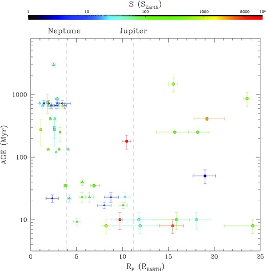
Stellar age versus planetary radius RP for candidate exoplanets identified in Papers II, III, and in this work (circles), for candidates and confirmed exoplanets from literature (triangles), and for the objects under investigation in the GAPS-YO programme (squares). Coloured points represent the exoplanets orbiting stars with well-constrained ages (from isochrone fitting and/or gyrochronological analysis of cluster/association members that host the stars). Different colours are associated with different insolation fluxes on the basis of the bar shown on the top.
Confirmed and candidate transiting exoplanets from literature.
| Object | Cluster/association | Age | Period | RP | Reference | Object | Cluster/association | Age | Period | RP | Reference |
|---|---|---|---|---|---|---|---|---|---|---|---|
| (Myr) | (d) | (REarth) | (Myr) | (d) | (REarth) | ||||||
| K-66b | NGC 6811 | |$863 ^{+30 }_{-30 }$| | |$17.815\,815 ^{+0.000\,075}_{-0.000\,075}$| | |$2.80^{+0.16}_{-0.16}$| | Meibom et al. (2013) | K2-33b | Upp-Sco | |$9.3^{+1.1}_{-1.1}$| | |$5.424\,865 ^{+0.000\,035 }_{-0.000\,031}$| | |$5.04 ^{+0.34}_{-0.37}$| | Mann et al. (2016a) |
| K-67b | NGC 6811 | |$863 ^{+30 }_{-30 }$| | |$15.725\,90 ^{+0.000\,11 }_{-0.000\,11 }$| | |$2.94^{+0.16}_{-0.16}$| | Meibom et al. (2013) | TOI-200b | Tuc-Hor | |$40 ^{+5 }_{-5 }$| | |$8.1387 ^{+0.0005 }_{-0.0005 }$| | |$5.63 ^{+0.22}_{-0.21}$| | Benatti et al. (2019) |
| HD 283869b | Hyades | |$728 ^{+71 }_{-71 }$| | |$106 ^{+74.0 }_{-25.0 }$| | |$1.96^{+0.13}_{-0.16}$| | Vanderburg et al. (2018) | TOI-451b | Psc-Eri | |$134^{+6.5}_{-6.5}$| | |$1.858\,703^{+0.000\,025}_{-0.000\,035}$| | |$1.91^{+0.12}_{-0.12}$| | Newton et al. (2021) |
| K2-25b | Hyades | |$728 ^{+71 }_{-71 }$| | |$3.484\,552 ^{+0.000\,031}_{-0.000\,037}$| | |$3.43^{+0.95}_{-0.31}$| | Mann et al. (2016b) | TOI-451c | Psc-Eri | |$134^{+6.5}_{-6.5}$| | |$9.192\,522^{+0.000\,06}_{-0.000\,10}$| | |$3.10^{+0.13}_{-0.13}$| | Newton et al. (2021) |
| K2-136Ab | Hyades | |$728 ^{+71 }_{-71 }$| | |$7.975\,292 ^{+0.000\,833}_{-0.000\,770}$| | |$0.99^{+0.06}_{-0.04}$| | Mann et al. (2018) | TOI-451d | Psc-Eri | |$134^{+6.5}_{-6.5}$| | |$16.364\,988^{+0.000\,44}_{-0.000\,044}$| | |$4.07^{+0.15}_{-0.15}$| | Newton et al. (2021) |
| K2-136Ac | Hyades | |$728 ^{+71 }_{-71 }$| | |$17.307\,137 ^{+0.000\,252}_{-0.000\,284}$| | |$2.91^{+0.11}_{-0.10}$| | Mann et al. (2018) | TOI-1098b | Melange-1 | |$250^{+50}_{-70}$| | |$10.182\,71^{+0.0004}_{-0.000\,04}$| | |$3.2^{+0.1}_{-0.1}$| | Tofflemire et al. (2021) |
| K2-136Ad | Hyades | |$728 ^{+71 }_{-71 }$| | |$25.575\,065 ^{+0.002\,418}_{-0.002\,357}$| | |$1.45^{+0.11}_{-0.08}$| | Mann et al. (2018) | HD 63433b | UMa | |$414^{+23 }_{-23}$| | |$7.108\,01 ^{+0.000\,46 }_{-0.000\,34 }$| | |$2.15 ^{+0.10}_{-0.10}$| | Mann et al. (2020) |
| K2-95b | Praesepe | |$670 ^{+67 }_{-67 }$| | |$10.135\,091 ^{+0.000\,495}_{-0.000\,488}$| | |$3.7 ^{+0.2 }_{-0.2 }$| | Mann et al. (2017) | HD 63433c | UMa | |$414^{+23 }_{-23}$| | |$20.5455 ^{+0.0011 }_{-0.0011 }$| | |$2.64 ^{+0.12}_{-0.12}$| | Mann et al. (2020) |
| K2-100b | Praesepe | |$670 ^{+67 }_{-67 }$| | |$1.673\,915 ^{+0.000\,011}_{-0.000\,011}$| | |$3.5 ^{+0.2 }_{-0.2 }$| | Mann et al. (2017) | HIP 67522b | Sco-Cen | |$17 ^{+2 }_{-2 }$| | |$6.959\,503 ^{+0.000\,016 }_{-0.000\,015}$| | |$10.07 ^{+0.47}_{-0.47}$| | Rizzuto et al. (2020) |
| K2-101b | Praesepe | |$670 ^{+67 }_{-67 }$| | |$14.677\,303 ^{+0.000\,824}_{-0.000\,809}$| | |$3.0 ^{+0.1 }_{-0.1 }$| | Mann et al. (2017) | HIP 67522c | Sco-Cen | |$17 ^{+2 }_{-2 }$| | |$54.0 ^{+70.0 }_{-24.0 }$| | |$8.01 ^{+0.75}_{-0.71}$| | Rizzuto et al. (2020) |
| K2-102b | Praesepe | |$670 ^{+67 }_{-67 }$| | |$9.915\,651 ^{+0.001\,194}_{-0.001\,175}$| | |$1.3 ^{+0.1 }_{-0.1 }$| | Mann et al. (2017) | AU Mic b | AU Mic | |$22 ^{+3 }_{-3 }$| | |$8.463\,21 ^{+0.000\,04 }_{-0.000\,04 }$| | |$4.20 ^{+0.20}_{-0.20}$| | Plavchan et al. (2020) |
| K2-103b | Praesepe | |$670 ^{+67 }_{-67 }$| | |$21.169\,687 ^{+0.001\,636}_{-0.001\,655}$| | |$2.2 ^{+0.2 }_{-0.1 }$| | Mann et al. (2017) | AU Mic c | AU Mic | |$22 ^{+3 }_{-3 }$| | |$30.0 ^{+6.0 }_{-6.0 }$| | |$2.35 ^{+0.67}_{-0.67}$| | Plavchan et al. (2020) |
| K2-104b | Praesepe | |$670 ^{+67 }_{-67 }$| | |$1.974\,189 ^{+0.000\,110}_{-0.000\,109}$| | |$1.9 ^{+0.2 }_{-0.1 }$| | Mann et al. (2017) | V 1298c | Tau | |$23 ^{+4 }_{-4 }$| | |$8.249\,58 ^{+0.000\,72 }_{-0.000\,72 }$| | |$5.59 ^{+0.36}_{-0.32}$| | David et al. (2019) |
| K2-264b | Praesepe | |$670 ^{+67 }_{-67 }$| | |$5.839\,770 ^{+0.000\,063}_{-0.000\,063}$| | |$2.27^{+0.20}_{-0.16}$| | Rizzuto et al. (2018) | V 1298d | Tau | |$23 ^{+4 }_{-4 }$| | |$12.4032 ^{+0.0015 }_{-0.0015 }$| | |$6.41 ^{+0.45}_{-0.40}$| | David et al. (2019) |
| K2-264c | Praesepe | |$670 ^{+67 }_{-67 }$| | |$19.663\,650 ^{+0.000\,303}_{-0.000\,306}$| | |$2.77^{+0.20}_{-0.18}$| | Rizzuto et al. (2018) | V 1298b | Tau | |$23 ^{+4 }_{-4 }$| | |$24.1396 ^{+0.0018 }_{-0.0018 }$| | |$10.27 ^{+0.58}_{-0.53}$| | David et al. (2019) |
| K2-231b | Ruprecht 147 | |$3000^{+250 }_{-250}$| | |$13.841\,901 ^{+0.001\,352}_{-0.001\,352}$| | |$2.5 ^{+0.2 }_{-0.2 }$| | Curtis et al. (2018) | V 1298e | Tau | |$23 ^{+4 }_{-4 }$| | |$60 ^{+60 }_{-18 }$| | |$8.74 ^{+0.84}_{-0.72}$| | David et al. (2019) |
| K2-284b | Cas-Tau | |$120^{+640}_{-20}$| | |$4.795\,07 ^{+0.000\,12 }_{-0.000\,12 }$| | |$2.77 ^{+0.12}_{-0.12}$| | David et al. (2018) |
We found that Jupiters with RP ≳ 1RJ are distributed randomly between ∼10 Myr and ∼10 Gyr. Objects having Neptune-sizes or smaller (Earths/super-Earths) are concentrated at ages >200–300 Myr; anyway the lack of this kind of objects around young stars might be an observational bias due to the difficulty of detecting their transits in the highly variable light curves of active young stars. Objects having a planetary radius |$4 \lesssim R_{\rm P} \lesssim 10R_{\rm Earth}$| are concentrated at ages <100–200 Myr. Is it an observational bias, or the lack of super-Neptune/sub-Jovian-size planets orbiting (on short periods) stars with (well-measured) ages ≳200 Myr is due to an evolutionary effect of the planets?
The majority of low-mass close-in exoplanets (with RP= 1–4REarth) detected until today orbit field stars with ages ≳1–3 Gyr. Some of these planets are almost totally rocky (e.g. Kepler-93; Dressing et al. 2015), others have low densities that can be explained by the presence of an extended H/He atmosphere. Among them, the Kepler-36 system is particular because formed by two planets with very similar semimajor axis, but totally different densities (Carter et al. 2012), with the inner planet less massive than the external planet. Lopez & Fortney (2013) proved that both the exoplanets in the Kepler-36 system were born with H/He atmospheres and were more massive in the early stages of their life, and that, given the lower core mass of the inner planet, the latter has lost large part of its atmosphere, despite the outer planet that was able to retain about half of its initial atmosphere. As explained in detail in the review by Owen (2019, see also references therein), there is strong evidence that atmospheric escape is the mechanism that prevails in the first stages of a low-mass close-in exoplanet’s evolution, and it depends (in a first approximation) on the characteristics of the host star (and its high-energy emissions), the distance of the planet from the star, and its core mass. During their formation, these planets accreted large amount of H/He into their expanded atmospheres, inflating their radius at 5–13REarth; in few hundreds Myr, if irradiated strongly enough, these planets lose the large part of their atmosphere, resulting in (super-)Earth/sub-Neptune-size planets (Owen et al. 2020). Even if Fig. 7 does not show any particular dependence on the insolation flux, the distribution of short-period (candidate) exoplanets with radii |$1 13 \lesssim R_{\rm P}\lesssim 13R_{\rm Earth}$| seems to confirm the idea of atmospheric escape on timescales of ≲100–200 Myr; anyway, as demonstrated by Owen (2020), even if challenging, for many of these candidates, mass measurements are mandatory in order to understand the mechanisms and constraint the time-scales of planetary atmospheric evolution.
Other possible explanations for the lack of planets older than ∼200 Myr in the interval 4 ≲ RP ≲ 10REarth may be linked to the dynamical evolution of this kind of planets after their formation, such as migration due to interaction with the protoplanetary disc or planet-planet scattering (Fabrycky & Tremaine 2007; Chatterjee et al. 2008; Kley & Nelson 2012). These phenomena are expected to modify the orbital characteristics of the planets, such as inclination, eccentricity, and semimajor axis, making the detection of a possible transit of these planets more difficult. These phenomena occur on scales of a few tens of Myr or less, and may not yet have come into play for the objects reported in this analysis.
5 SUMMARY AND CONCLUSION
The aim of the PATHOS project is the discovery and first characterization of transiting objects around stars in stellar clusters and associations observed by TESS. Stellar clusters and associations offer the rare opportunity to obtain precise measurements of the ages of the stars (usually affected by large uncertainties), in addition to stars’ physical parameters such as radius, mass, effective temperature, etc., and analyse planet characteristics as a function of its host’s properties. Because of the low resolution of TESS cameras, stellar clusters appear as very crowded regions on FFIs, and appropriate tools are necessary to obtain high-precision light curves for cluster members. In order to obtain the best light curves, we developed a cutting-edge technique for the extraction of high-precision photometry of stars in crowded fields, based on the use of empirical PSFs and neighbour subtraction, that allows us to minimize neighbour contamination and extract light curves for very faint objects.
In this work, the fourth of the PATHOS series, we extracted and corrected 150 216 light curves of 89 858 open cluster members listed in the Cantat-Gaudin et al. (2018)’s catalogue and observed during the Cycle 2 (Sectors 14–26) of the TESS mission. By using the pipeline already tested in the previous papers of the series, we searched for transit signals among the light curves, finding 39 transiting objects of interest, which are added to the 33 objects orbiting open cluster members identified in Paper II. We modelled their light curves to extract planet parameters. From the two lists of objects of interest, we isolated 23 candidates with planetary radius |$R_{\rm P} \lesssim 2.5R_{\rm J}$|, and we calculated their FPPs to be a planet, finding that about 3/5 of them are likely false positives.
Taking into account of the transit detection efficiency of our pipeline and of the rate of false positives, we calculated the frequencies of candidate exoplanets in open clusters (f⋆) for different (Earth/Neptune/Jupiter) sizes planets in different orbital periods intervals (between 0.5 and 365 d). Because we did not detect any strong candidate with orbital period <2 d, we calculated the frequency upper limit, finding f⋆ ≲ 0.06, ≲ 0.007, and ≲0.004 per cent for Earth-, Neptune-, and Jupiter-size candidate exoplanets, respectively. For candidate exoplanets with periods 2.0 < P < 10.0 d, we found for Earth-size objects, an upper limit f⋆ ≲ 0.2 per cent, while for candidate planets with RP ≳ 3.9REarth, the frequency is ∼0.06 per cent; in the range 10.0 < P < 85.0 d, we obtained that the frequency of Earth and Neptune-size candidates is |$\lesssim 2.~{{\ \rm per\ cent}}$|, while the measured frequency for giant planets is |$\sim 1.6~{{\ \rm per\ cent}}$|; finally, for long period planets (>85 d), we found that the frequency of candidate exoplanets is |$\lt 5\!-\!7~{{\ \rm per\ cent}}$|. The large part of the measured and upper limit frequencies are lower than the values reported by Fressin et al. (2013) in the same period intervals for the corresponding size exoplanets around field stars (even if bias can be introduced by the poor statistic of our sample); an exception are the giant planets with 10–85 d period: We found a mean frequency of 1.6 ± 0.9 per cent, in agreement with the value obtained by Fressin et al. (2013, |$1.5 \pm 0.2~{{\ \rm per\ cent}}$|), but also by Santerne et al. (2016, f⋆ = 0.90 ± 0.26 per cent) and Deleuil et al. (2018, f⋆ = 1.86 ± 0.68 per cent).
We investigated the stellar age versus planetary radius distribution by using the results obtained in the PATHOS project and the results obtained in other works for exoplanets orbiting stars with well constrained ages. We only used planets with orbital periods <100 d and we divided the distribution on the basis of the planetary radius RP: (1) for (candidate) exoplanets with RP ≳ 1RJ, we found no particular trends, and the planets are randomly distributed on over the range of ages; (2) objects with RP ≲ 4REarth are concentrated at ages >100–200 Myr, but it might be an observational bias due to the difficulty to detect (super-)Earth transits in the light curve of young active stars; and (3) in the range |$4 \lesssim R_{\rm P} \lesssim 13R_{\rm Earth}$|, there is a concentration of objects around young stars with ages <100 Myr. A possible explanation of such concentration is that these objects are young planets with rocky cores that, in the early stages of their formation, have accreted large amount of hydrogen and helium in their atmospheres, inflating their radius. On the time-scales of ∼100–200 Myr, they lose large part of their atmosphere mainly because of the strong irradiation of the host star (see Owen 2019 for a review of all the mechanisms that contribute to the atmosphere escape), and within few hundreds Myr, their radius decreases to that typical of (super-)Earth/Neptune planets. Other explanations can be related to the dynamical evolution of these exoplanets (planet-planet scattering, migration, etc.).
For this reason, the analysis of light curves of members of young associations (ages ≲200–300 Myr), the subject of the next PATHOS works, will be essential to shed light on the mechanisms of planet formation and evolution of close-in sub-Jovian planets.
SUPPORTING INFORMATION
Supplementary data are available at https://archive.stsci.edu/hlsp/pathos online.
Please note: Oxford University Press is not responsible for the content or functionality of any supporting materials supplied by the authors. Any queries (other than missing material) should be directed to the corresponding author for the article.
ACKNOWLEDGEMENTS
DN acknowledges the support from the French Centre National d’Etudes Spatiales (CNES). GL acknowledges support by CARIPARO Foundation, according to the agreement CARIPARO-Università degli Studi di Padova (Pratica n. 2018/0098). LB acknowledges the funding support from Italian Space Agency (ASI) regulated by ‘Accordo ASI-INAF n. 2013-016-R.0 del 9 luglio 2013 e integrazione del 9 luglio 2015 CHEOPS Fasi A/B/C’. The authors thank the anonymous referee for carefully reading this paper and for the useful suggestions that improved this work. This paper includes data collected by the TESS mission. Funding for the TESS mission is provided by the NASA Explorer Program. This work has made use of data from the European Space Agency (ESA) mission Gaia (https://www.cosmos.esa.int/gaia), processed by the Gaia Data Processing and Analysis Consortium (DPAC; https://www.cosmos.esa.int/web/gaia/dpac/consortium). Funding for the DPAC has been provided by national institutions, in particular the institutions participating in the Gaia Multilateral Agreement. Some tasks of the data analysis have been carried out using vartools v 1.39 (Hartman & Bakos 2016) and tlspython routine (Hippke & Heller 2019).
DATA AVAILABILITY
The data underlying this paper are available in MAST at doi:10.17909/t9-es7m-vw14 and https://archive.stsci.edu/hlsp/pathos.
Footnotes
As also shown in Fig. 1, during Sectors 14–16 and 24–26, the TESS pointings were modified in order to avoid excessive contamination by stray Earth- and Moon-light in cameras 1 and 2.
tls v. 1.0.24; https://github.com/hippke/tls.
In such crowded environments, the completeness of the Gaia DR2 catalogue is ≳80–90 per cent for stars with 16 ≲ G ≲ 18 and |$\gtrsim 95\, {{\ \rm per\ cent}}$| for brighter stars (see Gaia DR2 Documentation release 1.2, Section 10.7.4), and therefore the values of dilution factor obtained in this work represent, within the errors, a good estimate of the real dilution factor. In the case of close binaries with separation <1–2 arcsec, Ziegler et al. (2018) demonstrated that Gaia satellite is not always able to resolve the components. If two (or more stars) are not resolved by Gaia, the result will be a single source whose flux will approximately be equal to the sum of the fluxes coming from the different not-resolved components; this does not affect the subtraction process in the extraction of the light curve because we have considered the multiple components as a single source whose flux is the sum of components’ fluxes. It might affect the estimate of the dilution factor used for the modelling of the transits, and, for this reason, further AO follow-up of the candidates are mandatory.
If the number of light curves in the considered magnitude bin was <350, we considered all the light curves belonging to that bin.
The analysis of the centroid was excluded from these vetting tests because it is obtained analysing the images, where there are no signals for the simulated transits.
REFERENCES
APPENDIX A: LIGHT-CURVE MODELLING
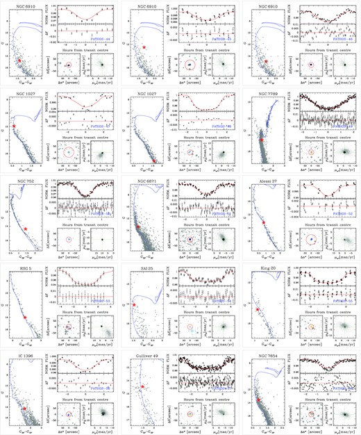
Overview on the candidate exoplanets PATHOS-44–PATHOS-58. On the left-hand, the G versus GBP − GRP CMD of the cluster that hosts the target star (red star or dashed line when GBP − GRP colour is not available) and the isochrone (blue) fitted with the cluster parameters listed in Table 1. The top right-hand panel shows the folded light curve (grey points) of the candidate and the model (in red) found with pyorbit; the middle panel shows the difference between the observed points and the model. The bottom left-hand panel shows the 95 × 95 arcsec2 finding chart centred on the target star; red circle is the aperture adopted to extract photometry, crosses are the in-/out-of-transit difference centroid. The bottom right-hand panel shows the vector-point diagram, centred on the target star, for all the stars that are within 10 arcmin from the target star; black points are the cluster members listed in the catalogue by Cantat-Gaudin et al. (2018).
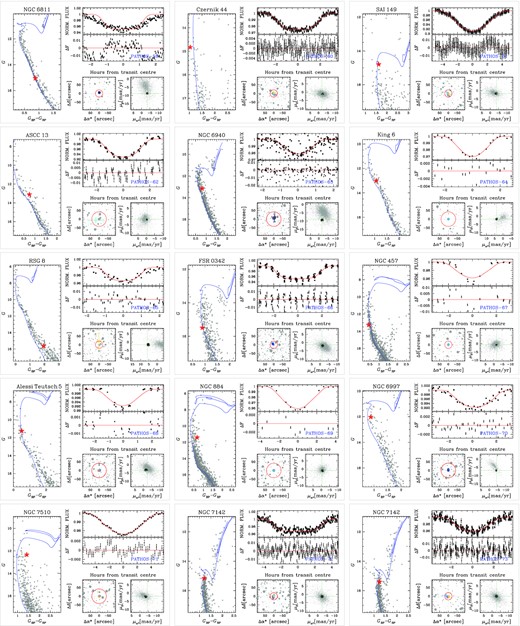
As in Fig. A1, but for PATHOS-59–PATHOS-73.
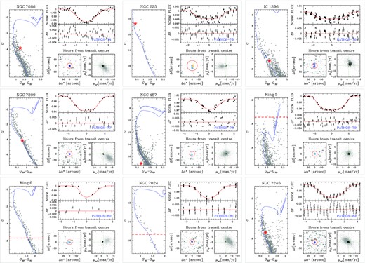
As in Fig. A1, but for PATHOS-74–PATHOS-82.
Star parameters and priors for the modelling.
| TIC | PATHOS | Cluster | α | δ | T | R⋆ | M⋆ | Period | T0 | LDc1 | LDc2 | df |
|---|---|---|---|---|---|---|---|---|---|---|---|---|
| (°) | (°) | (mag) | (R⊙) | (M⊙) | (d) | (BTJD) | ||||||
| 0013416465 | 44 | NGC 6910 | 305.4104 | 40.6532 | 14.0 | 1.88 ± 0.05 | 2.74 ± 0.05 | |$\mathcal {U}(5.5, 6.0)$| | |$\mathcal {U}(1688, 1689)$| | 0.15 ± 0.10 | 0.18 ± 0.10 | 0.02 ± 0.05 |
| 0013866376 | 45 | NGC 6910 | 305.6858 | 40.5015 | 11.6 | 3.68 ± 0.08 | 5.90 ± 0.19 | |$\mathcal {U}(9, 9.5)$| | |$\mathcal {U}(1686.0, 1687.0)$| | 0.06 ± 0.10 | 0.10 ± 0.10 | 0.04 ± 0.01 |
| 0013875852 | 46 | NGC 6910 | 305.7604 | 40.9818 | 13.9 | 1.84 ± 0.05 | 2.64 ± 0.05 | |$\mathcal {U}(8.0, 8.5)$| | |$\mathcal {U}(1683.5, 1684.5)$| | 0.15 ± 0.10 | 0.18 ± 0.10 | 0.14 ± 0.05 |
| 0050361536 | 47 | NGC 1027 | 40.4690 | 61.7671 | 11.6 | 2.64 ± 0.12 | 2.58 ± 0.07 | |$\mathcal {U}(12.6, 13.4)$| | |$\mathcal {U}(1793, 1794)$| | 0.15 ± 0.10 | 0.20 ± 0.10 | 0.01 ± 0.05 |
| 0051022999 | 48 | NGC 1027 | 41.9287 | 61.6554 | 16.2 | 0.80 ± 0.03 | 0.89 ± 0.00 | |$\mathcal {U}(7.5, 8.0)$| | |$\mathcal {U}(1794.0, 1795.0)$| | 0.37 ± 0.10 | 0.33 ± 0.10 | 0.92 ± 0.05 |
| 0065557265 | 49 | NGC 7789 | 359.1359 | 57.0475 | 14.0 | 2.06 ± 0.67 | 1.54 ± 0.03 | |$\mathcal {U}(1.5, 2.0)$| | |$\mathcal {U}(1785.2, 1785.5)$| | 0.28 ± 0.10 | 0.28 ± 0.10 | 0.01 ± 0.05 |
| 0067424670 | 50 | NGC 752 | 29.0476 | 37.9182 | 13.6 | 0.76 ± 0.03 | 0.83 ± 0.05 | |$\mathcal {U}(0.9, 1.3)$| | |$\mathcal {U}(1790.5, 1791.5)$| | 0.39 ± 0.10 | 0.35 ± 0.10 | 0.08 ± 0.05 |
| 0106235729 | 51 | NGC 6871 | 301.0821 | 35.7889 | 13.0 | 2.01 ± 0.04 | 3.16 ± 0.06 | |$\mathcal {U}(3.7,4.3)$| | |$\mathcal {U}(1684, 1685)$| | 0.13 ± 0.10 | 0.16 ± 0.10 | 0.03 ± 0.05 |
| 0154304816 | 52 | Alessi 37 | 342.4106 | 46.3500 | 12.7 | 1.35 ± 0.03 | 1.39 ± 0.05 | |$\mathcal {U}(3.5, 4.0)$| | |$\mathcal {U}(1742.0, 1743.0)$| | 0.27 ± 0.10 | 0.28 ± 0.10 | 0.02 ± 0.05 |
| 0185779182 | 53 | RSG 5 | 302.5300 | 45.0274 | 13.3 | 0.76 ± 0.05 | 0.77 ± 0.07 | |$\mathcal {U}(0.1,99)$| | |$\mathcal {U}(1711, 1712)$| | 0.42 ± 0.10 | 0.36 ± 0.10 | 0.02 ± 0.03 |
| 0251494772 | 54 | SAI 25 | 45.3145 | 57.1103 | 13.3 | 4.42 ± 0.35 | 3.39 ± 0.16 | |$\mathcal {U}(5.0, 5.5)$| | |$\mathcal {U}(1795, 1796)$| | 0.15 ± 0.10 | 0.19 ± 0.10 | 0.01 ± 0.05 |
| 0251975224 | 55 | King 20 | 353.1928 | 58.3744 | 14.0 | 1.49 ± 0.04 | 1.57 ± 0.06 | |$\mathcal {U}(3.3, 3.9)$| | |$\mathcal {U}(1956, 1957)$| | 0.23 ± 0.10 | 0.26 ± 0.10 | 0.04 ± 0.02 |
| 0260167199 | 56 | IC 1396 | 325.3457 | 57.1089 | 13.5 | 1.43 ± 0.03 | 1.34 ± 0.05 | |$\mathcal {U}(17.3, 18.0)$| | |$\mathcal {U}(1741.0, 1742.0)$| | 0.33 ± 0.10 | 0.31 ± 0.10 | 0.10 ± 0.05 |
| 0269519402 | 57 | Gulliver 49 | 350.6974 | 61.9366 | 13.7 | 2.54 ± 0.07 | 2.93 ± 0.07 | |$\mathcal {U}(3.0, 3.5)$| | |$\mathcal {U}(1806.0, 1806.5)$| | 0.15 ± 0.10 | 0.18 ± 0.10 | 0.12 ± 0.05 |
| 0270022396 | 58 | NGC 7654 | 351.2741 | 61.6596 | 13.1 | 2.00 ± 0.05 | 2.76 ± 0.06 | |$\mathcal {U}(3.6, 3.9)$| | |$\mathcal {U}(1807.3, 1807.5)$| | 0.15 ± 0.10 | 0.18 ± 0.10 | 0.18 ± 0.05 |
| 0270618239 | 59 | NGC 6811 | 293.6701 | 46.2956 | 14.5 | 0.99 ± 0.03 | 1.07 ± 0.05 | |$\mathcal {U}(2.2, 3.0)$| | |$\mathcal {U}(1683.0, 1684.0)$| | 0.32 ± 0.30 | 0.30 ± 0.30 | 0.05 ± 0.05 |
| 0270920839 | 60 | Czernik 44 | 353.5841 | 62.0029 | 14.3 | 3.94 ± 0.09 | 6.30 ± 0.22 | |$\mathcal {U}(5.0, 5.5)$| | |$\mathcal {U}(1767.5, 1768.5)$| | 0.05 ± 0.10 | 0.08 ± 0.10 | 0.70 ± 0.05 |
| 0271443321 | 61 | SAI 149 | 354.4998 | 60.5393 | 13.9 | 5.00 ± 0.32 | 3.41 ± 0.17 | |$\mathcal {U}(5.7, 6.2)$| | |$\mathcal {U}(1765.0, 1766.0)$| | 0.15 ± 0.10 | 0.21 ± 0.10 | 0.04 ± 0.05 |
| 0285249796 | 62 | ASCC 13 | 78.2136 | 44.5317 | 12.7 | 1.49 ± 0.03 | 1.73 ± 0.05 | |$\mathcal {U}(4.5, 5.0)$| | |$\mathcal {U}(1816, 1817)$| | 0.20 ± 0.10 | 0.24 ± 0.10 | 0.31 ± 0.05 |
| 0298292983 | 63 | NGC 6940 | 308.6667 | 27.8038 | 12.7 | 1.67 ± 0.05 | 1.56 ± 0.05 | |$\mathcal {U}(1.2, 1.3)$| | |$\mathcal {U}(1700.9, 1701.2)$| | 0.24 ± 0.10 | 0.26 ± 0.10 | 0.13 ± 0.05 |
| 0316246231 | 64 | King 6 | 51.9527 | 56.5553 | 12.4 | 1.62 ± 0.03 | 1.77 ± 0.05 | |$\mathcal {U}(8.3, 8.7)$| | |$\mathcal {U}(1795.5, 1796.5)$| | 0.20 ± 0.10 | 0.24 ± 0.10 | 0.01 ± 0.05 |
| 0323717669 | 65 | RSG 8 | 348.0553 | 59.4878 | 14.6 | 0.64 ± 0.03 | 0.69 ± 0.05 | |$\mathcal {U}(4.0, 4.5)$| | |$\mathcal {U}(1955.0, 1956.0)$| | 0.45 ± 0.10 | 0.36 ± 0.10 | 0.70 ± 0.05 |
| 0326483210 | 66 | FSR 0342 | 331.8775 | 53.3684 | 15.0 | 1.83 ± 0.05 | 2.01 ± 0.07 | |$\mathcal {U}(3.5, 4.0)$| | |$\mathcal {U}(1741.0, 1742.0)$| | 0.17 ± 0.10 | 0.22 ± 0.10 | 0.57 ± 0.05 |
| 0332258412 | 67 | NGC 457 | 19.5199 | 58.7259 | 13.0 | 2.86 ± 0.06 | 4.93 ± 0.06 | |$\mathcal {U}(7.0, 7.5)$| | |$\mathcal {U}(1794.5, 1795.5)$| | 0.07 ± 0.10 | 0.12 ± 0.10 | 0.02 ± 0.05 |
| 0334949878 | 68 | Alessi Teutsch 5 | 331.7424 | 60.5581 | 11.0 | 2.38 ± 0.06 | 3.38 ± 0.05 | |$\mathcal {U}(19.0, 20.0)$| | |$\mathcal {U}(1741.0, 1742.0)$| | 0.13 ± 0.10 | 0.16 ± 0.10 | 0.01 ± 0.05 |
| 0348608380 | 69 | NGC 884 | 35.5582 | 57.3225 | 11.0 | 4.13 ± 0.08 | 7.63 ± 0.06 | |$\mathcal {U}(16, 99)$| | |$\mathcal {U}(1806.0, 1807.5)$| | 0.02 ± 0.10 | 0.01 ± 0.10 | 0.01 ± 0.05 |
| 0356973763 | 70 | NGC 6997 | 314.4065 | 44.5798 | 11.6 | 2.51 ± 0.15 | 2.24 ± 0.06 | |$\mathcal {U}(9.5, 10.3)$| | |$\mathcal {U}(1720, 1721)$| | 0.17 ± 0.10 | 0.22 ± 0.10 | 0.03 ± 0.05 |
| 0377619148 | 71 | NGC 7510 | 348.0732 | 60.4962 | 11.6 | 7.15 ± 0.46 | 6.77 ± 0.47 | |$\mathcal {U}(19.5, 20.0)$| | |$\mathcal {U}(1784, 1785)$| | 0.06 ± 0.10 | 0.11 ± 0.10 | 0.01 ± 0.05 |
| 0408094816 | 72 | NGC 7142 | 326.3290 | 65.7443 | 14.5 | 2.57 ± 0.26 | 1.64 ± 0.07 | |$\mathcal {U}(5.3,5.9)$| | |$\mathcal {U}(1743.5, 1744.5)$| | 0.28 ± 0.10 | 0.28 ± 0.10 | 0.04 ± 0.05 |
| 0408358709 | 73 | NGC 7142 | 326.6784 | 65.7431 | 14.7 | 2.17 ± 0.32 | 1.57 ± 0.06 | |$\mathcal {U}(6.0,6.5)$| | |$\mathcal {U}(1741.0, 1742.0)$| | 0.27 ± 0.10 | 0.28 ± 0.10 | 0.02 ± 0.05 |
| 0417058223 | 74 | NGC 7086 | 322.8993 | 51.7531 | 13.2 | 2.09 ± 0.05 | 2.76 ± 0.07 | |$\mathcal {U}(5.2, 5.8)$| | |$\mathcal {U}(1712.0, 1713.0)$| | 0.15 ± 0.10 | 0.18 ± 0.10 | 0.44 ± 0.05 |
| 0420288086 | 75 | NGC 225 | 10.9627 | 61.8356 | 10.4 | 2.20 ± 0.06 | 2.69 ± 0.06 | |$\mathcal {U}(6.3, 6.9)$| | |$\mathcal {U}(1769.0, 1770.0)$| | 0.15 ± 0.10 | 0.19 ± 0.10 | 0.01 ± 0.05 |
| 0421630760 | 76 | IC 1396 | 324.6780 | 57.8705 | 13.7 | 1.41 ± 0.03 | 1.32 ± 0.05 | |$\mathcal {U}(4.0, 4.5)$| | |$\mathcal {U}(1742.0, 1743.0)$| | 0.33 ± 0.10 | 0.32 ± 0.10 | 0.10 ± 0.05 |
| 0427943483 | 77 | NGC 7209 | 331.5198 | 46.8716 | 13.7 | 1.35 ± 0.03 | 1.37 ± 0.05 | |$\mathcal {U}(6.0, 6.5)$| | |$\mathcal {U}(1738, 1739)$| | 0.27 ± 0.10 | 0.28 ± 0.10 | 0.01 ± 0.05 |
| 0602870459 | 78 | NGC 457 | 19.2565 | 58.4526 | 16.7 | 1.37 ± 0.05 | 1.41 ± 0.07 | |$\mathcal {U}(3.0, 3.5)$| | |$\mathcal {U}(1792.5, 1793.5)$| | 0.27 ± 0.10 | 0.28 ± 0.10 | 0.95 ± 0.05 |
| 0645455722 | 79 | King 5 | 48.2841 | 52.2956 | 13.0 | 18.44 ± 0.58 | 1.98 ± 0.14 | |$\mathcal {U}(2.5, 3.0)$| | |$\mathcal {U}(1794.5, 1795.0)$| | 0.43 ± 0.30 | 0.38 ± 0.30 | 0.65 ± 0.05 |
| 0645713782 | 80 | King 6 | 52.1609 | 56.5984 | 15.2 | 0.94 ± 0.03 | 1.04 ± 0.05 | |$\mathcal {U}(6.3, 6.9)$| | |$\mathcal {U}(1790.5, 1791.5)$| | 0.32 ± 0.10 | 0.30 ± 0.10 | 0.75 ± 0.05 |
| 1961935435 | 81 | NGC 7024 | 316.4611 | 41.5474 | 14.9 | 1.35 ± 0.03 | 1.38 ± 0.05 | |$\mathcal {U}(2.5, 3.0)$| | |$\mathcal {U}(1713.0, 1714.0)$| | 0.27 ± 0.10 | 0.28 ± 0.10 | 0.78 ± 0.05 |
| 2015243161 | 82 | NGC 7245 | 333.8243 | 54.2961 | 14.9 | 1.85 ± 0.05 | 2.06 ± 0.07 | |$\mathcal {U}(11.2, 11.8)$| | |$\mathcal {U}(1745.5, 1746.5)$| | 0.17 ± 0.10 | 0.22 ± 0.10 | 0.46 ± 0.05 |
