


ABSTRACT
We examine four high-resolution reflection grating spectrometers (RGS) spectra of the February 2009 outburst of the luminous recurrent nova LMC 2009a. They were very complex and rich in intricate absorption and emission features. The continuum was consistent with a dominant component originating in the atmosphere of a shell burning white dwarf (WD) with peak effective temperature between 810 000 K and a million K, and mass in the 1.2–1.4 M⊙ range. A moderate blue shift of the absorption features of a few hundred km s−1 can be explained with a residual nova wind depleting the WD surface at a rate of about 10−8 M⊙ yr−1. The emission spectrum seems to be due to both photoionization and shock ionization in the ejecta. The supersoft X-ray flux was irregularly variable on time-scales of hours, with decreasing amplitude of the variability. We find that both the period and the amplitude of another, already known 33.3-s modulation varied within time-scales of hours. We compared N LMC 2009a with other Magellanic Clouds novae, including four serendipitously discovered as supersoft X-ray sources (SSS) among 13 observed within 16 yr after the eruption. The new detected targets were much less luminous than expected: we suggest that they were partially obscured by the accretion disc. Lack of SSS detections in the Magellanic Clouds novae more than 5.5 yr after the eruption constrains the average duration of the nuclear burning phase.
1 INTRODUCTION
Classical and recurrent novae (CNe, RNe) are now routinely discovered in other galaxies of the local group, offering useful terms of comparison of the nova phenomenon in ambients with different metallicity and star formation history. Known novae in the Magellanic Clouds are not numerous, due to the small mass of the two galaxies, but they occur in an environment of much lower metallicity than the Galaxy, and at relatively close distance, only about 5 times as high as the farthest luminous Galactic novae well studied in recent years (for instance, the RN U Sco is at 12 ± 2 kpc distance, see Schaefer et al. 2010).
1.1 Nova LMC 2009 A
Nova LMC 2009a (also N LMC 2009-02 in the notation including the outburst month) was discovered on 2009 February 05.067 UT by Liller (2009) and spectroscopically confirmed by Bond et al. (2009). It was later identified as an RN, coinciding with N LMC 1971b (Bode et al. 2016). RN are the ones recurring on human time-scales, although the models indicate that all outburst recur (i.e. Prialnik 1986). An optical spectrum obtained in outburst by Orio et al. (2009) showed prominent emission lines of H, He, and N, so this nova is an He/N one in the classification scheme of Williams (1992), like the other RNe we know. Orio et al. (2009) reported a large expansion velocity with the full width at half-maximum of the H α line slightly above 4200 km s−1. Additional spectra obtained by Bode et al. (2016) showed expansion velocities derived from different lines and at different phases between 1000 and 4000 km s−1. Coronal line emission before day 9 indicated shocks in the ejecta. The initial decay was fast, and the time t3 for a decay by 3 magnitudes lasted from 10.4 d in the V band to 22.7 d in the infrared K. The time t2 for a decay by 2 magnitudes ranged from 5 d (V filter) to 12.8 d (K filter). These parameters are pertinent to a classification as a ‘very fast’ nova (Payne-Gaposchkin 1964).
By comparison with the grid of nova models by Yaron et al. (2005), the characteristic parameters of the outburst (recurrence time of 38 yr, velocity reaching ≃4000 km s−1, t3 = 11.4 d in the V band, amplitude of about 9 mag in V) place the nova the highest WD mass range (1.4 M⊙), with a rather young and hot WD at the start of accretion, and mass accretion rate |$\dot{m}$| of a few 10−8 M⊙. However, the models include only a constant mass accretion rate |$\dot{m}$|, which may not be the case in some novae, and probably not for RN, whose recurrence time has been observed to vary (while the envelope mass accreted to trigger the burning outburst is expected to remain the same).
Bode et al. (2016) identified the progenitor system; the optical and infrared magnitude in different filters and the colour indexes are best interpreted with the presence of a sub-giant feeding a luminous accretion disc. Modulations with a period P = 1.2 d, most probably orbital in nature, were evident in the UV and optical flux since day 43 (Bode et al. 2016). Two other RNe with orbital periods of the order of a day and sub-giant-evolved secondaries are the Galactic novae U Sco and V394 CrA. There is also evidence that also a third RN, V2487 Oph, hosts a sub-giant, although its orbital period has not been measured yet (Strope, Schaefer & Henden 2010). Other nova systems with suspected sub-giant secondaries and daylong orbital periods are: KT Eri (also a candidate RN, but so far without previous known outbursts, Bode et al. 2016), HV Cet (Beardmore et al. 2012), and V1324 Sco (Finzell et al. 2015).
Luminous CNe and RNe are monitored regularly with Swift in UV and X-rays. It is known that all nova shells emit X-rays in outburst (e.g. Orio 2012), although they are not usually luminous enough to be detected at LMC distance. However, when the ejecta become optically thin to soft X-rays, the photosphere of the WD contracts and shrinks to close to pre-outburst dimension (Starrfield et al. 2012; Wolf et al. 2013) while CNO burning still occurs close to the surface, with only a thin atmosphere on top, for a period of time ranging from days to years (Orio, Covington & Ögelman 2001; Schwarz et al. 2011; Page, Beardmore & Osborne 2020). Because the WD effective temperature Teff is in the 150 000 K to a million K range, the WD atmosphere peaks in the X-ray range or very close to it, and the WD detected as a luminous supersoft X-ray source (SSS), observable at the distance of the Clouds, also thanks to the low column density.
Strengthening of the He ii 4686 Å line in the N LMC 2009a spectrum preceded the emergence of the central WD as a supersoft X-ray source (hereafter, SSS) observed in X-rays with the Swift X-Ray Telescope (XRT) since day 63. The SSS initially was at lower luminosity but became much more luminous around day 140. The following X-ray observations indicated an approximate constant average luminosity (albeit with large fluctuations from day to day), until around day 240 of the outburst. The SSS was always variable, periodically and aperiodically, and clear oscillations with the 1.2-d period were observed (Bode et al. 2016), with a delay of 0.28P with respect to the optical modulations.
Not all novae are sufficiently X-ray luminous to be studied with the gratings in detail, especially if they are as far as the Magellanic Clouds, and we did not want to miss the occasion of the X-ray luminous Nova LMC 2009, so in addition to Swift XRT (Bode et al. 2016), XMM–Newton was used for longer exposures and high spectral resolution.
2 THE OBSERVATIONS
The rise observed with the Swift XRT prompted two observations in the Director discretionary time, requested by W. Pietsch, 90 and 165 d after the optical maximum, observed on 2009 February 6 (Liller 2009). In 2009 July, the nova was sufficiently X-ray bright to trigger also two pre-approved target of opportunity observations awarded to PI M. Orio. These exposures were done days 197 and 229, respectively, after the optical discovery at the observed optical maximum. All four XMM–Newton observations are listed in Table 1. While partial results were presented in Orio et al. (2013a) and Orio, Henze & Ness (2017), this paper contains the first comprehensive analysis of all the data.
XMM–Newton observations of Nova LMC 2009.
| ObsID | Exp. timea | Dateb | MJDb | Dayc | pn | MOS1 | MOS2 |
|---|---|---|---|---|---|---|---|
| (ks) | (UT) | (d) | |||||
| 0610000301 | 37.7 | 2009-05-06.43 | 2454957.43 | 90.4 | Thin/small | Medium/small | Medium/small |
| 0610000501 | 58.1 (40.0) | 2009-07-20.04 | 2455032.04 | 164.9 | Thin/small | Medium/small | Medium/small |
| 0604590301 | 31.9 | 2009-08-20.59 | 2455063.59 | 196.17 | Thin/small | Thin/small | Thin/full |
| 0604590401 | 51.1 | 2009-09-23.02 | 2455097.02 | 228.93 | Thin/small | Thin/small | Thin/full |
Exposure time (cleaned of high flaring background intervals and dead time corrected) of the observation.
Start date of the observation.
Time in days after the discovery of Nova LMC 2009 in the optical on 2009 February 05.067 UT (MJD 54867.067, see Liller 2009).
The XMM–Newton observatory consists of five different instruments behind three X-ray mirrors, plus an optical monitor, and all observe simultaneously. For this paper, we used the spectra from the reflection grating spectrometers (RGS; den Herder et al. 2001) and the light curves of the EPIC pn and MOS cameras. The calibrated energy range of the EPIC cameras is 0.15–12 keV for the pn, and 0.3–12 keV for the MOS. The RGS wavelength range is 6–38 Å, corresponding to the 0.33–2.1 keV energy range. Table 1 shows that in the first two observations, the EPIC cameras were used in imaging mode, the pn detector was ‘small window mode’ to mitigate pile up, and the medium filter was used, while the MOS was used with the ‘small’ frame and the medium filter. The setup of the third and fourth observations was the same, with larger MOS2 window size and with the thin (instead of the medium) filter for both MOS.
The EPIC pn and MOS detectors were used to extract light curves with the XMMSAS (XMM Science Analysis System) task XMMSELECT after applying barycentric corrections to the event files, choosing only single-photon events (PATTERN = 0) in the events’ files. A reference for this and the other XMMSAS tasks mentioned below is https://xmm-tools.cosmos.esa.int/external/xmm_user_support/documentation/sas_usg/USG.pdf. The resulting source light curves were corrected for background variations using the XMMSAS task epiclccorr. Because there was essentially no emission above 0.8 keV, we used only the RGS with their high spectral resolution for the spectral analysis. We extracted the RGS spectra with the XMMSAStask rgsproc. Periods of high background were rejected.
3 IRREGULAR VARIABILITY AND SPECTRAL VARIABILITY
The averaged, fluxed RGS spectra for each of the four exposures are shown in the same plot in Fig. 1, as fluxed spectra and in units of erg cm−2 s−1 Å−1. All spectra show a luminous continuum and emission lines. While in last three observations the count rate level was comparable and the spectrum did not change very significantly, the first RGS spectrum obtained in 2009 May (on day 90 of the outburst) still had a much lower average continuum, consistently with the rise phase observed with Swift (Bode et al. 2016).
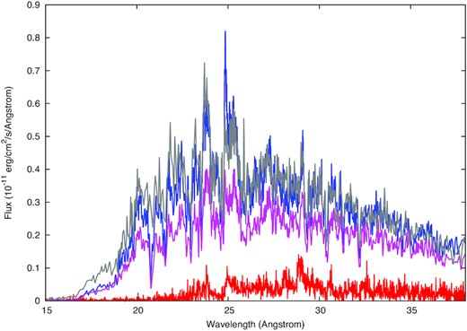
The RGS spectra of Nova LMC 2009 in units of measured flux versus wavelength, observed on days 90 (2009 May, in red), 165 (2009 July, in blue), 197 (2009 August, grey), and 229 (2009 September, purple).
In Fig. 2, we present the EPIC-pn light curves during the four exposures, because the pn is the instrument with the largest count rate and the best time resolution. In all four exposures, there was large aperiodic variability: the count rate varied by an order of magnitude on day 90, by a little more of a factor of 3 on days 165, and by about 60 per cent on days 197 and 229. The MOS and RGS light curves of each exposure are modulated exactly like the pn one. Despite a moderate amount of pileup in the pn spectrum, the irregular variability of the source appeared the same in all instruments. We corrected for pileup by excluding an inner region and leaving only the PSF wing and found that pileup does not affect the proportional amplitude of the irregular variations and light curve trend. Irregular variability over time-scales of hours has been observed at different epochs in the X-ray light curve in several other SSS-novae, most notably in N SMC 2016 (Orio et al. 2018), V1494 Aql (Drake et al. 2003), and in one of the early RS Oph exposures (Nelson et al. 2008). However, RS Oph was observed many times for hours, and we know that the supersoft X-ray flux stabilized in the later exposures. Before proceeding with a spectral analysis, we examined the spectral variability to assess whether it is connected with flux variability.
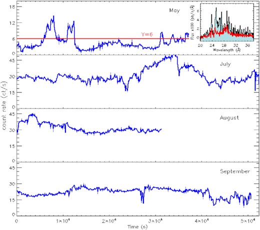
The EPIC-pn light curve, from top to bottom, as measured on days 90, 165, 197, and 229. The red horizontal line in the top panel shows the pn cutoff for the averaged ‘low count rate’ and ‘high count rate’ spectra, shown in the inset in red and black, respectively (note that the RGS count rate varied proportionally to the pn count rate variation).
In the top panel of Fig. 2a, red line indicates the count rate limit of six counts s−1 measured with the pn, chosen for the intervals in which we extracted high and low count rate high-resolution RGS spectra on day 90. This is the only exposure for which we found strong variability in the strength of the spectral features, as shown in the inset in the first panel of the figure. There is especially a striking difference in the 25–28 Å range, where some emission lines were almost present only when the flux increased significantly for short periods. In the other observations (days 165, 197, and 229) the count rate variability was not matched by a change in the spectral shape of the continuum to which most of the flux variation is due. Also, the strength of most emission lines varied less, and the variations mostly followed with the change in the continuum. Fig. 3 shows ‘time maps’, that is variations of each line during the exposures, as well as spectra extracted during two very short intervals of high and low count rates for each observation. We found a correlation of the count rate with the strength of the N vi and N vii lines. The absorption edge of N vii, which abruptly cuts the flux below 18.587 Å, did not vary with the flux level, and for this reason, we rule out that the variability was caused by changes in intrinsic absorption. A likely interpretation of the variability of the continuum flux is that along the line of sight, a partially covering, ‘opaque’ absorber appeared and disappeared. In this scenario, the WD surface is for some time partially obscured by the accretion disc that was not disrupted in the outburst, or by large, optically thick and asymmetric regions of the ejecta. Because of the irregular variability over short time-scales, in Nova LMC 2009, we favour the second hypothesis and elaborate this idea in the Discussion and Conclusions sections. We rule out intrinsic variations of the WD flux, because the nova models indicate that burning occurs at a constant rate; thus, the thin atmosphere above the burning layer can hardly change temperature.
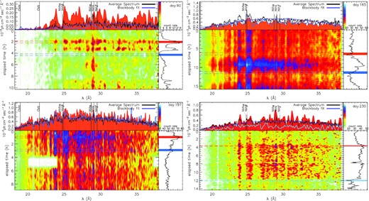
Visualization of the spectral evolution within the observations. The four panels show the fluxed spectra as function of wavelength (top left), colour-coded intensity map as function of time and wavelength (bottom left), and rotated light curve with time on vertical and count rates on horizontal axes (bottom right). In the top right-hand panel, a vertical bar along the flux axis indicates the colours in the bottom left-hand panel. In the top left-hand panel, the red (highest) and blue (lowest) spectra have been extracted during the very short sub-intervals marked in the light curve (bottom right) with shaded areas and bordered by dashed horizontal lines in the bottom left-hand panel. The average spectrum is shown in black, and the dark blue light curve is a blackbody fit obtained assuming depleted oxygen abundance in the intervening medium (see text).
4 IDENTIFYING THE SPECTRAL FEATURES
Identifying the spectral features for this nova appears much more challenging than it has been for other novae observed in the last 15 yr (e.g. Rauch et al. 2010; Ness et al. 2011; Orio et al. 2018, 2020). We started by examining the strongest features. In the spectrum of day 90, we clearly identify two strong emission features: a redshifted Lyman-α H-like line of N vii (rest wavelength 24.78 Å, possibly partially blended with a weaker line of N vi Heβ at 24.889 Å), and the N vi He-like resonance line at 28.78 Å. We fitted the two stronger lines with Gaussian functions and obtained a redshift velocity of 1983 ± 190 km s−1 for the N vii line, and, consistently, a velocity of 1926|$^{+220}_{-250}$| km s−1 for N vi. The integrated flux in these two lines is 1.23 ± 0.18 × 10⁻¹³ erg cm−2 s−1 and 2.37 ± 0.18 × 10⁻¹³ erg cm−2 s−1, respectively.
The spectra of the three following dates, when the SSS was at plateau luminosity, show a forest of features in absorption, and also some in emission. The continua of these spectra appear remarkably similar, but many features varied from one exposure to the next, unlike in other novae observed at the peak of the SSS emission, where the absorption features were not found to change significantly in different exposures done within weeks (e.g. RS Oph, V4374 Sgr, V2491 Cyg, see Nelson et al. 2008; Rauch et al. 2010; Ness et al. 2011). We focused only on the absorption lines that are clearly common to all the last three spectra. In addition to the interstellar absorption lines of O I at 23.51 Å and N I at 31.3 Å, we found only five strong common features, whose profiles we show in Fig. 3. The y-axis shows the averaged RGS1 and RGS2 count rate.
The line of N vii at 24.78 Å appears to have a P-Cyg profile in at least two exposures. Rather than being a ‘true’ P-Cyg, it may be due to the superposition of absorption and emission lines produced in different regions (e.g. absorption in the WD atmosphere, emission farther out in the shell, like in U Sco, see Orio et al. 2013b). The other lines in Fig. 3 are only in absorption. The first three were already observed at almost the same wavelength in other novae (Ness et al. 2011) and were marked as yet ‘unidentified’. We suggest identification of two of these lines as argon: Ar xiii at rest wavelength 29.365 Å, and Ar xiv at 27.631-27.636 Å. We also propose a tentative identification of the Ca XI (30.448 Å) and S xiii (32.239 Å).
Rest wavelength and observed wavelength, velocity, broadening velocity, and optical depth resulting from the fit of spectral lines with proposed identification.
| Ion | λ0 | λm | vshift | vwidth | τc |
|---|---|---|---|---|---|
| (Å) | (Å) | (km s−1) | (km s−1) | ||
| 0610000501 | |||||
| N vii | 24.779 | 24.746 ± 0.005 | −394 ± 66 | 737 ± 154 | 0.0061 ± 0.0034 |
| 24.799 ± 0.049 | +242 ± 94 | ||||
| Ar xiv | 27.636 | 27.615 ± 0.006 | −223 ± 64 | 523 ± 110 | 0.0014 ± 0.0002 |
| Ar xiii | 29.365 | 29.288 ± 0.010 | −789 ± 104 | 1216 ± 202 | 0.0027 ± 0.0003 |
| Ca XI | 30.448 | 30.413 ± 0.008 | −344 ± 75 | 746 ± 117 | 0.0021 ± 0.0003 |
| S xiii | 32.239 | 32.200 ± 0.005 | −361 ± 49 | 539 ± 77 | 0.0023 ± 0.0003 |
| 0604590301 | |||||
| N vii | 24.779 | 24.728 ± 0.006 | −616 ± 67 | 470 ± 106 | 0.0025 ± 0.0004 |
| Ar xiv | 27.636 | 27.599 ± 0.005 | −406 ± 52 | 323 ± 83 | 0.0018 ± 0.0004 |
| Ar xiii | 29.365 | 29.285 ± 0.021 | −813 ± 215 | 1370 ± 596 | 0.0030 ± 0.0013 |
| Ca XI | 30.448 | 30.403 ± 0.006 | −435 ± 63 | 504 ± 95 | 0.0021 ± 0.0003 |
| S xiii | 32.239 | 32.184 ± 0.009 | −513 ± 80 | 630 ± 132 | 0.0022 ± 0.0004 |
| 0604590401 | |||||
| N vii | 24.779 | 24.732 ± 0.006 | −569 ± 71 | 413 ± 119 | 0.0012 ± 0.0004 |
| 24.829 ± 0.004 | +604 ± 54 | ||||
| Ar xiv | 27.636 | 27.621 ± 0.006 | −159 ± 70 | 383 ± 111 | 0.0013 ± 0.0003 |
| Ar xiii | 29.365 | 29.283 ± 0.008 | −835 ± 83 | 1051 ± 149 | 0.0019 ± 0.0002 |
| Ca XI | 30.448 | 30.433 ± 0.006 | −149 ± 57 | 539 ± 87 | 0.0018 ± 0.0002 |
| S xiii | 32.239 | 32.199 ± 0.006 | −370 ± 55 | 767 ± 96 | 0.0021 ± 0.0002 |
The blueshift velocity is modest compared to other novae (RS Oph, see Nelson et al. (2008; V4743 Sgr, see Rauch et al. 2010; and V2491 Cyg, see Ness et al. 2011), N SMC 2016, described in Orio et al. (2018), but this nova was observed as an SSS at a much later post-outburst time. The spread of blueshift velocity was also evident in V2491 Cyg (see Ness et al. 2011).
5 SPECTRAL EVOLUTION AND THE VI ABLE SPECTRAL MODELS
With the gratings, we measure the integrated flux without having to rely on spectral fits like with broad-band data. The flux in the 0.33–1.24 keV (10–38 Å) range increased by only 10 per cent between days 165 and 197, as shown in Table 2. On day 197, the source was also somewhat ‘harder’ and hotter. A decrease by a factor of 1.6 was registered on day 229, when the sources had ‘softened’ again. This evolution is consistent with the maximum temperature estimated with the Swift XRT around day 180 and the following plateau, with final decline of the SSS occurring between days 257 and 279 (Bode et al. 2016). We tried global fits of the spectra, with several steps. Although we did not obtain a complete, statistically significant and comprehensive fit, we were able to test several models and reached a few conclusions in the physical mechanisms from which the spectra originated. We focused mostly on the maximum (day 197), for which we show the result with all all models. The first steps were done by using xspec (Dorman & Arnaud 2001) to fit the models.
Step 1. The first panel of Fig. 4 shows the fit with a blackbody for day 197. We first fitted the spectrum with the TBABS model in xspec (Wilms, Allen & McCray 2000); however, a better fit, albeit not statistically significant yet, was obtained with lower blackbody temperature 47.3 eV (almost 550 000 K), with the TBVARABS formulation by the same authors for the intervening absorbing column N(H). This prescription allows to vary the abundances of the absorbing medium, and in the best fit we could obtain, we varied the oxygen abundance, allowing it to decrease to almost zero, because an absorption edge of O I at 22.8 Å in the ISM makes a significant difference when fitting a smooth continuum like a blackbody. However, it can be seen in Fig. 4 that even the best blackbody fit is not very satisfactory in the hard portion of the spectrum.
Step 2. Assuming, as the models predict (e.g. Yaron et al. 2005; Starrfield et al. 2012; Wolf et al. 2013), and several observations have confirmed (e.g. Ness et al. 2011; Orio et al. 2018) that most of the X-ray flux of the SSS originates in the atmosphere of the post-nova WD, we experimented by fitting atmospheric models for hot WDs burning in shell. We used the grid of TMAP models in Non Local Thermodynamical Equilibrium by Rauch et al. (2010), available in the website: http://astro.uni-tuebingen.de/#rauch/TMAP/TMAP.html. We wanted to evaluate whether the significant X-ray brightening between May and July (day 90 to day 165) was due to the WD shrinking and becoming hotter in the constant bolometric luminosity phase predicted by the nova models (e.g. Starrfield et al. 2012), or to decreasing column density (N(H)) of absorbing material in the shell. In several novae, and most notably in V2491 Cyg (Ness et al. 2011) and N SMC 2016 (Orio et al. 2018), despite blueshifted absorption lines that indicate a residual, fast wind from the photosphere, a static model gives a good first-order fit and predicts most of the absorption features. We moved towards the blue the centre of all absorption lines by a given amount for all lines, leaving the blueshift as a free parameter in the 100–1500 km s−1 range, compatible with the values found in Table 2.
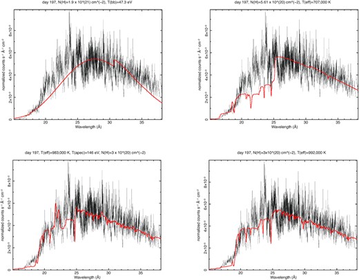
Clockwise, from the top left, comparison of the RGS fluxed spectrum on day 197 with different models, respectively: a blackbody with oxygen-depleted absorbing interstellar medium, a metal-poor model TMAP atmosphere, a metal-rich TMAP atmosphere, and the metal-rich atmosphere with a superimposed thermal plasma component (single temperature) in collisional ionization equilibrium. See Table 3 and text for details.
Table 3 (for all four exposures) and Fig. 4 (for day 197) show the fit with two different grids of models available in the website: http://astro.uni-tuebingen.de/#rauch/TMAP/TMAP.html. In the attempt to optimize the fit, we calculated both the CSTAT parameter (Cash 1979; Kaastra 2017) and the reduced χ2, but we cannot fit the spectrum very well with only the atmospheric model (thus, we do not show the statistical errors in Table 3), since an additional component appears to be superimposed on the WD spectrum and many fine details are due to it. Bode et al. (2016) attributed an unabsorbed luminosity of 3–8 × 1034 erg s−1 to the nova ejecta. Another shortcoming is that the TMAP model does not include argon. Argon L-shell ions are important between 20 and 40 Å and argon may be even enhanced in some novae (the oxygen–neon ones, see José, Hernanz & Iliadis 2006). Above, we have identified indeed two of these argon features that appear strong and quite constant in the different epochs.
Integrated flux measured in the RGS range of 10–38 Å, effective temperature, column density, and unabsorbed flux in the WD continuum resulting from the fit with two atmospheric models with different metallicities, as described in the text: M1 is metal enriched and M2 is metal poor.
| Day | RGS flux | M1 Te | M1 Unabs. flux | M1 N(H) | M2 Te | M2 Unabs. flux | M2 N(H) |
|---|---|---|---|---|---|---|---|
| erg cm−2 s−1 | K | erg cm−2 s−1 | 1020 cm−2 | K | erg cm−2 s−1 | 1020 cm−2 | |
| 90.4 | 5.38 × 10⁻¹² | 738 000 | 1.29 × 10⁻¹¹ | 6.5 | 624 000 | 1.36 × 10⁻¹¹ | 5.7 |
| 164.9 | 8.08 × 10⁻¹¹ | 910 000 | 9.08 × 10⁻¹¹ | 3.5 | 784 000 | 9.08 × 10⁻¹⁰ | 6.1 |
| 196.17 | 1.20 × 10⁻¹⁰ | 992 000 | 9.06 × 10⁻¹¹ | 4.5 | 707 000 | 1.21 × 10⁻¹⁰ | 5.6 |
| 228.93 | 3.91 × 10⁻¹¹ | 947 000 | 5.89 × 10⁻¹¹ | 3.0 | 701 000 | 7.29 × 10⁻¹¹ | 4.4 |
Model 1 (M1) is model S3 of the ‘metal-rich’ grid (used by Bode et al. (2016) for the broad-band Swift spectra), including all elements up to nickel, and Model 2 (M2) is from the metal-poor ‘halo’ composition grid, studied for non-nova SSS sources in the halo or Magellanic Clouds, which are assumed to have accreted metal-poor material and may have undergone only very little mixing above the burning layer. The nitrogen and oxygen mass abundance in model S3 are as follows: nitrogen is 64 times the solar value and oxygen is 34 times the solar value. In contrast, carbon is depleted because of the CNO cycle and is only 3 per cent the solar value.
Novae in the Magellanic Clouds may not be similar to the non-ejecting SSS. They may be metal-rich and not have retained the composition of the accreted material, since convective mixing is fundamental in causing the explosion, heating the envelope, and bringing towards the surface β+ decaying nuclei (Prialnik 1986). The first interesting fact is that adopting the TBVARABS formulation like for a blackbody does not make a significant difference in obtaining the best fit. In fact, the atmospheric models have strong absorption edges and features that ‘peg’ the model at a certain temperature and are much more important in the fit than any variation in the N(H) formulation, especially with low-absorbing column like we have towards the LMC. In the following context, we show models obtained only with TBABS (fixed solar abundances).
Both the metal-poor and metal-enriched models imply a very compact and massive WD, with logarithm of the effective gravity log(g) = 9. In fact, the resulting effective temperature is too high for a less compact configuration and the SSS would have largely super-Eddington luminosity. Table 4 does not include the blueshift velocity, which was a variable parameter but was fixed for all lines: it is in the 300–600 km s−1 for each best fit, consistently with the measurements in Table 2.
Main parameters of the best fits obtained by adding three BVAPEC components to the enhanced abundances TMAP model and allowing the nitrogen abundance to vary. The flux is the unabsorbed one. The N(H) minimum value of 3 × 1020 cm−2 and the fit converged to the minimum value in the second and fourth observations. We also assumed a minimum BVAPEC temperature of 50 eV.
| Parameter | Day 90.4 ‘high spectrum’ | Day 164.9 | Day 196.17 | Day 228.93 |
|---|---|---|---|---|
| N(H) × 1020 (cm−2) | 8.7|$^{+3.8}_{-1.8}$| | 3 | 6.8|$_{-1.9}^{+4.2}$| | 3 |
| Teff (K) | 736 000|$^{+11,000}_{-21,000}$| | 915 000 ± 5000 | 978 000 ± 5000 | 907 000 ± 5000 |
| FSSS,un × 10−11 (erg s−1 cm−2) | 2.64|$_{-0.71}^{+1.52}$| | 7.69|$_{-0.04}^{+0.01}$| | 9.49|$_{-0.17}^{+0.20}$| | 5.58|$_{-0.08}^{+0.16}$| |
| kT1 (eV) | 50|$^{+8}_{-0}$| | 55|$_{-5}^{+2}$| | 68 ± 8 | 55|$_{-9}^{+2}$| |
| Fun,1 × 10−11 (erg s−1 cm−2) | 0.71|$_{-0.69}^{+0.70}$| | 0.12|$_{-0.02}^{+0.05}$| | 5.83|$_{-2.50}^{+11.00}$| | 0.17|$_{-0.16}^{+0.26}$| |
| kT2 (eV) | 114|$_{-18}^{+22}$| | 134 ± 2 | 152 ± 6 | 127 ± 8 |
| Fun,2 × 10−12 (erg s−1 cm−2) | 1.74|$^{+1.00}_{-0.70}$| | 3.29 ± 0.03 | 4.45|$^{+6.00}_{-4.00}$| | 1.93|$_{-0.29}^{+0.46}$| |
| kT3 (eV) | 267|$_{-165}^{+288}$| | 176 ± 3 | 174 ± 10 | 177 ± 6 |
| Fun,3 × 10−12 (erg s−1 cm−2) | 0.77|$^{+1.00}_{+17.57}$| | 5.56 ± 0.50 | 4.46|$_{-4.00}^{+5.21}$| | 3.29 ± 0.39 |
| Fun,total × 10−11 (erg s−1 cm−2) | 3.60 | 8.69 | 16.21 | 6.28 |
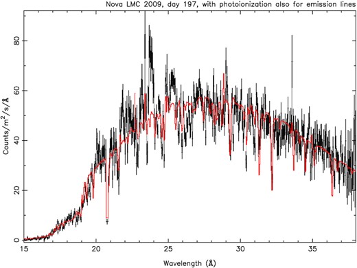
In Fig. 4, we show the atmospheric fits for day 197. The metal-rich model, with higher effective temperature, appears more suitable. We note that in the last three spectra, whose best-fitting parameters are shown in Table 3, the value of the column density N(H) for this model was limited to a minimum value of 3 × 1020 cm−2, consistently with LMC membership. The fact that the metal-rich model fits the spectrum better indicates that, even in the low-metallicity environment of the LMC, the material in the nova outer atmospheric layers during a mass-ejecting outburst mixes up with ashes of the burning and with WD core material. The WD atmosphere is thus expected to be metal-rich and especially rich in nitrogen. However, the metal-rich model overpredicts an absorption edge of N vii at 18.587 Å, which is instead underpredicted by the ‘halo’ model. This is a likely indication that the abundances may be a little lower than in Galactic novae, for which the ‘enhanced’ TMAP better fits the absorption edges (e.g. Rauch et al. 2010). The metal-rich model indicates that the continuum is consistent with a WD at effective temperature around 740 000 ± 50 000 K on day 90, and hotter in the following exposures, reaching almost a million K on day 197. Although the fit indicates a decrease in intrinsic absorption after the first observation, the increase in apparent luminosity is mostly due to the increase in effective temperature, and we conclude that the WD radius was contracting until at least day 197.
The ‘enriched’ model atmosphere seems to be the most suitable in order to trace the continuum, except for the excess flux above 19 Å. Because the continuum shape of the atmospheric model does not change with the temperature smoothly or ‘incrementally’ like a blackbody, and is extremely dependent on the absorption edges, we cannot obtain a better fit by assuming an absorbing medium depleted of oxygen (or other element). This is the same also for the ‘halo’ model. Therefore, the fits we show were obtained all only with TBABS, assuming solar abundances in the intervening column density between us and the source.
Step 3. In these spectra, we do not detect He-like triplet lines sufficiently well in order to use line ratios as diagnostics (see, for instance, Orio et al. 2020, and references therein). In the last panel in Fig. 4, we show the fit with TMAP and a component of thermal plasma in collisional ionization equilibrium (BVAPEC in xspec, see Smith et al. 2001). The fit improvement is an indication that many emission lines from the nova outflow are superimposed on the SSS emission, but clearly a single thermal component is not sufficient to fit the whole spectrum. Nova shells may have luminous emission lines in the supersoft range after a few months from the peak of the outburst (V382 Vel, V1494 Aql Ness et al. 2005; Rohrbach, Ness & Starrfield 2009). Such emission lines in the high-resolution X-ray spectra of novae are still measured when the SSS is eclipsed or obscured (Ness et al. 2013), indicating an origin far from the central source. Shocked ejected plasma in collisional ionization equilibrium has been found to originate the X-ray emission of several novae, producing emission features in different ranges, from the ‘hard’ spectrum of V959 Mon (Peretz et al. 2016) to the much ‘softer’ spectrum of T Pyx (Tofflemire et al. 2013).
Adding only one such additional component with plasma temperature keV improves the fit by modelling oxygen emission lines, but it does not explain all the spectrum in a rigorous way. The fit improved by adding one more BVAPEC component, and improved incrementally, when a third one was added. The fits shown in Fig. 4 yield a reduced χ2 parameter still of about 3, due to many features that are are still unexplained. Also, the N vii K-edge remains too strong and this is not due to an overestimate of N(H), since the soft portion of the flux is well modelled. In Fig. 5 and in Table 4, we show fits with three BVAPEC components of shocked plasma in collisional ionization equilibrium. To limit the number of free parameters, the results we present in Table 4 were obtained with variable nitrogen abundances as free parameter, which turned out to reach even values around ≃500 for one of the components. We obtain a better fit if the nitrogen abundance is different in the three components, but different ‘combinations’ of temperature and nitrogen abundance give the same goodness of the fit. We also tried fits leaving free also the oxygen and carbon abundances, leaving the other abundances at solar values: although the fit always converged with al least one of these elements enhanced in at least one plasma component, there was no clear further improvement. The best composite fit with ‘free’ nitrogen is shown in Fig. 5 for all four spectra. Some emission lines are still unexplained, indicating a complex origin, probably in many more regions of different temperatures and densities. The fits are not statistically acceptable yet, with a reduced value of χ2 of 1.7 for the first spectrum, about 3 for the second and third, and 4.7 for the fourth (we note that adopting cash statistics did not result in very different or clearly improved fits); however, the figure shows that the continuum is well modelled and many of the emission lines are also explained.

Step 4. Since we could not model all the emission lines with the collisional ionization code, the next step was to explore a photoionization code. We used the PION model (Mehdipour, Kaastra & Kallman 2016) in the spectral fitting package SPEX (Kaastra, Mewe & Nieuwenhuijzen 1996), having also a second important aim: exploring how the abundances may change the continuum and absorption spectrum of the central source. In fact, SPEX allows to use PION also for the absorption spectrum. The photoionizing source is assumed to be a blackbody, but the resulting continuum is different from that of a simple blackbody model, because the absorbing layers above it remove emission at the short wavelengths, especially with ionization edges (like in the static atmosphere). An important difference between PION and the other photoionized plasma model in SPEX, XABS, previously used for nova V2491 Cyg (Pinto et al. 2012), is that the photoionization equilibrium is calculated self-consistently using available plasma routines of SPEX (in XABS instead, the photoionization equilibrium was pre-calculated with an external code). The atmospheric codes like TMAP include the detailed microphysics of an atmosphere in non-local thermodynamic equilibrium, with the detailed radiative transport processes, that are not calculated in PION; however, with PION, we were able to observe how the line profile varies with the wind velocity and, most important, to vary the abundances of the absorbing material. This step is thus an important experiment, whose results may be used to calculate new, ad hoc atmospheric calculations in the future. The two most important elements to vary in this case are nitrogen (enhanced with respect to carbon and to its solar value because of mixing with the ashes in the burning layer) and oxygen (also usually enhanced with respect to the solar value in novae). We limited the nitrogen abundance to a value of 100 times the solar value and found that this maximum value is the most suitable to explain several spectral features. Oxygen in this model fit is less enhanced than in all TMAP models with ‘enhanced’ abundances, resulting to be 13 times the solar value. With such abundances, and with depleted oxygen abundances in the intervening ISM (the column density of the blackbody), we were able to reproduce the absorption edge of nitrogen and to fit the continuum well. It is remarkable that this simple photoionization model, with the possibility of ad hoc abundances as parameters, fits the continuum and many absorption lines better than the TMAP atmospheric model.
To model some of the emission lines, we had to include a second PION component, suggesting that the emission spectrum does not originate in the same region as the absorption one, as we suggested above. Table 5 and Fig. 6 show the best fit obtained for day 197. Due to the better continuum fit, even if we seem to have modelled fewer emission lines, χ2 here was about 2 (compared to a value of 3 in Fig. 5). The blackbody temperature of the ionizing source is 70 keV, or about 812 000 K, and its luminosity turns out to be Lbol = 7.03 × 1037 erg s−1, and by making the blackbody assumption, we know that these are only lower and upper limits, respectively, for the effective temperature and bolometric luminosity of the central source (see discussion by Heise, van Teeseling & Kahabka 1994). The X-ray luminosity of the ejecta is 1036 erg s−1, or 1.5 per cent of the total luminosity.
Fit to the spectrum of day 197 with two PION regions as in Table 5.
Main physical parameters of the SPEX Black Body(BB)+2-PION model fit for day 197. ISM indicates values for the intervening interstellar medium column density. The errors (67% confidence level) were calculated only for the PION in absorption, assuming fixed parameters for PION in emission. The abundance values marked with (*) are parameters that reached the lower and upper limits.
| N(H)ISM | 9.6 ± 0.4 × 1020 cm−2 |
| 0/0⊙ (ISM) | 0.06 (*) |
| TBB | 812,000 ± 3020 K |
| RBB | 8 × 108 cm |
| LBB | 7 ± 0.2 × 1037 erg s−1 |
| N(H)1 | 6.4|$^{+2.5}_{-1.9} \times 10^{21}$| cm−2 |
| vwidth (1) | 161 ± 4 km s−1 |
| vblueshift (1) | 327|$^{+16}_{-21}$| km s−1 |
| N/N⊙ | 100−7 (*) |
| 0/0⊙ | 13 ± 2 |
| ξ (1) | 489.7|$^{+50}_{-30}$| erg cm |
| |$\dot{m}$| | 1.84 × 10⁻⁸ M⊙ yr−1 |
| ne (1) | 2.85 × 108 cm−3 |
| N(H)2 | 2.6 × 1019 cm−2 |
| vwidth (2) | 520 km s−1 |
| vredshift (2) | 84 km s−1 |
| ξ (2) | 30.2 erg cm |
| ne (2) | 2.87 × 104 cm−3 |
| LX (2) | 1.1 × 1036 erg s−1 |
An interesting fact is that we were indeed able to explain several emission features but not all. It is thus likely that there is a superposition of photoionization by the central source and ionization due to shocks in colliding winds in the ejecta. However, we did not try any further composite fit, because too many components were needed and we found that the number of free parameters is too large for a rigorous fit. In addition, the variability of some emission features within hours make a precise fit an almost impossible task.
Assuming LMC distance of about 49.6 kpc (Pietrzyński et al. 2019), the unabsorbed flux in the atmospheric models at LMC distance implies only X-ray luminosity close to 4 × 1036 erg s−1 on the first date, peaking close to ≃2.7 × 1037 erg s−1 on day 197 (although the model for that date includes a ≃60 per cent addition to the X-ray luminosity due to a very bright plasma component at low temperature, 70 eV, close to the the value obtained with PION for the blackbody-like ionizing source). We note that the X-ray luminosity with the high Teff we observed represents over 98 per cent of the bolometric luminosity of the WD. Thus, the values obtained with the fits are a few times lower than the post-nova WD bolometric luminosity exceeding 1038 erg s−1 , predicted by the models (e.g. Yaron et al. 2005). Even if the luminosity may be higher in an expanding atmosphere (van Rossum 2012), it will not exceed the blackbody luminosity of the PION fit, 7 × 1037 erg s−1, which is still a factor of 2–3 lower than Eddington level. Although several novae have become as luminous SSS as predicted by the models (see N SMC 2016, Orio et al. 2018), in other post-novae, much lower SSS luminosity has been measured, and in several cases, this has been attributed to an undisrupted, high inclination accretion disc acting as a partially covering absorber (Ness et al. 2015), although also the ejecta can cause this phenomenon, being opaque to the soft X-rays while having a low filling factor. In U Sco instead, the interpretation for the low observed and inferred flux was different. It is in fact very likely that only observed Thomson-scattered radiation was observed, while the central source was always obscured by the disc (Ness et al. 2012; Orio et al. 2013b). However, also the reflected radiation of this nova was thought to be partially obscured by large clumps in the ejecta in at least one observation (Ness et al. 2012).
In the X-ray evolution of N LMC 2009, one intriguing fact is that not only the X-ray flux continuum but also that the emission features clearly increased in strength after day 90. This seems to imply that these features are either associated with or originate very close to the WD to which we attribute the SSS continuum flux.
Step 5. An additional experiment we did with spectral fitting was with the ‘expanding atmosphere’ ‘wind-type’ WT model of van Rossum (2012), which predicts shallower absorption edges and may explain some emission features with the emission wing of atmospheric P-Cyg profiles. One of the parameters is the wind velocity at infinite, which does not translate in the observed blueshift velocity. The P-Cyg profiles become ‘smeared out’ and smoother as the wind velocity and the mass loss rate increase. Examples of the comparison of the best model with the observed spectra, plotted with IDL and obtained by imposing the condition that the flux is emitted from the whole WD surface at 50 kpc distance, are shown for days 90 and 197 in Fig. 7 in the top panel. The models shown are those in the calculated grid that best match the spectral continuum; however, there are major differences between model and observations. Next, we assumed that only a quarter of the WD surface is observed, thus choosing models at lower luminosity, but we obtained only a marginally better match. The interesting facts are: the mass outflow rate is about the same as estimated with SPEX and the PION model, (b) this model predicts a lower effective temperature for the same luminosity, and (c) most emission features do not seem to be possibly associated with the ‘wind atmosphere’ as calculated in the model. It is not unrealistic to assume that they are produced farther out in the ejected nebula, an implicit assumption in the composite model of Table 4 and Fig. 5.
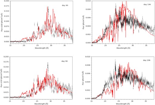
Comparison of the ‘WT model’ with the observed spectra on day 90 (averaged spectrum) and day 197. In the upper panels, the condition that the luminosity matched that observed at 50 kpc is imposed, assuming for days 90 and 197, respectively: Teff = 500 000 K, log(geff) = 7.83, N(H) = 2 × 1021 cm−2, |$\dot{m} = 2 \times 10^{-8}$| M⊙ yr−1, v∞ = 4800 km s−1 and Teff-550 000 K, log(geff) = 8.30, |$\dot{m} = 10^{-7}$| M⊙ yr−1, N(H) = 1.5 × 1021 cm−2, and v∞ = 2400 km s−1. In the lower panels, the assumption was made that only a quarter of the WD surface is observed, and the parameters are Teff = 550 000 K, log(geff) = 8.08, |$\dot{m} = 10^{-8}$| M⊙ yr−1, N(H) = 1.8 × 1021 cm−2 v∞ = 2400 km s−1 and Teff-650 000 K, log(geff) = 8.90, |$\dot{m} = 2 \times 10^{-8}$| M⊙ yr−1, N(H) = 2 × 1021 cm−2, and v∞ = 4800 km s−1, respectively, for days 90 and 197.
6 COMPARISON WITH THE SPECTRA OF OTHER NOVAE
To date, 25 novae and SSSs have been observed with X-ray gratings, often multiple times, so a comparison with other novae in the supersoft X-ray phase is useful and can be correlated with other nova parameters. While the last part of this paper illustrates an archival search in X-ray data of other MC novae, in this section, we analyse some high-resolution data of Galactic and Magellanic Clouds (MC) novae bearing some similarity with N LMC 2009.
(1) Comparison with U Sco. The first spectrum (day 90) can be compared with one of U Sco, another RN that has approximately the same orbital period (Orio et al. 2013b). In this section, all the figures illustrate the fluxed spectra. In U Sco, the SSS emerged much sooner and the turn-off time was much more rapid. Generally, the turn-off and turn-on time are both inversely proportional to the mass of the accreted envelope, and Bode et al. (2016) note that this short time is consistent with the models’ predictions for a WD mass 1.1<m(WD)<1.3 M⊙, which is also consistent with the high effective temperature. However, the models by Yaron et al. (2005), who explored a large range of parameters, predict only relatively low ejection velocities for all RN and there is no set of parameters that fits a very fast RN like U Sco, with large ejection velocity and short decay times in optical and X-rays. Thus, the specific characteristics of U Sco may be due to irregularly varying |$\dot{m}$| and/or other peculiar conditions that are not examined in the work by Yaron et al. (2005). The parameters of N LMC 2009, instead, compared with Yaron et al. (2005), are at least marginally consistent with their model of a very massive (1.4 M⊙), initially hot WD (probably recently formed).
Fig. 8 shows the comparison of the early Chandra spectrum (day 18) of U Sco (Orio et al. 2013b), with the first spectrum (day 90) of N LMC2009. The apparent P-Cyg profile of the N vii H-like line with rest wavelength 24.78 Å and the N vi He-like resonance line with rest wavelength 28.78 Å is observed in N LMC 2009 like in U Sco, with about the same redshift for the emission lines and lower blueshift for the absorption. The definition ‘pseudo P-Cyg’ in Orio et al. (2013b) was adopted, because there is clear evidence that the absorption features of U Sco in the first epoch of observation were in the Thomson-scattered radiation originally emitted near or on the WD surface. The emission lines originated in an outer region in the ejecta at large distance from the WD.
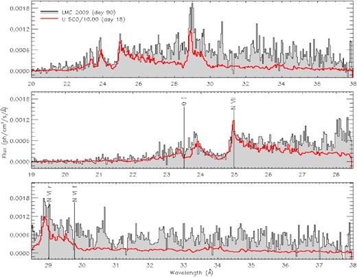
The XMM–Newton RGS X-ray spectrum of Nova LMC 2009a on day 90 of the outburst (grey), compared in the left-hand panel with the Chandra Low Energy Transmission Gratings of U Sco on day 18, with the photon flux multiplied by a factor of 10 for N LMC 2009a (red). The distance to U Sco is at least 10 kpc (Schaefer et al. 2010) or 5 times larger than to the LMC, so the absolute X-ray luminosity of N LMC 2009a at this stage was about 2.5 times that of U Sco. H-like and He-like resonance and forbidden line of nitrogen are marked, with a redshift 0.008 (corresponding to 2400 km s−1, measured for the U Sco emission features). These features in U Sco were also measured in absorption with a blueshift corresponding to 2000 km s−1, producing an apparent P-Cyg profile. We also indicate the O I interstellar absorption at rest wavelength.
Apart from the similarity in the two strong nitrogen features, the spectrum of N LMC 2009 at day 90 is much more intricate than that of U Sco and presents a ‘forest’ of absorption and emission features that are not easily disentangled, also given the relatively poor S/N ratio. U Sco, unlike N LMC 2009a, never became much more X-ray luminous (Orio et al. 2013b) and the following evolution was completely different from that of N LMC 2009, with strong emission lines and no more measurable absorption features. Only a portion of the predicted WD flux was detected in U Sco, and assuming a 12-kpc distance for U Sco (Schaefer et al. 2010), N LMC 2009a was twice intrinsically more luminous already at day 90, ahead of the X-ray peak, although above 26 Å the lower flux of U Sco is due in large part to the much higher interstellar column density (Schaefer et al. 2010; Orio et al. 2013b), also apparent from the depth of the O I interstellar line. U Sco did not become more luminous in the following monitoring with the Swift XRT (Pagnotta et al. 2015). Given the following increase in the N LMC 2009 SSS flux, we suggest that in this nova, we did not observe the supersoft flux only in a Thomson-scattered corona in a high inclination system, like in U Sco, but probably there was a direct view of at least a large portion of the WD surface.
(2) Comparison with KT Eri. A second comparison, shown in Fig. 9 and more relevant for the observations from day 165, is with unpublished archival observations of KT Eri, a Galactic nova with many aspects in common with N LMC 2009a, including the very short-period modulation in X-rays (35 s, see Beardmore et al. 2010; Ness et al. 2015). Fig. 9 shows the spectrum of N LMC 2009 on day 165 overimposed on the KT Eri spectrum observed with Chandra and the Low Energy Transmission Grating (LETG) on day 158 (Ness et al. 2010; Orio et al. 2018).
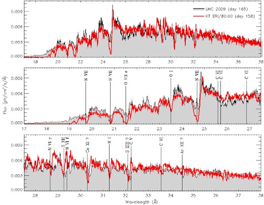
Comparison of the spectrum of N LMC 2009 on day 165 with the spectrum of KT Eri on day 158, with the photon flux of N LMC 2009 divided by a factor of 80. In the panel on the left, we indicate the line’s position with a blueshift by 1410 km s−1, which is a good fit for several absorption lines of KT Eri predicted by the atmospheric models (except for O I and N I, which are local ISM lines, observed at rest wavelength).
The KT Eri GAIA parallax in DR2 does not have a large error and translates into a distance of 3.69|$^{+0.53}_{-0.33}$| kpc.1 The total integrated absorbed flux in the RGS band was 10−8 erg s−1 cm−2, and the absorption was low, comparable to that of the LMC (Pei et al. 2021) implying that N LMC 2009 was about 2.3 times more X-ray luminous than KT Eri, although this difference may be due to the daily variability observed in both novae. Bode et al. (2016) highlighted, among other similarities, a similar X-ray light curve. However, there are some significant differences in the Swift XRT data: the rise to maximum supersoft X-ray luminosity was only about 60 d for KT Eri, and the decay started around day 180 from the outburst, shortly after the spectrum we show here. The theory predicts that the rise of the SSS is inversely proportional to the ejecta mass. The duration of the SSS is also a function of the ejected mass, which tends to be inversely proportional to both the WD mass and the mass accretion rate before the outburst (e.g. Wolf et al. 2013). The values of Teff for N LMC 2009a indicate a high-mass WD and the time for accreting the envelope cannot have been long, with a low-mass accretion rate, since it is an RN. The other factor contributing to accreting higher envelope mass is the WD effective temperature at the first onset of accretion (Yaron et al. 2005). This would mean that the onset of accretion was recent in N LMC 2009a and its WD had a longer time to cool than KT Eri before accretion started.
KT Eri was observed earlier after the outburst with Chandra and the LETG, showing a much less luminous source on day 71 after the outburst, then a clear increase in luminosity on days 79 and following dates. The LETG spectrum of KT Eri appeared dominated by a WD continuum with strong absorption lines from the beginning, and in no observation did it resemble that of N LMC 2009a on day 90. Unfortunately, because of technical and visibility constraints, the KT Eri observations ended at an earlier post-outburst phase than the N LMC 2009a ones. However, some comparisons are possible. Fig. 9 shows the comparison between the KT Eri spectrum of day 158 and the N LMC 2009 spectrum of day 165. We did not observe flux shortwards of an absorption edge of O vii at 18.6718 Å for KT Eri, but there is residual flux above this edge for N LMC 2009a, probably indicating a hotter source. We indicate the features assuming a blueshift velocity of 1400 km s−1, more appropriate for KT Eri, while the N LMC 2009 blueshift velocity is on average quite lower. The figure also evidentiates that in N LMC 2009, there may be an emission core superimposed on blueshifted absorption for the O vii triplet recombination He-like line with rest wavelength 21.6 Å.
N LMC 2009 does not share with KT Eri, or with other novae (see Rauch et al. 2010; Orio et al. 2018) a very deep absorption feature of N viii at 24.78 Å, which was almost saturated in KT Eri on days 78–84. It appears like a P Cyg profile as shown in Fig. 10, and the absorption has lower velocity of few hundred km s−1. Despite many similarities in the two spectra, altogether the difference in the absorption lines depth is remarkable. The effective temperature upper limit derived by Pei et al. (2021 preprint, private communication) for KT Eri is 800 000 K, but the difference between the two novae is so large that it seems to be not only due to a hotter atmosphere (implying a higher ionization parameter): we suggest that abundances and/or density must also be playing a role.
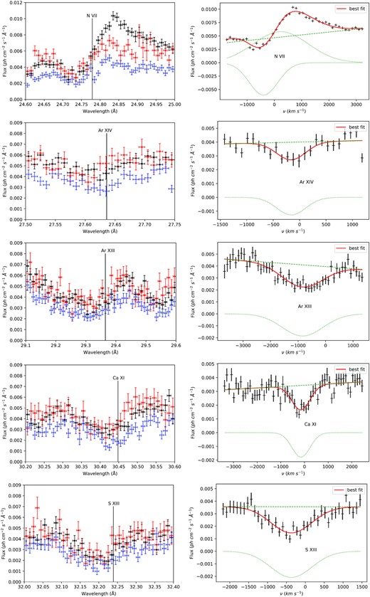
On the left, the profiles of common features observed with the RGS (averaged RGS1 and RGS2) at days 165 (red), 197 (black), and 229 (blue). On the right, in velocity space, the same line and the fit for day 229 (N vii) and for day 197 (other plots).
(3) Comparison with Nova SMC 2016. In Fig. 11, we show the comparison of the N LMC 2009 day 197 spectrum with the last high-resolution X-ray spectrum, obtained on day 88, for N SMC 2016 (Aydi et al. 2018a; Orio et al. 2018). The evolution of N SMC 2016 was much more rapid, the measured supersoft X-ray flux was larger by more than an order of magnitude, and the unabsorbed absolute luminosity was larger by a factor of almost 30 (see Table 2, and Orio et al. 2018). The lines of N vii (rest wavelength 24.78 Å), N vi recombination (28.79 Å), and C vi (33.7342 Å) seem to be in emission for N LMC 2009a, but they are instead observed in absorption for N SMC 2016. The absorption features of N SMC 2016 are also significantly more blueshifted by about 2000 km s−1 in N SMC 2016. The effective temperature in this nova was estimated by Orio et al. (2018) as 900 000 K in the spectrum shown in the figure. The comparison shows that N LMC 2009 was probably hotter and/or had a denser photoionized plasma.
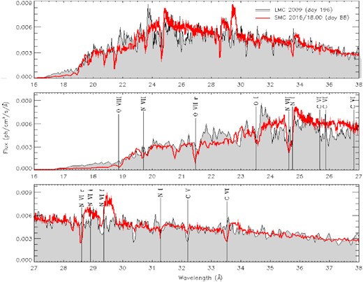
Comparison of the spectrum of N LMC 2009 on day 165 with the spectrum of N SMC 2016 on day 88, with the photon flux of N LMC 2009 multiplied by a factor of 18 for the comparison.
(4) Finally, another significant comparison can be made with N LMC 2012 (for which only one exposure was obtained , see Schwarz et al. 2015), the only other MC nova for which an X-ray high resolution spectrum is available. Despite the comparable count rate, the spectrum of N LMC 2012 shown by Schwarz et al. (2015) is completely different from those of N LMC 2009. It has a much harder portion of high continuum, which is not present in other novae, and the flux appears to be cut only by the O viii absorption edge at 14.228 Å. We note here that only the continuum X-ray spectrum in this nova appears to span a much larger range than in most other novae, including N LMC 2009a. We did attempt a preliminary fit with WD atmospheric models for this nova and suggest the possible presence in the spectrum of two separate zones at different temperature, possibly due to magnetic accretion on to polar caps, like suggested to explain the spectrum of V407 Lup (Aydi et al. 2018b).
7 TIMING ANALYSIS: REVISITING THE 33-s PERIOD
Ness et al. (2015) performed a basic timing analysis for the XMM–Newton observations, detecting a significant modulation with a period around 33.3 s. The period may have changed by a small amount between the dates of the observations. Here, we explore this modulation more in detail, also with the aid of light curves’ simulations. Such short period modulations have been detected in other novae (see Ness et al. 2015; Page et al. 2020) and non-nova SSS (Trudolyubov & Priedhorsky 2008; Odendaal et al. 2014). Ness et al. (2015) attributed the modulations to non-radial g-mode oscillations caused by the burning that induces gravity waves in the envelope (so called ϵ mechanism, but recently, detailed models seem to rule it out because the typical periods would not exceed 10 s (Wolf, Townsend & Bildsten 2018). Other mechanisms invoked to explain the root cause of the pulsations are connected with the WD rotation. If the WD accretes mass at high rate, the WD may be spun to high rotation periods. In CAL 83, the oscillations have been attributed by Odendaal & Meintjes (2017) to ‘dwarf nova oscillations’ in an extreme ‘low-inertia magnetic accretor’.
7.1 Periodograms
We compared periodograms of different instruments and exposures. Because the low count rate of the RGS resulted in low-quality periodograms or absent signal, we focused on the EPIC cameras, despite some pileup, which effects especially the pn.
In Fig. 12, we show and compare all the calculated periodograms. Even though the reading times were uniform, we used the Lomb–Scargle (Scargle 1982) method, because it allows to better resolve the period than the Fourier transform, due to oversampling. We show a larger time interval in the left insets, while the most important features are shown in the main panels. Table 6 summarizes the most significant periodicities with errors estimated from the half width at half-maximum of the corresponding peaks. The periodograms for the light curves measured on days 90 and 229 do not show an obviously dominant signal in the other observations (although, as Table 3 shows, we retrieved the period in the pn light curve on day 229, with lower significance), so we did not investigate these data further. It is very likely that the modulation started only in the plateau phase of the SSS and ceased around the time the final cooling started. For the data of days 165 and 197, we found dominant peaks, especially strong on day 197. The dominant signal is absent in the MOS light curve of day 165 but was retrieved instead in the RGS data of the same date. Both periodograms suggest a single signal, with a double structure in the pn, which, however, may be an artefact. Moreover, the periodicity measured with the RGS data on day 165 is the average of the two values measured with the pn on the same day. This may indicate that the amplitude in the pn light curve is not stable, generating a false beat like in V4743 Sgr (Dobrotka & Ness 2017). The beat causes us to measure a splitting of the peak, while the real signal is in between (so, it may be P4 detected in the RGS data).
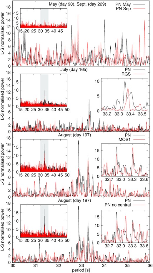
Comparison of periodograms of different instruments and observations. The pileup corrected pn data (pn no central) were extracted after subtracting the central, most piled up region of the source. The insets on the left show larger period intervals, and the shaded areas are the intervals plotted in the main panels. The insets on the right show instead a narrower period interval than the main panels, with the 2009 August periodogram plotted in red.
Detected periodicities, in seconds, corresponding to the strongest signals shown in Fig. 12. We include a possible periodicity in the September data of day 229, although the corresponding peak is not by any means as dominant as on days 165 and 197. In each row, we report periods that are consistent with each other within the statistical error.
| Label | pn | RGS | pn | pn no-pileup | MOS1 | pn |
|---|---|---|---|---|---|---|
| Day 164.9 | Day 164.9 | Day 196.17 | Day 196.17 | Day 196.17 | Day 228.93 | |
| P1 | – | – | 32.89 ± 0.02 | 32.90 ± 0.02 | 32.89 ± 0.02 | 32.89 ± 0.01 |
| P2 | – | – | – | 33.13 ± 0.02 | – | – |
| P3 | 33.35 ± 0.02 | – | 33.31 ± 0.02 | 33.32 ± 0.02 | 33.31 ± 0.02 | – |
| P4 | – | 33.38 ± 0.01 | – | – | – | – |
| P5 | 33.41 ± 0.01 | – | – | – | – | – |
The pattern is more complex on day 197. The periodicity P3 detected in July is retrieved in all the August light curves, suggesting that this feature is real and stable. Moreover, the non-pileup-corrected and the pileup-corrected pn periodograms, and the MOS-1 periodograms, for day 197 show the same patterns, implying that pileup in the pn data does not strongly affect the timing results. We were interested in exploring whether the non-pileup-corrected light curves, which have higher S/N, also give reliable results. For the day 197 observation, we compared the results using the pileup-corrected pn light curve to those obtained for the MOS-1 and found that the derived periodicities (P1 and P3) agree within the errors. Worth noting is the dominant peak P2 in the non-pileup-corrected pn data, measured also in the pileup-corrected light curve, but with rather low significance. We note that also many of the low peaks and faint features are present in both periodograms but with different power. This confirms that pileup does not affect the signal detection, although we cannot rule out that it affects its significance.
7.2 Is the period variable?
The complex pattern discovered in the light curve of day 197 suggests that the period may have varied during the exposure. We already mentioned the variable amplitude on day 165 and reminded that variable amplitude was discovered in the case of V4743 Sgr (Dobrotka & Ness 2017). In Appendix 1, we show how we used simulations to investigate the possibility of variable periodicity and amplitude. The conclusion that can be derived is that models with variable periodicity match the data better than those with a constant period. The lingering question is whether different periodicities occur simultaneously, or whether instead the period of the modulation changes on short time-scales, in the course of each exposure. We reasoned that if the period varied during the exposures, this must become evident by splitting the original exposure in shorter intervals. Therefore, we experimented by dividing the day 197 light curve into two and three equally long segments. The corresponding periodograms are depicted in Fig. 13. Dividing the light curve into halves shows that the first half comprises both dominant signals P1 and P3, while the second half is dominated only by P3. We tried a further subdivision in three parts and found that the first interval is dominated by P1, the second by P2 and P3 (with a slight offset), and in the third portion, none of the P1, P2, and P3 periods can be retrieved. This indicates that the period of the modulation was most likely variable during the exposure. This is probably the reason for which different periods of similar length were measured in the same periodogram by analysing the light curve of the whole exposure time. We suggest that these periods did not coexist but instead, a single modulation occurred, whose amplitude slightly changed during time intervals of minutes to hours. While Ness et al. (2015) found that the short-term periodicity may be a recurrent and transient phenomenon, here instead our interpretation is that the variations in amplitude and length of the period sometimes make it undetectable, but most likely it is always present.
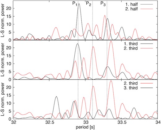
Periodograms for day 197, divided into halves and thirds. The vertical dashed lines indicate the periods P1, P2, and P3 obtained by analysing the whole exposure at once.
8 DISCUSSION: N LMC 2009 A
Nova LMC 2009 is only one of three novae in the Clouds that could be observed with high-resolution X-ray spectroscopy. The others were N LMC 2012 (Schwarz et al. 2015) and N SMC 2016 (Orio et al. 2018). All three novae are luminous and reached a range of effective temperature that can be explained only with the presence of a massive WD, close to the Chandrasekhar limit if we compare the data with models by Yaron et al. (2005). However, a word of warning should be given concerning the fact the models do not explain all the RN characteristics in a very consistent way. In fact, the ejection velocity inferred from the optical spectra exceeds the value predicted by the models for an RN with a recurrence period of 38 yr or shorter: this difficulty of modelling RN is a known problem. A possible explanation is that |$\dot{m}$| has been variable over the secular evolution of these novae: if the recurrence time was longer, and |$\dot{m}$| was lower in previous epochs, the closely spaced nova outbursts have started only very recently and the material in the burning layer may still be colder and more degenerate than it would be after many outbursts with a very short recurrence time, thus causing a larger ejection velocity than in the models, which assume that the accreted mass is accumulated on a hotter surface.
N LMC 2009a was not as X-ray luminous as N LMC 2012 and N SMC 2016. N SMC 2016 also remained a much more luminous SSS for many months. Like these and other novae observed with the gratings, LMC 2009a showed a hot continuum, compatible with a peak effective temperature of almost a million K, predicted by the models for a WD mass m(WD)≥1.3 M⊙. However, the absolute X-ray luminosity, estimated by fitting the spectrum in a phase when it constitutes over 98 per cent of the bolometric luminosity, in N LMC 2009 is only a portion of the predicted Eddington luminosity. Because the X-ray flux of this nova was irregularly variable during all observations over time-scales of hours, our interpretation is that the filling factor in the outflow of the ejecta varied and was subject to instabilities even quite close to the WD surface, never becoming completely optically thin to X-rays during the SSS phase. We suggest that the WD was observed through a large ‘hole’ (or several ‘holes’) of optically thin material that changed in size as the ejecta expanded clumped due to instabilities in the outflow, became shocked, and evolved. This is likely to have happened there if the outflow, even at late epoch after maximum, was not a continuous and smooth phenomenon. We note that Aydi et al. (2020) explain the optical spectra of novae as due to distinct outflow episodes. Also several emission and absorption features of this nova were not stable in the different exposures, varying significantly over time-scales of hours, but mostly without a clear correlation with the continuum level.
It is remarkable that the nova does not show all the characteristic deep and broad absorption features of oxygen, nitrogen, and carbon observed in other novae and attributed to the WD atmosphere. Some of these features in this nova may be in emission and redshifted, but an attempt to fit the spectra with a ‘wind-atmosphere’ model by van Rossum (2012) did not yield a result. Perhaps the emission cores originate in the ejecta and are not to be linked with the WD, as is the case in other novae. Although we identified and measured several absorption and emission features, we came to the conclusions that there are overlapping line systems produced in different regions and with different velocity, most of them originating in the ejected shell through which we observed only a portion of the WD luminous surface.
Finally, the short period modulation observed in N LMC 2009 is intriguing, because it varies in amplitude and in period length over time-scales of few hours. The value obtained for the length of the period is not compatible with against a non-radial g-mode oscillation due to the ‘ϵ’ mechanism during nuclear burning, which is expected to have shorter periods (Wolf et al. 2018). The non-stability of the period seems to rule out that it is due to the rotation of a WD that has been spun up by accretion. Yet the very similar short-term modulations observed in three other novae in the SSS phase and in CAL 83, a non-nova SSS (see Ness et al. 2015), suggest that the root cause has to do with the basic physics of nuclear burning WDs.
9 ARCHIVAL X-RAY EXPOSURES OF OTHER NOVAE IN THE MAGELLANIC CLOUDS
Table 7 shows details of the pointed and serendipitous X-ray observations of the MC novae in outburst in the last 20 yr. We observe only about two novae a year in the LMC and one every 2 yr in the SMC (see, among others, Mróz et al. 2016), but thanks to the known distance, the low column density along the line of sight, and the proximity, the Magellanic Clouds provide very useful constraints to study the SSS phase of novae. It is expected that in some cases, even the emission of the ejecta, before the onset of the SSS, can be detected, albeit with low S/N. Since the advent of Chandra and XMM–Newton, three novae, including N LMC 2009a (2009-02) described here, have been observed with the X-ray gratings in high spectral resolution. However, the X-ray luminosity of novae in the Magellanic Clouds appears to vary greatly, as Table 7 shows.
Pointed and serendipitous observations of MC novae in outburst; satellite used; time after outburst in days (d), months (m), or years (yr); number of exposures; X-ray detection (yes or no); whether the nova was an RN; and publications. The novae are identified by year and month of outburst, and the names of the (only) serendipitously observed ones are in boldface. The whole row is in boldface if there was a detection.
| Name | Satellite | Pointed? | When | How many | X-ray on? | RN? | Reference |
|---|---|---|---|---|---|---|---|
| times | |||||||
| LMC 2020-07 | Swift | Yes | 3 d–6 m | ≃80 | Yes | 1968, 1990 | Page et al. (2020) |
| 2016, 2020 | |||||||
| 2016 outb. | Swift | Yes | 7 d–11 m | ≃80 | Yes | Kuin et al. (2020) | |
| SMC 2019-7 | Swift | Yes | 10 d–4 m | 5 | Yes (at 4 m) | ||
| LMC 2018-5 | eRosita | Survey | 21 m | Several | Yes | Ducci et al. (2020) | |
| Swift | Yes | 22 –25 m | 16 | Yes | |||
| LMC 2018-02 | Swift | Yes | 9 d–5 m | 50 | Yes | Yes, 1996 | Page, Kuin & Henze (2018) |
| LMC 2017-11 | Swift | Yes | 14 d–1 yr | 46 | No | Bahramian et al. (2018) | |
| SMC 2016-10 | Swift | Yes | 6 d–1 yr | 111 | Yes | Perhaps | Orio et al. (2018) |
| XMM–Newton | Yes | 1 | 75 d | ” | |||
| Chandra | Yes | 2 | 39 d, 88 d | ” | |||
| LMC 2016-04 | Swift | Yes | 14 –48 d | 29 | Yes | Probably | |
| LMC 2015-03 | Swift | Yes | Few days | 3 | No | ||
| LMC 2012-11 | Swift | Yes | 1 d | 1 | No | ||
| LMC 2012-10 | Swift | Yes | ≃7 d | 1 | No | ||
| SMC 2012-09 | Swift | No | ≥13 m | Several | No | ||
| Chandra | No | 2,14 m | 2 | ||||
| SMC 2012-03 | Swift | Yes | 4 m–14 m | 85 | Yes | Schwarz et al. (2012) | |
| Page et al. (2013a, b) | |||||||
| LMC 2012-03 | Swift | Yes | 1 d–21 m | 72 | Yes | Schwarz et al. (2015) | |
| Chandra | Yes | Yes | ” | ||||
| SMC 2011-11 | Maxi | No | 0 d? | 1 | Yes | Li et al. (2012), Morii et al. (2013) | |
| Swift | Yes | Yes | |||||
| LMC 2011-08 | Swift | No | 1 yr | 1 | No | ||
| LMC 2009-05 | Swift | Yes | 3 yr | 4 | No | ||
| LMC 2009-02 | Swift | Yes | 9 d–1 yr | 82 | Yes | Perhaps | Bode et al. (2016) |
| XMM–Newton | Yes | 90–229 d | 4 | Yes | This paper | ||
| SMC 2008-10 | XMM–Newton | No | 1 yr | 1 | Yes | ||
| Swift | No | 4–10 yr | Several | No | |||
| SMC 2006-08 | XMM–Newton | No | >3 yr | 3 | No | ||
| LMC 2005-11 | Swift | Yes | 1 m, 3 yr, 4 yr | 7 | No | ||
| XMM–Newton | No | 5 yr, 7 yr | 7 | No | |||
| Swift | No | ≥7 yr | Several | No | |||
| LMC 2005-09 | XMM–Newton | No | 21 m | 1 | Yes | ||
| Swift, XMM | No | 3–13 yr | Several | No | |||
| SMC 2005-08 | XMM–Newton | yr | 6 m | 1 | No | ||
| Swift | No | 1 –11 yr | 7 | No | |||
| XMM–Newton | No | 4 –11 yr | 8 | No | |||
| LMC 2004-10 | XMM–Newton | No | 2.1 yr, 3.9 yr | 1 | Yes | ||
| SMC 2004-06 | XMM–Newton | No | 5.25 yr | 1 | Yes | ||
| LMC 2003-06 | XMM–Newton | No | >10 yr | 4 | No | ||
| SMC 2002-10 | XMM–Newton | No | 10 yr, 15 yr | 2 | No | ||
| SMC 2001-10 | XMM–Newton | No | 4.5 yr, 6 yr, 8 yr | 3 | No | ||
| LMC 2001-08 | Swift | No | 5–10 yr | Several | No | ||
| XMM–Newton | No | 11 yr, 16 yr | 2 | No |
Count rates and spectral fits with TMAP to the XMM–Newton observations of MC novae. For the best fit, we assumed a minimum N(H) of 3.5 × 1020 cm−2.
| Nova | Date | Counts s−1 | N(H) × 1020 cm−2 | Teff (K) | Lx × 1035 erg s−1 |
|---|---|---|---|---|---|
| LMC 2004-10 | 2006-12-2 | 0.0145 ± 0.0033 | 3.5|$^{+13}_{-3.5}$| | 476 000 ± 148 000 | 0.35|$^{+1.14}_{-0.34}$| |
| 2008-09-03 | 0.0218 ± 0.0028 | 3.5|$^{+16}_{-3.5}$| | 671 000 ± 112 000 | 0.31|$^{+0.56}_{-0.23}$| | |
| SMC 2004-06 | 2009-09-13 | 0.0073 ± 0.0007 | 8.8|$^{+8.9}_{-5.6}$| | 404 000|$^{+49,000}_{-88,000}$| | 4.70|$^{+5.30}_{-4.69}$| |
| LMC 2005-09 | 2007-06-19 | 0.1645 ± 0.0066 | 4.2|$_{-1.8}^{+2.2}$| | 715 000|$_{-15,000}^{+24,000}$| | 2.40|$_{-1.18}^{+1.72}$| |
| SMC 2008-10 | 2009-09-27 | 0.0081 ± 0.0009 | 3.5|$_{-3.5}^{+1.1}$| | 520 000|$_{-50,000}^{+165,000}$| | 1.97|$_{-1.87}^{+310.00}$| |
Recent Swift observations of N LMC 2017-11a carried on for 11 months did not yield any X-ray flux detection (Aydi et al. ). N SMC 2019 was monitored for a few weeks and only a weak X-ray source emerged after 4 months. The recurrent nova in outburst in the LMC in 2016 and in 2020 (previously known as 1968-12a and 1990b) was well followed with the XRT, but it was not X-ray luminous enough for high-resolution spectroscopy (Kuin et al. 2020; Page et al. 2020). Two other X-ray-detected novae were not luminous enough for the gratings: N LMC 2000 (Orio et al. 2003a) and N LMC 1995 (Orio et al. 2003b). The latter had a long SSS phase between 5 and 8 yr. In fact, it was observed again by us in 2008 with XMM–Newton and no longer detected.
XMM–Newton and Chandra typically offer much long exposures (several hours versus less than few tens of minutes for Swift XRT). We explored the archival serendipitous X-ray observations for MC novae of the last 20 yr to search for other possible detections. This work was part of Sou Her senior thesis project in Wisconsin in 2016. Table 7 shows that we found four previously unknown serendipitous detections in XMM–Newton deep exposures, among 13 novae that were observed with these satellites (only two were serendipitously observed with Chandra, and six more with Swift with shallow upper limits). The upper limits on the luminosity were at least about 1035 erg s−1 for the XMM–Newton exposures in Table 7. Observations of novae more than 10 yr after the outburst were available in three cases: N LMC 2001-08 (11 and 16 yr), N SMC 2002-10 (10 and 15 yr), N SMC 2005-08 (11 yr), and yielded no detections. The most advanced epoch for which we retrieved an X-ray detection was only 5 yr and 3 months after maximum.
The measured count rates of the serendipitous targets are given in Table 7, and the broad-band spectra with spectral fits with TMAP, yielding a reduced χ2 value of 1.3 for N LMC 2008 and of about 1 for the other three novae, are shown in Table 8 and Fig. 14. The SSS flux of the newly detected novae is much lower than predicted by the models and observed in the novae measured with the X-ray gratings. Even if the absolute luminosity value may vary significantly within the 90 per cent probability range and is poorly constrained, we can rule out that these novae were near Eddington luminosity. Rather than having observed only the final decline, which is predicted to last for only a few weeks (Prialnik, private communication) and was indeed observed to take few weeks in RS Oph (Nelson et al. 2008), we suggest that we detected novae in which the WD was not fully visible and only a small region of the surface was observed, either because of obscuration by the ejecta or by the accretion disc. Given the elapsed post-outburst time, longer than a year, the latter is much more likely. The value of the column density N(H) inferred in the spectral fits and shown in Table 7 is in fact consisting with no significant intrinsic absorption. With the higher column density in the Galaxy, such partially visible SSS may not be sufficiently luminous for detection: this is an important factor to take into account when constraining nova parameters on the basis of the SSS detection, duration, and behaviour.
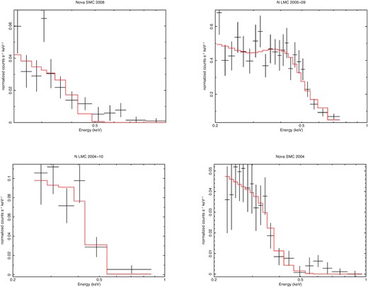
TMAP atmospheric fit to the spectra of Novae SMC 2008-10, LMC 2005-11, LMC 2004-10, and SMC 20046, at 1, 1.8, 3.9, and 5.25 yr post-outburst, respectively.
10 CONCLUSIONS
Our exploration of the N LMC 2009a X-ray high-resolution spectra has highlighted their complexity and the likely superposition of different regions of emission. We also searched the X-ray archives and discovered four more SSSs, albeit at lower luminosity than expected. These are our main conclusions.
The continuum of the spectra of N LMC 2009 indicates the supersoft emission of the atmosphere of a WD with effective temperature peaking above 810 000 K (the PION blackbody source) and likely to be around a million K (the TMAP model result), corresponding to a WD in the 1.2–1.4 M⊙ range. The continuum and its absorption edges can be well reproduced assuming only low oxygen abundance in the intervening interstellar medium and, above all, enhanced nitrogen by a factor around 100 times solar in the nova atmosphere and/or residual wind near the surface, where we assume that the absorption features originate.
The blueshift of the absorption features is explained by a mass outflow rate of the order of 10−8 M⊙ yr−1. Nova models usually assume that mass loss has ceased when the SSS emerges, but like in other novae, this does not appear to be true: some residual mass loss is still occurring.
The absorption features in this nova were never as deep (or even saturated) as in other novae served in the Galaxy and in the Clouds, as the comparison with KT Eri and with N SMC 2016 shows clearly. While the peak temperature in N LMC 2009 may have been 100 000–200 000 K hotter, implying a higher ionization parameter, the difference is so large that it is likely to have been due also to different abundances and density in the medium in which the absorption features originated.
The ejecta of this nova emitted additional thermal X-ray flux that produced a complex emission line spectrum, most likely arising from multiple regions at different temperatures, with a contribution of both photoionization and shock ionization.
Nova KT Eri seems to have a high-mass WD and a partially evolved companion in common with N LMC 2009. However, in N LMC 2009, the turn-on time was longer, and the duration of the SSS was comparable, so the ejecta initially absorbing the SSS emission may have had higher mass, but the leftover envelope was of the same order of magnitude. Since N LMC 2009a is an RN with an inter-outburst period of only 38 yr, while no outburst of KT Eri has been found in tens of years before the eruption, N LMC 2009 did not have the time to accrete comparable or higher mass before the outburst unless it had high |$\dot{m}$|, which in turn would have resulted in ejection after accretion of a small mass, unless the WD before the outburst was still relatively cool (see Yaron et al. 2005). Most likely, this nova is at only the beginning of its RN cycle with short inter-outburst periods and the WD surface has not been heated yet by a repeated outburst cycle (see Yaron et al. 2005).
The 33-s pulsation varied in amplitude and in length of the period over time-scales of hours. The search for the physical root cause of this intriguing phenomenon, already observed also in other novae, must take this fact into account.
N LMC 2009 was an order of magnitude less intrinsically luminous than the level compatible with emission arising from the whole surface. The predicted flux level was not observed in all SSS–novae, but it was indeed measured in N SMC 2016 as well as in other novae (e.g. RS Oph, Nelson et al. 2008). On the other hand, the portion of expected WD flux that is observed is much larger than in U Sco, in which only Thomson-scattered radiation was detected. We suggested that in N LMC 2009a, we observed the WD directly along the line of sight, but either dense remaining clumps in the ejecta, or a non-disrupted accretion disc, blocked the whole of the whole WD atmosphere. The clumps are a more likely explanation, because of the variability in the continuum level indicating varying visibility. The scenario we suggest is one in which part of the material, in an outflow in which instabilities occurred, was still opaque to X-rays.
We discovered that four other MC novae were serendipitously observed as SSS with low column density. There was no indication of flux variation and the absolute SSS luminosity was only about a factor of a thousand less than predicted (and indeed observed in the most luminous SSS-novae). We hypothesize that partial obscuration of the SSS was due to an accretion disc at high inclination, since these novae were detected long after the end of mass loss and it is unlikely that the ejecta still obscured the WD.
The statistics of the MC novae of the last 20 yr indicates that novae that are still SSS after 6 or more years from the outburst are rare. We also found that half of all novae were detected as SSS for at least several months between few days and 5.5 yr after the outburst. Since the sampling was done mostly at sparse post-outburst times, and it never lasted for more than a few months with Swift, or covered only one or two random epochs with XMM–Newton, the percentage of novae detectable as SSS within 6 yr from the outburst would actually be quite higher if an uninterrupted survey was possible.
ACKNOWLEDGEMENTS
M. Orio was supported by a NASA grant for XMM–Newton data analysis. A.D. was supported by the Slovak grant VEGA 1/0408/20, and by the Operational Programme Research and Innovation for the project: ‘Scientific and Research Centre of Excellence SlovakION for Material and Interdisciplinary Research’, project code ITMS2014+:313011W085, co-financed by the European Regional Development Fund.
DATA AVAILABILITY
The data analysed in this article are all available in the HEASARC archive of NASA at the following URL: https:// heasarc.gsfc.nasa.gov/db-perl/W3Browse/w3browse.pl
Footnotes
From the GAIA data base using ARI’s Gaia Services, see https://www2.mpia-hd.mpg.de/homes/calj/gdr2_distances/gdr2_distances.pdf
It yields a very similar flux distribution to the simple Poisson noise.
Also a short time before and after the exposure, to avoid boundary fitting effects, and using a step of 200 s.
We repeated the 10000 simulation process several times.
REFERENCES
APPENDIX A: SIMULATIONS OF THE AUGUST 2009 LIGHT CURVE
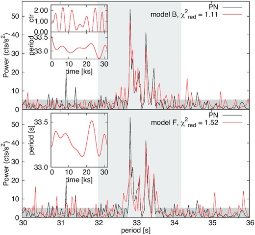
Comparison of the observed data in August and the best of 10 000 simulated periodograms for models B and F, as in Table A1. The insets show the evolution of the simulated amplitude (in count rate) and periodicity. The light shaded area is the frequency interval over which the |$\chi ^2_{\rm red}$| is calculated. The darker area represents the interval over which we calculated the power uncertainty σ (equal to the vertical extent of the shaded area).
Sine parameters of the simulated signal, amplitude (a) and periodicity (p). da and dp represent the rate of variability of the corresponding parameter (see text for details). No da or no dp values means (constant) Pa = a or Pp = p in equation (A2), respectively.
| Model | p | dp | a | da | Best |$\chi ^2_{\rm red}$| |
|---|---|---|---|---|---|
| (s) | (s) | (cts/s) | (cts/s) | ||
| A | 32.9 | 0.5 | 1.0 | 2.5 | 1.87 |
| B | 33.1 | 0.5 | 1.0 | 2.5 | 1.11 |
| C | 33.3 | 0.5 | 1.0 | 2.5 | 1.99 |
| D | 32.9 | 0.5 | 1.0 | – | 2.02 |
| E | 33.1 | 0.5 | 1.0 | – | 1.74 |
| F | 33.3 | 0.5 | 1.0 | – | 1.52 |
| G | 32.9 | – | 0.0 | 2.5 | 1.86 |
| H | 33.1 | – | 0.0 | 2.5 | 1.46 |
| I | 33.3 | – | 0.0 | 2.5 | 1.93 |
Fig. A2 shows the best case with constant periodicity but variable amplitude. However, a was set to zero, yielding the amplitude oscillate around zero and disappearing more frequently, mimicking a false beat. Larger values of a yield only a single dominant peak, which do not describe the observed feature at all. The best case reproduces all the observed features with |$\chi ^2_{\rm red}$| even better than model F. Models G and I yield single peak solutions and do not describe the complex observed pattern. Model H is acceptable, and it supports a constant periodicity P2 with variable amplitude. However, model B describes the observed periodogram much better and indicates a variable signal. With model H, we were not able to retrieve the observed power configuration, i.e. P2 having lower power than P1 and P3.4 Any periodicity introduced in the model produces the highest, or a very significant peak at the given period, while the models with variable periodicity are more flexible and appear to be more realistic. We note here that interesting periodicity evolution is shown in the upper inset of Fig. A1. Although the figure shows only a solution out of many possible ones, and an exact match is not expected, the significant decrease of the period length towards the end of the exposure is in agreement with the periodogram of the third time interval obtained when we split the exposure in three portions (see text).

The same as Fig. A1 but for model H.
