


ABSTRACT
We have simulated the evolution of non-thermal cosmic ray electrons (CREs) in 3D relativistic magneto hydrodynamic (MHD) jets evolved up to a height of 9 kpc. The CREs have been evolved in space and in energy concurrently with the relativistic jet fluid, duly accounting for radiative losses and acceleration at shocks. We show that jets stable to MHD instabilities show expected trends of regular flow of CREs in the jet spine and acceleration at a hotspot followed by a settling backflow. However, unstable jets create complex shock structures at the jet head (kink instability), the jet spine-cocoon interface, and the cocoon itself (Kelvin–Helmholtz modes). CREs after exiting jet head undergo further shock crossings in such scenarios and are re-accelerated in the cocoon. CREs with different trajectories in turbulent cocoons have different evolutionary history with different spectral parameters. Thus, at the same spatial location, there is mixing of different CRE populations, resulting in a complex total CRE spectrum when averaged over a given area. Cocoons of unstable jets can have an excess build up of energetic electrons due to re-acceleration at turbulence driven shocks and slowed expansion of the decelerated jet. This will add to the non-thermal energy budget of the cocoon.
1 INTRODUCTION
Supermassive blackholes at the centres of galaxies can launch powerful relativistic jets that can grow to extragalactic scales. These structures have since long been observed in radio frequencies, starting from observations of Cygnus A by Jennison & Das Gupta (1953). Since early days it had been established that incoherent synchrotron emission by energetic non-thermal electrons in magnetized jets gives rise to the observed radiation (Shklovskii 1955; Burbidge 1956). Subsequently, there has been extensive work to understand the physical nature of these objects (e.g. Blandford & Rees 1974; Blandford & Königl 1979) and the source of the emission. We refer the reader to reviews such as Begelman, Blandford & Rees (1984), Worrall & Birkinshaw (2006) and Blandford, Meier & Readhead (2019) for more elaborate discussions on the historical evolution of the concept of relativistic radio jets and their emission processes.
A key factor that strongly affects the emitted radiation is the nature and evolution of the non-thermal electrons inside the jet that gives rise to the synchrotron emission. It had again been identified quite early that the electrons must be energized inside the jet after ejection from the central nucleus, to avoid losing energy due to adiabatic losses in the expanding jet (Longair, Ryle & Scheuer 1973; Blandford & Königl 1979). The electrons are primarily accelerated at strong shocks inside the jet and its cocoon via diffusive shock acceleration (or Fermi 1st order processes, Blandford & Ostriker 1978; Drury 1983; Blandford & Eichler 1987). However, recent works (e.g. Rieger, Bosch-Ramon & Duffy 2007; Sironi, Rowan & Narayan 2021) have also pointed to the importance of other microphysical processes such as Fermi second order and reconnection at shear layers to accelerate particles to some extent. After an acceleration event, the energetic electrons are expected to suffer cooling due to synchrotron and inverse-Compton losses.
Detailed semi-analytical calculations of the evolution of the energy spectrum of non-thermal electron populations moving in a fluid flow have been presented in several papers (Kardashev 1962; Jaffe & Perola 1973; Murgia et al. 1999; Hardcastle 2013). However, there remain several restrictive assumptions in such semi-analytical approaches regarding the nature of the magnetic field distribution experienced by the particles, the pitch angle of the electron with respect to the magnetic field and the location of acceleration. The non-thermal electrons can experience a wide variety of physical parameters of the background environment during their trajectory, which shapes their spectrum. Addressing this requires a fully numerical approach where the non-thermal electron population are allowed to sample the local properties of the fluid, as opposed to averaged quantities.
In some recent works, numerical simulations have been presented that self-consistently evolve spectra of non-thermal electrons concurrently with the fluid (viz. Jones, Ryu & Engel 1999; Micono et al. 1999; Mimica et al. 2009; Fromm et al. 2016; Vaidya et al. 2018; Winner et al. 2019; Huber et al. 2021). The standard approach involves solving the phase space evolution of the non-thermal electrons while accounting for radiative losses and acceleration due to microphysical processes such as diffusive shock acceleration. However, such methods have been applied to study astrophysical jets in radio galaxies by only a handful of papers, and with restrictive assumptions. For example, Jones et al. (1999), Micono et al. (1999), Tregillis, Jones & Ryu (2001) have simulated the evolution of non-thermal electrons in large-scale jets but in a non-relativistic framework. Other works have evolved the non-thermal electrons embedded in relativistic fluid (e.g. Mimica et al. 2009; Fromm et al. 2016), but for small parsec-scale quasi-steady state jets, without exploring the detailed evolution up to larger distances (kpc), which is relevant for jets in radio galaxies.
In this series of papers, we will study the properties of the non-thermal electrons, evolved concurrently with the relativistic jet fluid, while duly accounting for the radiative energy losses and acceleration at shocks (Vaidya et al. 2018). The current paper, second in the series, presents the behaviour and evolution of the non-thermal electrons along with the bulk relativistic jet flow for different simulations with a wide range of jet parameters. The results on the dynamics of these simulated jets have been presented earlier in (Mukherjee et al. 2020). In subsequent papers we shall discuss the impact on observations (synchrotron and inverse-Compton) expected from such simulated jets.
The plan of the paper is as follows. In Section 2, we summarize the implementation of the method to solve for the evolution of non-thermal electrons presented in Vaidya et al. (2018) and new changes introduced in this paper in the modelling of diffusive shock acceleration. In Section 3, we discuss the numerical details of injection of non-thermal electrons. In Section 4 we briefly summarize the results of the dynamics of the simulated jets, which have been presented in detail in Mukherjee et al. (2020). In Section 5 we discuss the results of the spatial and spectral evolution of the non-thermal electrons and how they vary for different simulations with different jet parameters. In Section 6, we summarize our results and discuss on their implications.
2 EVOLUTION OF THE COSMIC RAY ELECTRONS
In Vaidya et al. (2018, hereafter BV18) a detailed analytical and numerical framework was developed to evolve a distribution of non-thermal particles both spatially and in momentum space. This was introduced as the lagrangian particle module in the pluto code (Mignone et al. 2007). This module has been applied in the current work to study the evolution of non-thermal electrons in relativistic jets. The non-thermal relativistic electrons at a region in space are modelled as ensembles of macro-particles which we refer to as a cosmic ray electron macro-particle CRE in short. The CRE are advected spatially following the fluid motions. Their energy is found by evolving their phase space distribution function, duly accounting for energy losses due to radiative processes such as synchrotron emission and inverse-Compton interaction with CMB photons. Appendix A1 briefly summarizes the method of phase space evolution of a CRE.
2.1 Diffusive shock acceleration
Electrons crossing shocks can be accelerated to higher energies via diffusive shock acceleration (hereafter DSA, see Blandford & Ostriker 1978; Drury 1983, for a review). The DSA theory predicts that particles exiting a shock can have a power-law spectrum whose index depends on the shock compression ratio defined in equation (A7). The maximum energy of the resultant spectrum is found by equating the time scale of Synchrotron driven radiative losses to the acceleration time scale (as given in equation A8). For relativistic shocks, power-law index of the spectrum is calculated differently for parallel1 and perpendicular shocks, as in equations (A10) and (A11). Further details of the above steps are summarized in Appendix A. In the next sections we describe an empirical approach to obtain the downstream spectrum of a shocked CRE.
2.1.1 Previous approaches of evaluating shocked spectra
In several previous similar works (e.g. Mimica et al. 2009; Böttcher & Dermer 2010; Fromm et al. 2016; Vaidya et al. 2018), the spectrum of shock accelerated particles were reset to a power-law with an index predicted by the theory of DSA. This would result in the particles losing the history of their spectra before the entering the shock. The normalization of the spectra and the lower limit (Emin) were set by enforcing the particles to have a fractional energy and number density of the fluid. However, this has the following two disadvantages.
In complex simulations with multiple shock features, a single computational cell may host more than one particle, and only a fraction of them may have crossed a shock. Some CRE macro-particles may have been advected to the cell without crossing a shock, by different flow stream lines. Additionally there can be multiple particles that exit the same shock feature at the same time, thus requiring a simultaneous spectral update. Hence, in a departure from Vaidya et al. (2018), where each particle was assigned an energy of fE × ρϵ, we distribute to the newly shocked particles in the cell only the energy remaining after subtracting from fE × ρϵ the existing cosmic ray energy density.
Secondly, resetting the spectrum to a new power-law results in total loss of the spectral history of previous shock encounters. Such multiple shock crossings can leave an imprint on the final spectra due to different acceleration time scales and power-law indices generated at different shocks (e.g. Melrose & Pope 1993; Micono et al. 1999; Gieseler & Jones 2000; Meli & Biermann 2013; Neergaard Parker & Zank 2014). This is especially problematic in a scenario where a particle having crossed a strong shock (higher shock compression ratio r), subsequently passes through a weaker shock with a steeper power-law index as per DSA theory. Replacing the earlier shallower spectrum with a new steeper power-law, will result in an artificial loss of energy of the CRE macro-particle.
To overcome the above limitations we introduce a empirical approach to update the spectrum of a shocked CRE, as outlined in the next section.
2.1.2 A empirical convolution based approach for updating CRE spectra
For non-relativistic shocks, equation (1) with |$\mathcal {C} = q$| and q = 3r/(r − 1), is an exact representation of the down-stream spectrum (Blandford & Ostriker 1978; Drury 1983), obtained by solving for the phase space distribution function of the particles across the shock front. In this work, we extend this as a phenomenological approach to update the up-stream spectrum of relativistic shocks. The methodology of equation (1) is similar to the implementation of reaccelerated particles in Micono et al. (1999) and Winner et al. (2019). Approximate analytical solutions of the particle distribution at a relativistic shock without an incident source predicts a power-law spectrum for the downstream particles (Takamoto & Kirk 2015). Convolving the up-stream spectrum with such a power-law distribution is thus an empirical approach that accounts for the spectrum of the incident distribution, as a CRE exits a shock. Appendix A2.2 has further details regarding the choice of the power-law index predicted from the DSA theory.
The above scheme is also similar in nature to the implementation of shock acceleration in Jones et al. (1999) and Tregillis et al. (2001), where the spectrum in an energy bin has been updated only if the index of the local piecewise power law is lower than that predicted by DSA. This duly avoids artificial steepening of spectra when energized particles with flatter spectrum crosses a weak shock, which is also naturally taken care of by the convolution process used here, as also elaborated later in this section.
The normalization constant |$\mathcal {C}$| is set in two steps, which ensure that the maximum local energy and number density of the CREs are less than or equal to a specified fraction of the fluid.
- Step 1: At computational cells where CREs are to be updated on exiting the shock, we enforce the criterion that the total energy density of all CREs in the cell should be a fraction fE of the fluid internal energy density.2 We thus first compute the total available energy in a computational volume that may be distributed amongst the newly shocked particles:Here, (ρϵ) is the fluid internal energy density, given by(2)$$\begin{eqnarray*} \Delta E = f_E \times (\rho \epsilon) - \sum _i \varepsilon _{i} , \end{eqnarray*}$$(3)$$\begin{eqnarray*} \rho \epsilon &= p/(\Gamma - 1) \quad \mbox{ (Ideal EOS)} \end{eqnarray*}$$where equation (4) is valid for the Taub–Mathews (T–M) equation of state (Taub 1948; Mignone & McKinney 2007).(4)$$\begin{eqnarray*} \rho \epsilon &= (3/2)p -\rho c^2 + \sqrt{(9/4)p^2 + \rho ^2 c^4} \quad \mbox{ (T-M EOS)} , \end{eqnarray*}$$
The energy density of a single CRE macro-particle is given by εi = ∫EN(E)dE. Freshly shocked particles that are to be updated are excluded from the summation in the second term of equation (2). For ΔE > 0, the difference in energy is equally distributed to all shocked particles in the computational cell, which sets the value of the normalization |$\mathcal {C}$| in equation (1). For ΔE ≤ 0, no new particles are updated inside the given cell, as the CRE energy density of existing particles have already reached the threshold of fE × (ρϵ).
- Step2: Subsequently, we computewhich is the difference between the fluid number density multiplied by a mass fraction fN and the total number density of all CREs in the cell, including that of shocked particles calculated in step 1 above. Here, ma is the atomic mass unit and μ = 0.6 is the mean molecular weight for ionized gas. The number density of a CRE particle is obtained from |$N^T_i = \int N(E) \mathrm{ d}E$|. For ΔN < 0, the normalization |$\mathcal {C}$| is reduced to ensure that the total CRE number density in a computational cell is Ne = fN × ρ/(μma).(5)$$\begin{eqnarray*} \Delta N = f_N \times \rho /(\mu m_a) - \sum _i N^T_i , \end{eqnarray*}$$
To summarize, the normalization is first set to preserve the energy densities of the particles to be a fraction of (fE) the fluid energy density. Additionally, if the chosen normalization results in the CRE number density becoming higher than a fraction (fN) of the fluid number density, the previously obtained normalization is lowered to ensure an exact match. In that case, the total CRE energy density will be lower than the threshold of fE × ρϵ, due to a lower value of the new normalization. Thus, the above two-step procedure ensures that the CREs have energies and number densities that are within the prescribed fractions fE and fN for energy and mass, respectively. For this work, we have assumed fE = fN = 0.1.
We must note here that chosen fractions are somewhat arbitrary, although not far from the indications obtained from PIC simulations (see e.g. Sironi, Spitkovsky & Arons 2013; Caprioli & Spitkovsky 2014; Guo, Sironi & Narayan 2014; Marcowith et al. 2016, 2020). In addition, though small, they are not negligible. In reality, CREs accelerated at shocks will subtract the corresponding fractional gain in energy from the fluid internal energy, which is not considered here. Feedback from radiative losses due to non-thermal particles can change the shock structure, as demonstrated in Bromberg & Levinson (2009) and Bodo & Tavecchio (2018). Such effects are not considered in this work as the CRE particles are considered to be passively evolving with the fluid. However, given that the CRE energy and mass fractions are restricted to a maximum of 10 per cent, the effects are not expected to be substantial, and the qualitative trends are not expected to be affected. Understanding the quantitative impact of energy losses and cosmic ray pressure requires detailed modelling of the interaction of the CRE with the fluid and will be deferred to a future work.
The above procedure to update the spectrum of a shocked CRE is better at accounting for situations where a CRE has traversed multiple shocks of different strengths. The convolution procedure introduced here (as also in Micono et al. 1999; Winner et al. 2019) will redistribute lower energy electrons to higher energy bins as per the functional form of the spectrum predicted by DSA. This may be interpreted as the lower energy electrons being accelerated to higher energies. Thus in the previously described situation of a particle passing first through a stronger shock followed by a weaker one, the resultant spectrum would be a broken power law.
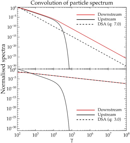
A demonstration of the empirical scheme involving convolution of the particle spectrum with the DSA predicted power-law function (in dashed). The up-stream spectrum (in black) of the particle before the shock update is a power law with an exponential cut-off given by equation (6). The resultant down-stream spectrum (in red) is obtained from their convolution.
3 NUMERICAL IMPLEMENTATION OF CRE INJECTION
We have performed a series of simulations of relativistic jets expanding into an ambient medium in Mukherjee et al. (2020, hereafter Paper I). In this section, we summarize the details of how CRE macroparticles are introduced into the simulation domain. We refer the reader to Section 2 of Paper I for details regarding the magnetohydrodynamics of the simulation and related information regarding the simulation set up.
The CRE are injected in the simulation in computational zones just above the inlet of the jet along the Z-axis, as shown in Fig. 2. Two CRE particles were injected at each cell, at each time-step, to achieve greater filling of the cocoon volume. The injected particles are immediately advected by the jet flow upwards along the jet axis. Over the course of the simulations, typically several million particles are injected, as shown by the last column in Table 1.
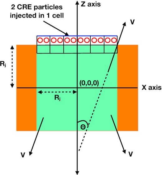
A representation of the injection zone of the jet in the simulation domain (similar to fig. 2 of Mukherjee et al. 2020), which also shows the injection of the CRE macroparticles. Two CREs, represented in red, are injected at every time-step in a computational cell (denoted by the black boxes) just above the jet inlet, along the Z-axis. The area of injection spans up to the extent of the jet radius in the X–Y plane. For one sided jets, CREs are injected only along the upper surface of the injection zone, as demarcated here. For twin jets (simulation E), CREs are injected along both upper and lower surfaces.
List of simulations and parameters.
| Sim. | γj | σB | Pj | No. particlesa |
|---|---|---|---|---|
| label | (1045 erg s−1) | (×106) | ||
| Bb | 3 | 0.1 | 0.2 | 16.4 |
| D | 5 | 0.01 | 1.1 | 6.5 |
| E | 5 | 0.05 | 1.2 | 18.0 |
| F | 5 | 0.1 | 1.2 | 3.2 |
| G | 6 | 0.2 | 8.3 | 14.9 |
| H | 10 | 0.2 | 16.4 | 9.8 |
| J | 10 | 0.1 | 15.1 | 55.3 |
The total number of particles injected during the course of the simulation.
The density contrast defined as the ratio of the jet density to ambient gas is 4 × 10⁻⁵. For all other cases, the value is η = 10−4.
Parameters:
γb: Jet Lorentz factor.
σB: Jet magnetization, the ratio of jet Poynting flux to enthalpy flux. See equation (7) of Paper I.
Pj: Jet power. See equation (9) of Paper I.
However, one must note that the starting configuration of the CRE spectrum defined in equations (7) and (11) is renewed when they encounter the first shock, which occurs fairly close to the injection surface, from the recollimation shocks within the jets. Thus, the resultant spectra of the particles inside the main jet flow after some distance away from the injection surface are insensitive to the initial values.
4 REVIEW OF RESULTS FROM PAPER I
In Mukherjee et al. (2020, Paper I) we have presented the results of the simulations of relativistic jets, focusing on the evolution of the dynamics and fluid parameters in the jet and its cocoon. Table 1 lists the simulations where the non-thermal CREs were evolved along with the fluid. We keep the same nomenclature of the simulations as done in Paper I, for consistency. The simulations probe a wide range of jet parameters, namely: jet power (Pj), jet magnetization (σj), and the bulk Lorentz factor (γj). Broadly we can divide the results into three groups: simulation B with a low power jet (Pj ∼ 1044 erg s−1), simulations D, E, F with moderate power jets (Pj ∼ 1045 erg s−1), and simulations G, H, J with high power jets (Pj ∼ 1046 erg s−1). In most simulations, the jets were followed up to 9 kpc, except for simulation J where the domain is larger.
In Paper I, we have discussed the dynamics of the jets. One of the primary results of the paper, which is also strongly relevant for the discussion in the current work, is the onset of different MHD instabilities for different ranges of jet parameters. We summarize briefly below the main findings of Paper I which are relevant to this work.
Kink unstable (simulation B): Simulation B with a low power jet (Pj ∼ 1044 erg s−1) and strong magnetization (σB ∼ 0.1) is unstable to kink mode instabilities. The kink instabilities cause the jet axis and head to bend strongly, which creates complex shock structures at the jet head (see fig. 4 in Paper I).
KH unstable (simulation D): Jets with lower magnetization, such as simulation D with Pj ∼ 1045 erg s−1 and σB = 0.01, suffer from Kelvin–Helmholtz (hereafter KH) instabilities. This decelerates the jet and creates turbulence inside the jet and cocoon, with a disrupted jet spine due to vortical fluid motions resulting from the KH modes.
Stable jets (simulations F and H): Moderate to high power jets (Pj ∼ 1045–1046 erg s−1) with stronger magnetization (σB ∼ 0.1) remain stable to both kink and KH modes up to the run time of the simulations explored in these works, such as simulations F and H. This is due to reduced growth rates of KH modes due to stronger magnetic field and also reduced growth of both kink and KH modes due to higher bulk Lorentz factors.
Turbulent cocoon (simulation G): Higher pressure of the jet results in more internal structure. The higher sound speed facilitates the growth of small-scale perturbations (Rosen et al. 1999), which can develop internal shocks and turbulence. Simulation G (Pj ∼ 1046 ergs−1) with an injected jet pressure five times that of simulation H, shows such internal instabilities and turbulence.
In the rest of the paper, a major theme would be to explore the effect of the above different MHD instabilities on the evolution of the CREs.
5 RESULTS
According to the standard evolutionary picture, CREs are considered to be carried by the jet up to the termination shock at the jet head, and eventually follow the back-flow in the cocoon to lower heights, as shown in Fig. 3. The particles are expected to be accelerated to high energies with a shallow power-law spectrum at the jet head and subsequently cool down in the backflow inside the cocoon due to radiative losses from synchrotron and inverse-Compton interaction with the CMB radiation (Jaffe & Perola 1973; Murgia et al. 1999; Hardcastle 2013; Harwood et al. 2013; Harwood, Hardcastle & Croston 2015). However, the above picture is simplistic, especially for complex flow patterns arising out of MHD instabilities in the jet and the cocoon. In the following sub-sections, we describe the behaviour of the particles as they evolve with the jet and highlight the differences from the above standard paradigm.
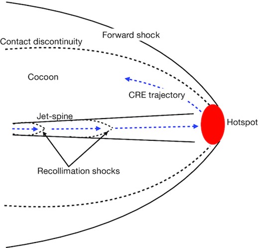
A schematic showing the structure of the jet spine, the cocoon surrounding it, the contact discontinuity, and the forward shock. The non-thermal electrons (called here as CREs) are expected to travel first through the jet spine up to the hotspot and flow back down into the cocoon. The CREs are first accelerated at the sites of recollimation shocks (Norman et al. 1982; Komissarov & Falle 1998) inside the jet before they reach the strong shock at the hotspot.
5.1 Evolution of CREs in the jet and cocoon
5.1.1 CREs in stable powerful jets
In this section, we describe the coevolution of the CREs with the jet for case H, a prototypical stable jet with Pjet = 1046 erg s−1. The CREs injected at each time-step (as outlined in Section 3) are advected along with the jet flow till they reach the jet head. There, the CREs interact with the termination shock and turn back into the cocoon pushed by the jet’s back-flow. This is well demonstrated by the trajectories of four representative CREs in Fig. 4. The chosen particles from four different heights at the end of the simulation have the largest number of shock crossings at the given heights.
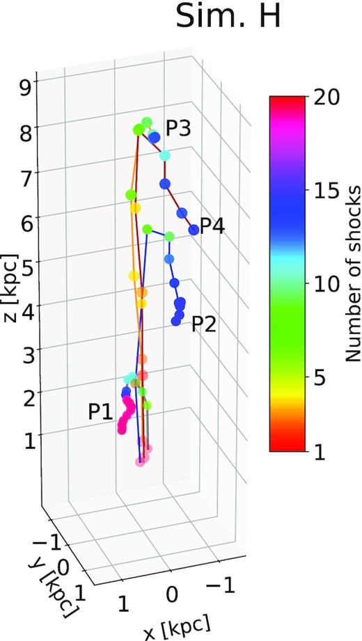
Trajectories of four representative particles (named P1, P2, P3, and P4) that undergo multiple shocks in simulation H. The colour of the particles shows the number of shocks crossed at a given point of the track.
The CREs are first accelerated inside the jet spine itself, at the several recollimation shocks, before they reach the jet head. This causes the particles to attain a large value of maximum Lorentz factor γmax inside the jet axis. This can be seen in the top panel of Fig. 5, where we present the CREs with colour scaled to the value of log (γmax), overplotted on the density profile in the Y–Z plane. The bottom panels of Fig. 5 show the particles coloured by time lapsed since last shock encounter. The CREs within the jet axis are also seen to be young in age as they have been relatively recently shocked at the sites of recollimation.
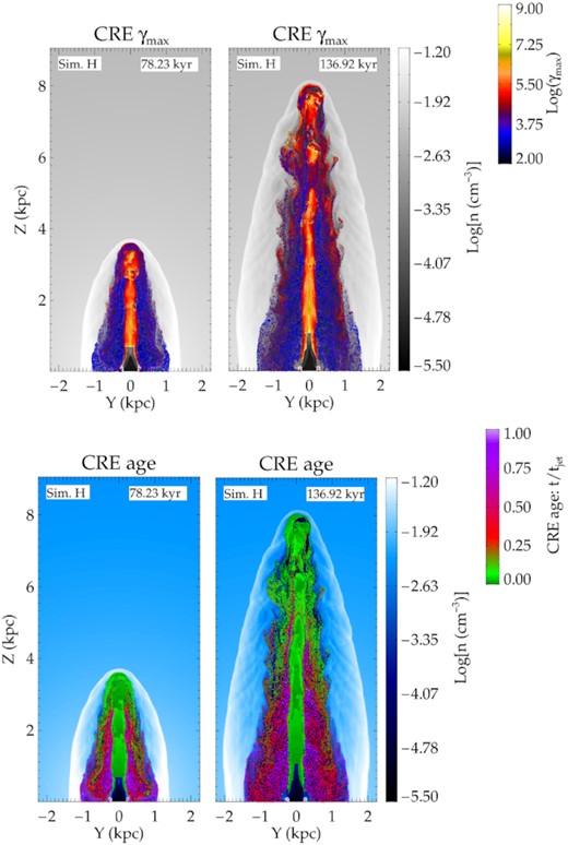
Top panels: Density slices in the X–Z plane for simulation H at two different times. Overplotted on the density maps are particles with colours representing the log (γmax), where γmax is the highest Lorentz factor of the CRE spectrum. Bottom panels: Density slices in the X–Z plane with the CRE positions overplotted. The colour of the CRE represents the time since last shock, normalized to the time of the simulation. Freshly shocked particles (greenish hue) are near the jet head, with older particles (purple/pink) at the base.
Once the particles reach the jet head, they cross the strong shock at the Mach-disc and follow the backflow of the jet into the cocoon. The cocoon has older particles represented in magenta and red in Fig. 5. The CREs in the cocoon also have lower maximum energies as they lose energy steadily due to radiative losses. Thus, the CREs in this simulation of a jet stable to MHD instabilities conform well to the standard evolutionary picture proposed in earlier works (e.g. Jaffe & Perola 1973; Komissarov & Falle 1998; Turner & Shabala 2015), as also summarized in the schematic in Fig. 3.
5.1.2 Impact of MHD instabilities
Simulation B, kink unstable: Simulation B with a lower jet power (Pj ∼ 1044 erg s−1) shows a uniform distribution of maximum Lorentz factor, as shown in the upper panel of Fig. 6. This is in sharp contrast to that of simulation H (Fig. 5), where the high values of γmax are concentrated at the locations of the strong shocks in the jet axis and the jet head. The kink instabilities result in the bending of the jet head, ultimately leading to the formation of an extended termination shock spreading horizontally from the main axis of the jet (see top panel in Fig. 7). CREs traversing such shock will undergo complex shock crossings. For example, the paths of P1 and P3 are sharply twisted as they encounter the complex shocks at the jet head. They undergo several shock crossings after they exit the jet axis, evidenced from the rapid change in the colour in the lower panel of Fig. 6.
The instabilities also strongly decelerate the jet. This results in constant injection of energetic CREs into the slowly inflating cocoon. CREs exiting the jet at different heights lie close together near the base (e.g. particles P2 and P3). Such CREs are further reaccelerated at other shock surfaces due to internal turbulence and the complex backflow. For example, particle P3 (right-hand panel of Fig. 6) gets further shocked after exiting the jet axis due to internal shocks inside the cocoon. Thus, there is mixing of particles with different shock histories, and the cocoon of a decelerating slowly inflating jet is more evenly distributed with shocked highly energetic particles.
Simulation D, KH unstable: Simulation D with KH instabilities has multiple internal shocks inside the cocoon, as shown in the 3D volume rendering of the shocks in Fig. 7. The shock surfaces are identified by computing the maximum pressure difference at each grid point, as defined in equation (A5). Similar complex web of shock structures have also been reported in Tregillis et al. (2001). CREs streaming down the backflow will have to cross these shocks and be reaccelerated in the process. CREs shocked multiple times are trapped within this shock layers.
The above situation is clear by inspecting the complex trajectories of the CREs in the left-hand panel of Fig. 8, where the paths of two representative CREs have been plotted. CRE P1 with the particle trajectory presented in red lines connecting the locations at different times, is seen to perform a loop at Z ∼ 3 kpc, before reaching to a maximum height of Z ∼ 5 kpc and subsequently streaming down. CRE P2 similarly shows a complex trajectory (in blue) with a vertical rise up to Z ∼ 6 kpc, a backward motion thereafter, and again a rise up to Z ∼ 8 kpc. These vortical motions of the CREs result from the onset of KH instabilities at the jet–cocoon interface.
What is noteworthy here is that the cause for the multiple shock crossings in simulation D is fundamentally different than that in simulation B. In simulations B and H, the CREs are shocked multiple times due to the geometry of the shock structure at the jet head, beyond which they stream down along the back flow, with some exceptions. The CREs in simulation Dencounter multiple weaker shocks within the body of the cocoon itself as they stream down along the backflow and also at the outer layer of the jet spine where KH driven vortices arise, leading to turbulence and shocks.
Thus a more extended region of the cocoon is filled with freshly shocked younger electrons, as shown in middle panel of Fig. 8. Similarly from the right-hand panel of Fig. 8, it can be seen that the CREs inside the cocoon are shocked to higher energies, in sharp contrast to that in simulation H (Fig. 5). This is because the magnetic field in simulation D is almost an order of magnitude lower than that in H, resulting in longer synchrotron cooling time-scales (see equation A8), allowing efficient acceleration.

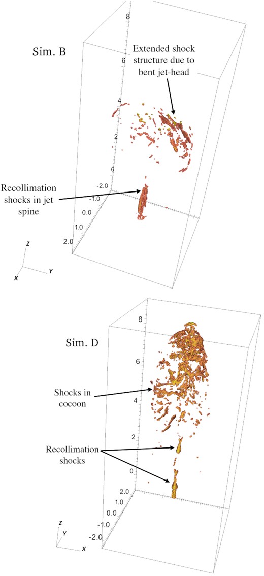
A 3D volume rendering of shocked surfaces in the cocoon of simulations B (top) and D (bottom). The shocks are identified by the Δp/p > 3, as described in Section 5.1.2. The spatial scale of the axes is in kilo-parsecs.
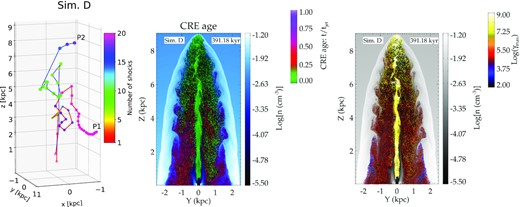
Left: Tracks of two representative CREs in simulation D. The track of P1 is shown by a red line connecting its locations at different times. Similarly, the track of CRE P2 is represented by the blue line connecting the dots. The colour of the dots denotes the number of shock crossings experienced (as also in Fig. 4). Middle: The density slice for simulation D with particle colour showing age since last shock, as in the lower panel of Fig. 5. Right: Density slice, with particle colour showing log (γmax), as in the upper panel of Fig. 5. A larger portion of the cocoon has freshly shocked particles due to turbulence generated shocks in the cocoon depicted in the left-hand panel.
5.2 History of the magnetic field, γmax, and shock compression ratio traced by CREs
MHD instabilities can create turbulence in the jet cocoon, resulting in inhomogeneous distribution of magnetic and velocity fields. Thus, depending on their trajectories in the jet–cocoon, different CRE particles may experience varied evolutionary history. In Fig. 9, we present the variation of the magnetic field, the maximum Lorentz factor of the CRE spectrum (γmax), and the shock compression ratio of the last shock crossed, for some of the representative particles already shown in Fig. 4, 6, and 8. The variation of these quantities along the CRE trajectory will leave their imprint on the CRE energy spectrum.
Simulation B: The left column of Fig. 9 shows the evolution of physical properties for particles P2 and P3, whose trajectories have been presented in Fig. 6. We firstly notice that although the two particles have similar trajectories, they encounter very different magnetic fields. Particle P3 shows a sharp increase to about ∼0.2 mG, followed by a decline, and similar subsequent spikes, although of lower magnitudes. The rapid increase in the magnetic fields correlates well with changes in the shock-compression ratio, indicating that such sudden increase results from the CRE traversing different shocks during its trajectory. The γmax also shows similar correlated increase to high values, followed by an exponential decline after the last shock. It is interesting to note that since its injection after ∼650 kyr of the simulation run time, CRE P3 experiences multiple shocks for ∼200 kyr, before entering a steady quiescent backflow without shocks. This is due to the complex shock structure created by the kink unstable bending jet head.
CRE P2, however, experiences a very different evolution, with a steady magnetic field fluctuating about a mean of ∼0.04 mG. The γmax shows some initial increase as the CRE travels through the jet axis and reaches the complex shock at the jet head, as also corroborated from the initial changes in compression ratio. However, post jet exit, the CRE streams through the backflow with an exponential decay of γmax. The evolution of P2 is thus along the lines of the standard expectation of CRE evolution proposed in traditional analytical models (Jaffe & Perola 1973; Turner & Shabala 2015), as also depicted in Fig. 3. However, CRE P3 with multiple shock crossings spread over a long duration, is a result of the local inhomogeneities due to non-linear MHD.
Another point to note is that, the high γmax of CRE P3 coincide with high values of the compression ratio (r > 1.5). This is expected, as strong shocks of higher compression ratio (r), will give rise to higher values of γmax for the same strength of magnetic field, as can be seen in equations (A8) and (A9). However, for CRE P2, the initial rise in γmax corresponds to crossings of weak shock (r ≲ 1.3), and also lower magnetic field strengths than P3 by nearly an order of magnitude. As can again been seen from equation (A8), lower values of magnetic field strength at shocks will also result in an increase in γmax due to lower synchrotron cooling times. Thus, these two CREs demonstrate well how CREs can experience different physical conditions during their trajectory, and how they differently affect their spectra.
Simulation D: For simulation D (middle column of Fig. 9), we present the results for CREs P1 and P2 labelled in Fig. 8, which have very different spatial tracks, as discussed earlier in Section 5.1.2. The turbulent magnetic field fluctuating on smaller length-scales than other simulations results in the CREs experiencing a magnetic field fluctuating about a mean value (∼0.04 mG) as well. The γmax, however, shows sharp increase followed by phases of decline. The increase in γmax correlates with an increase in the compression ratio, indicating that the particles have traversed through strong shocks with compression ratios r ≳ 2 − 4. The multiple peaks in the γmax at different times result from re-acceleration at internal shocks during their motion within the cocoon. The low mean injected magnetic field in this simulation, also contribute to the high values of γmax.
Simulation H: For simulation H, we present the results for 3 CREs. CRE P1 exits the jet at Z ∼ 3 kpc and proceeds laterally onwards into the cocoon. CREs P3 and P4 injected at later times exit at a higher height (Z ∼ 9 kpc). As CRE P1 proceeds through the jet axis, it experiences an initial rise of magnetic field along its trajectory, followed by a lower value of ∼0.1 mG. CREs P3 and P4 having been injected at similar times, follow similar trajectories and show a similar nature of the time evolution of the magnetic field and shock compression ratio. The initial γmax of P3 is higher as it likely passes through a stronger recollimation shock after injection, than P4.
Although the CREs experience stronger shocks than simulation D, the γmax is not much higher than that in simulation D. The stronger magnetic field in simulation H causes faster radiative losses of the CREs reducing the efficiency of shock acceleration.

5.3 Multiple internal shocks
As stated earlier in previous sections, MHD instabilities create complex shock structures inside the jet cocoon where CREs can be reaccelerated. Fig. 10 shows the probability distribution function (hereafter PDF) of the number of shocks encountered by CREs in different simulations. Simulations with similar power are plotted with same linestyles although different colours viz. simulations D (green) and F (brown) with Pjet ∼ 1045 erg s−1 in dashed, and simulations G (blue) and H (red) with Pjet ∼ 1046 erg s−1 in solid. KH instabilities in simulation D result in higher number of shock crossing with the PDF showing a very extended tail than that in others. Similarly, simulation G that has more internal structures and shocks due to higher internal sound speed has a slightly extended PDF than the stable jet in simulation H. Simulations F and H show a slight hint of bi-modality. This results from joint contributions of the CREs in the jet spine which are shocked only at a few recollimation shocks and the CREs in the cocoon which have been shocked many times at the jet head or the internal shocks in the cocoon.

The distribution of number of shocks traversed by the particles during their lifetime for simulations B, D, F, G, and H. Stable jets in F and H have steep tail due to lower shock crossings. Simulation D with KH modes has an extended tail indicating many crossings.
5.4 Maximum Lorentz factor of CREs
5.4.1 Distribution of γmax at different heights
In this section, we discuss the effect of multiple shock encounters on the maximum Lorentz factor of the CREs (γmax), which is defined by equation (A8). Fig. 11 shows the PDF of the γmax at three different heights, corresponding to the jet head (∼7 kpc, in blue), the middle zone (∼5 kpc, in brown), and the base of the cocoon (∼3 kpc, in black), for different simulations. The PDFs at different heights are instructive to understand the evolution of the CRE spectra, as they are shocked at the jet head and later again while crossing weaker shocks in the back flow.

The distribution of γ for different simulations, at three different heights, following the convention of Fig. 10. The three panels correspond to simulations of in three ranges of power. The PDFs in general show a peak (which is well described by a lognormal distribution shown in dashed lines), followed by an extended tail to high γ.
First, it is evident that the PDFs have a more extended distribution (γmax ∼ 109) closer to the jet head (∼7 kpc), where they encounter the strong terminal shock. The PDFs in the mid-planes for simulation B have a lower value of maximum Lorentz factor (γmax ≲ 108) as they consist of particles that have cooled due to radiative losses. However, in simulations D and G, γmax in the middle zone extends up to γmax ∼ 109 as particles get reaccelerated by internal shocks inside the cocoon.
The PDFs have a general nature of a peak at γmax ∼ 105, followed by an extended tail. The peak and the lower end of the PDF are often well described by a lognormal distribution, as shown by the dotted lines in Fig. 11. The peak of the lognormal shows a decreasing trend with distance from the jet head, indicating radiative losses. The tail of the PDF extending beyond the lognormal to high Lorentz factors (γmax ∼ 108–109), comprizes of freshly shocked electrons. Such particles thus form a different population of highly energetic, freshly shocked electrons. The PDF at ∼7 kpc for simulation F (middle panel, in red) indeed shows a bi-modal distribution with the higher peak also described by a lognormal like distribution.
5.4.2 Multiple shocked components
The onset of MHD instabilities creates different population of CREs with different shock histories and energetics. This can be seen from the 2D PDFs of the number of shock crossings of the CREs and the γmax in Fig. 12. The PDFs have been made at a height of z = 5 ± 0.2 kpc, which is approximately half the jet height at the end of the simulation. The half height was selected so that CREs have enough time to settle into the backflow inside the cocoon, after exiting jet.
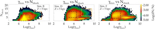
2D PDF of γmax versus number of shocks crossed (Nshock) by a CRE macro-particle at a height z = 5 kpc at the end of the simulation. Three different CRE populations have been highlighted in coloured boxes. (1) Pop. I in the black box: Older CREs with decayed spectra. (2) Pop. II in green box: Freshly shocked CREs with high energies that lie in the jet spine. (3) Pop. III in orange box: reaccelerated CREs that have been shocked many times.
We can see that in general three zones can be identified, for three different populations of CREs:
Pop. I: They are represented approximately by the blackbox in dash–dotted contours, overplotted on the PDF maps in Fig. 12. Such CREs have experienced 5–10 shock crossing (lower for simulation B) and have γmax ∼ 104–106, peaking around γmax ∼ 105. This is typical for CREs whose higher energy part of the spectra is decaying due to radiative losses. The mean spread of γmax of these CREs corresponds well with the peak of the lognormal distribution at ∼5 kpc in Fig. 11 discusses earlier. Thus these CREs represent the bulk of the non-thermal electrons in the cocoon whose spectrum follow the standard evolutionary scenario of being accelerated at the jet head and followed by radiative cooling, as shown in the cartoon in Fig. 3.
Pop. II: There is a second population of CREs, especially for simulations D and F, with high energies (γmax ∼ 107–109), but less number of shock crossings (Nshock ∼ 2–5). They are highlighted by a green box with dashed contours in the middle and right-hand panels of Fig. 12. These are CREs in the jet spine, which have been energized by recollimation shocks, and hence the high γmax. Since, there are only a few of recollimation shocks in the jet, they have undergone only a handful of shock crossings.
Pop. III: A third population of CREs can be identified in simulations B and D, which have high γmax ∼ 107–109 and multiple shock crossings (Nshock > 5), denoted by the orange box in the left and middle figures of the top panel in Fig. 12. These CRE have crossed multiple shocks either in the complex structure at the jet head (as in simulation B) or internal shocks inside the cocoon (e.g. simulation D). This is a signature of jets with active MHD instabilities, and is distinctly absent in simulationF, which is stable to both kink and KH modes, as also reported recently in Borse et al. (2021). In simulation F, after crossing the jet head, the CREs cool down in the backflow, without being reaccelerated, unlike the CREs in Pop. III category.
5.5 Distribution of CRE ages at a given height
The cocoon has a wide distribution of CRE ages due to their different propagation history. This is accentuated in a turbulent jet where regular streamlines inside the backflow are disrupted due to instabilities. In Fig. 13, we present the 2D distribution of γmax and the CRE age since injection into the computational domain, normalized by the simulation run-time. The PDFs have been constructed by extracting all particles at a height of Z = 5 ± 0.2 kpc, which includes both particles within the jet spine and the cocoon. The above has been performed for simulations D and F, at the end of the respective simulations, when the jet has reached a height of ∼9 kpc, such that the height chosen to extract the CREs approximately represents the middle of the jet–cocoon structure.
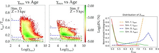
Left and middle: 2D PDF of γmax versus time elapsed since a CRE is injected (tage) representing the age of a CRE in the simulation, normalized to the total simulation time (Tsim). The green box denotes CREs inside the jet. The green-dashed line denotes the time to reach z = 5 kpc with a speed c, normalized to the simulation time. The blue lines marked by tL and tU denote the extent of the distribution of ages within the cocoon that have exited the jet. See text in Section 5.5 for further details. Right: The distribution of maximum height (Zmax) reached by particles with the ages tL and tU in the previous panels.
We firstly notice a bi-modal distribution, with the lower values in the green box representing CREs inside the jet. These CREs have been recently injected, and hence the low age. They travel at near light speed up to a height of ∼5 kpc, as can be seen from the green horizontal lines in the figures, showing tage = 5 kpc/(cTsim), where Tsim is the end time of the simulation. The above line represents the lower end of the distribution, with the rest of the particles being older owing to slower propagation speed inside the jet axis.
Above the CREs in the jet beam, there is an extended distribution of CREs, which represent the CREs inside the cocoon.The cocoon CREs at ∼5 kpc cover wide range in ages, demarcated by the two limits, tL and tU, respectively, as denoted in the figure. The upper limit, tU, from the oldest CREs at Z = 5 kpc, corresponds to particles that have exited the jet spine when the jet head had reached a height of ∼5 kpc during its evolution, and have remained at the similar height up to the end of the simulation. In the regular back-flow model, one would expect the CREs to then stream downwards into the cocoon. However, several CREs follow complex trajectories, which are often lateral, as also shown in Figs 6 and 8. These CREs hover around the original height from which they had exited the jet, which likely result from internal turbulent flows. Being older, they also have a lower value of γmax ≲ 107, due to radiative losses. The lower limit, tL, corresponds to CREs that have exited the jet at a more recent time, when the jet has evolved to a larger height, and subsequently travelled downwards to Z ∼ 5 kpc with the backflow.
Estimates of tU from equation (12).
| Sim. | t* | Tsim | vj/c | tage/Tsim |
|---|---|---|---|---|
| label | (kyr) | (kyr) | ||
| D | 205 | 391 | 0.35 | 0.6 |
| F | 166 | 235 | 0.7 | 0.39 |
| Sim. | t* | Tsim | vj/c | tage/Tsim |
|---|---|---|---|---|
| label | (kyr) | (kyr) | ||
| D | 205 | 391 | 0.35 | 0.6 |
| F | 166 | 235 | 0.7 | 0.39 |
Similarly, to model the ages of the CREs at tL, assuming (vj, vb, vh) ≡ (0.9, 0.3, 0.065)c for simulation D, gives tage ∼ 0.13Tsim, for the chosen height of L = 5 kpc. This is close to the observed limit in Fig. 13. Similarly, for simulation F, the choice of (vj, vb, vh) ≡ (0.9, 0.3, 0.1)c gives tage ∼ 0.18Tsim. The above choices though ad hoc, are reasonable in their values and are indicative of the nature of the CRE motion in the backflow. In Fig. 14 we show the Z component of the velocity, depicting the velocity in the jet as well as the backflow. It can be seen that the choice of vj ∼ 0.9c and vb ∼ 0.3c are within limits of the actual values inferred from the velocity maps in Fig. 14. A smaller value of vh is used for simulation Dto account for the decelerated jet advance due to KH instabilities. The value used is consistent with the mean advance speed of the jet presented in fig. 15 of Mukherjee et al. (2020).
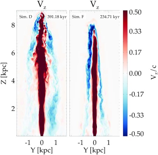
The vz component of the velocity field (normalized to c) for simulations D and F. Simulation F shows an extended backflow that remains mildly relativistic (∼0.3–0.5c) for a major part of the cocoon. For simulation D, the backflow loses momentum after a few kpc from the current location of the jet head.
An interesting point to note is the nature of the distribution of maximum heights reached by CREs with tage = tL for simulations D and F, as shown in the right-hand panel of Fig. 13. While simulation F has a sharp peak at Zmax ∼ 7 kpc, similar CREs in simulation D has a broader distribution, ranging between ∼6 and 8 kpc. This points to the fact that simulation F being stable to MHD instabilities, has a regular, well-defined backflow, as can also be seen in Fig. 14. However, MHD instabilities in simulation D disrupt the backflow resulting in intermittent flow patterns and mean speed for different CRE stream lines. This results in a wider distribution of CREs of different ages at a given height.
5.6 Evolution of CRE spectrum
5.6.1 Spectrum as a function of time for a single CRE
The spectrum of a CRE macro-particle changes in the simulation due to two reasons: (i) shock encounters that accelerate the electrons and (ii) radiative losses due to synchrotron or inverse-Compton emission. Losses due to inverse-Compton interaction with CMB are nearly constant at all locations, and secondary to synchrotron driven cooling for strong magnetic fields (B ≳ BCMB, as in Ghisellini et al. 2014). For the simulations explored in this work, the magnetic field is well above the critical field. Fig. 15 shows the evolution of the spectrum of particle P1 of simulations D whose trajectory has been shown in Fig. 8. The figures show how the spectrum changes after the particle has experienced multiple shock encounters.
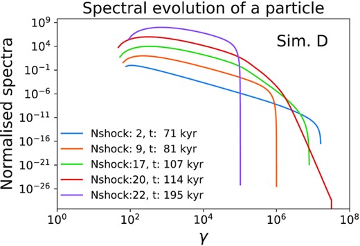
The evolution of the spectra for particle P1 in simulation D from Fig. 8. The legends show the number of shocks crossed and the simulation time for each spectrum. The spectra are normalized to their maximum value. Each spectrum is offset vertically by a factor of 100 from the one below for better visual representation.
At the initial stages, the spectra are well represented by a power law with a sharp cut off due to cooling losses, as expected from a cooling population of shocked electrons (Harwood et al. 2013). However, the energy distributions at the intermediate times are not described by a simple power law with an exponential cut-off. Some of the spectra have a curved shape, well approximated by piecewise power laws (e.g. the red and green curves). Such an evolution may arise when multiple shocks of varying strengths are encountered, as was demonstrated in the top panel of Fig. 1, in Section 2.1.2. However, the high-energy tail will eventually decay with time and the softer slopes from the strongest shock encountered during the particle’s history will set the slope at lower energies. Eventually the spectra at end (purple curve) can be approximated as a power law with an exponential cut-off.
5.6.2 Average CRE spectrum at different locations
CREs have significant difference in spectra depending upon their shock crossing histories during their trajectory due to internal turbulence in the cocoon. The resulting spectra of a collection of non-thermal electrons over a region can thus strongly deviate from a power law with a sharp cut-off. We demonstrate an example of this in Fig. 16, where we show the total particle spectra centred at three locations in the Y–Z plane. Particles in a volume consisting of an area of 200 × 200 pc2 in the Y–Z plane and the entire X-axis are then extracted and their spectra summed and plotted in Fig. 16. The first two locations (S1, S2) represent the spectra expected from the cocoon and the jet axis, respectively, at Z ∼ 5 kpc. The third location (S3) samples the spectra from a region near the jet head.
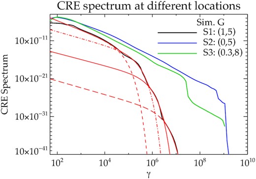
The total CRE spectra of particles at three different locations for simulation G at the end of its runtime. The coordinates (in kpc) of the centre of the chosen locations in the (Y–Z) plane are presented in the figure legend. The black and blue curves are centred at the cocoon and the jet, respectively. The green curve is near the jet head, slightly off-centred from the Z-axis. The three red curves in dashes and dots are representative power laws with exponential cut-offs, with the parameters in Table 3, whose envelope given by the red solid line well approximates the spectrum of P1 (in black). See text in Section 5.6.2 for further details.
The locations S2 and S3 being near the jet axis have their spectra extended to γ ∼ 109 as the CREs are accelerated inside the jet. On the other hand, the location S1, sampling the cocoon, has a decaying spectrum (in black). The decay in the spectrum is not a sharp exponential cut-off as often expected for cooling electrons (Harwood et al. 2013, 2015), and also seen for single electrons in Fig. 15. Instead, one can identify clear bends in the spectra which are indicative of a superposition of different electron populations, with different shock and cooling histories. We overplot in red four representative power-law curves with exponential cut-offs following equation (6). The parameters are listed in Table 3. The curves have different cut-off Lorentz factors indicating difference in cooling time-scales, and slightly different power-law index implying different shock crossing histories. The superposition of these individual components, which we reiterate is not an actual fit, represents well the final spectrum.
This indicates that the spectrum of a region in the cocoon will have imprints of different electron populations, which arise out of different evolutionary histories of the CREs in a turbulent cocoon. A similar such imprint of multiple electron population is seen in for S3 at Z ∼ 8 kpc of Fig. 16. It clearly has two components, with a slightly older population having a cut-off Lorentz factor at γ ∼ 107.5, and another population of shocked electrons extending as a power law up to γ ∼ 109. Since the location of S2 is close to the jet axis, the sum of the spectra of all CREs along the X-axis will consist of CREs both inside the jet axis, as well as the intervening cocoon with backflow. The resultant spectrum gives a complex shape with two distinct populations, one slightly cooled in the cocoon and the other from the jet spine. Similarly, also at location S2, we observe the presence of two components, with cut-offs that are, however, at quite close values of the Lorentz factor.
5.7 Particle energy distribution
An important ingredient in modelling the evolution and emission from lobes and jets of radio galaxies is the inherent assumption that the energies in fluid enthalpy, magnetic field, and non-thermal particles are in approximate balance, the so-called equipartition argument (Hardcastle et al. 2002; Croston et al. 2005; Worrall & Birkinshaw 2006; Ineson et al. 2017). Although a convenient assumption in most cases, it is unclear whether such a balance is actually reached and to what extent jet parameters and fluid instabilities can affect it. We present in Fig. 17, the evolution of the volume-averaged values of the three different energy components in the jet and cocoon separately. The relativistic fluid enthalpy is given by ρh = ρc2 + ρϵ + p, where the internal energy (ρϵ) for a Taub–Matthews equation of state is given by equation (4). The values are computed from a time when the jet height is larger than Zj ≳ 1 kpc. The regions with jet tracer between 10−7 ≲ Tracer ≲ 0.8 is considered to be the cocoon, and the volume with Tracer ≳ 0.8 is considered to be the jet.
Jet beam: We first note that inside the jet, the fluid enthalpy dominates over both components. The magnetic field and the fluid enthalpy maintain a steady difference for all simulations. The particle energy is comparable to the magnetic field energy, but lower than the fluid enthalpy by an order of magnitude or more. This is by design, and results from the choice of fE = 0.1 to be enforced at the shocks, as described by equation (2) in Section 2.1.2. However, simulation D shows some noticeable difference. It is to be noted that simulation D has a lower magnetization (σB = 0.01) and hence a lower magnetic energy density to start with. Thus, the CRE energy is higher than the magnetic field initially, although close to ∼0.1 of the enthalpy. However, over time, the particle energy decreases and becomes comparable to the magnetic field energy inside the jet.
Cocoon region:
Stable jets: In simulation F(right-hand panel of Fig. 17), the particle energy is again lower than the fluid enthalpy and maintains a steady difference, as in the jet. This is because the particles are shocked at the jet head and stream down with the backflow and cool in the cocoon. The particle energy density is further diluted by the expansion of the cocoon volume due to the rapid advance of the jet. This is typical of the standard expectations of evolution of an FRII jet (Jaffe & Perola 1973; Turner et al. 2018).
Unstable jets: Inside the cocoon of unstable jets such as the kink unstable simulation B (left-hand panel) and the KH unstable simulation D (middle panel), the particle energy can become comparable to the fluid enthalpy. For simulation B this results from the following two effects: (i) the particles are strongly energized by an extended shock due to the bent jet head at different times; (ii) instabilities slow down the jet advance speed and the cocoon is continuously fed with energetic particles, which may be further shocked due to internal turbulence. Thus, low power unstable jets with slow advance speed can have increased CRE energy density.
Similarly, in simulation D (middle panel of Fig. 17), the particle energy shows an initial decline followed by an increase to become comparable again to the fluid enthalpy. The initial decline results from the adiabatic expansion of the cocoon as the jet advances. The subsequent rise occurs after the onset of the KH instabilities, when the jet has grown sufficiently. The instabilities both slow down the jet advance and accelerate the CREs at shocks due to the ensuing turbulence, which results in pumping of energetic CREs into the cocoon. This makes the CRE energy density eventually become comparable to the fluid enthalpy itself.
It is to be noted that in the jet beam, where the CRE encounter strong shocks, the enthalpy always exceeds the particle energies. This follows from our imposed constraint of the CRE energy being a fraction of the internal energy (fE = 0.1) at shocks. However, in the settling backflows, the cocoon of unstable jets can have an excess build up of high-energy CRE due to slow expansion of the cocoon and reacceleration at internal shocks.
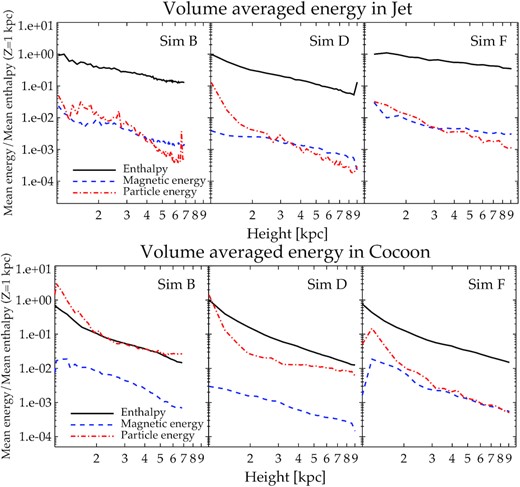
The evolution of the volume averaged enthalpy (black), magnetic energy (blue dashed), and particle energy (red dash–dotted) with jet height for three simulations. Top: The values computed for the jet (JetTracer ≳ 0.8). Bottom: The energy components for the cocoon (10−7 ≲ JetTracer ≲ 0.8). The curves have been normalized to the starting value corresponding to the jet height Z ∼ 1 kpc.
The distribution of the different energy components inside the jet is shown more explicitly in Fig. 18. We present the maps of the ratio of magnetic energy to the fluid enthalpy in the Y–Z plane for simulation D. As also shown by Fig. 17, the magnetic field remains secondary to the fluid enthalpy since the magnetization of the injected jet for simulation D is σB = 0.01. However, the cocoon has local patches of high and low values, indicating small-scale local turbulence. This has been covered in extensive detail in section 3.2.2 of Paper I.
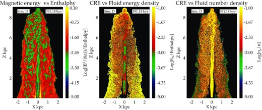
Figures demonstrating fractional energies between different components as a measure of equipartition. Left: Ratio of the magnetic field energy density to the relativistic fluid enthalpy. Middle: Ratio of the CRE energy density to the fluid enthalpy. Right: Ratio of the CRE number density to the fluid number density. See text in Section 5.7 for details.
The middle panel of Fig. 18 shows the CRE energy deposited on the computational grid using the ‘Cloud-in-Cell’ (CIC) approach of weighting, as described in section 3.3 of Mignone et al. (2018). Inside the jet axis, the particle energy is enhanced at certain locations (in red) with lower energy islands following them. These regions of enhanced particle energy correspond to recollimation shocks inside the jet beam where the particles are energized and accelerated. In the cocoon, the particle energy has a more homogeneous distribution. The ratio of particle energy to enthalpy is larger at the edges of the cocoon, due to decline of the fluid pressure. The particle number density is highest inside the jet axis, and uniformly distributed inside the cocoon. The ratio of particle number density to the fluid is capped at 0.1 due to enforced choice of fN = 0.1 in equation (5) in the present simulations.
We have to caution that the results presented in this section have some limitations due to their dependence on the somewhat arbitrary choices of the two parameters fE and fN. However, the general qualitative trends shown in this section are expected to hold. Additionally, we do not account for the backreaction of the relativistic particle population on the fluid, although in some locations their energy density becomes comparable to the fluid enthalpy. Recent works (e.g. Bromberg & Levinson 2009; Bodo & Tavecchio 2018) have shown that radiative losses can affect the structure of flow in shocked regions. However, in our simulations, fluid enthalpy becomes comparable to the CRE energy density only at certain regions in the cocoon of unstable jets, which are not expected to harbour strong shocks. Hence, the lack of radiative losses in our simulations are not expected to strongly affect the flow dynamics and the qualitative results presented here. The effect of coupling radiative losses to the fluid equations, however, will be addressed in future works.
6 DISCUSSION AND SUMMARY
In this paper, we have presented 3D time-dependent numerical simulations of non-thermal CREs embedded in an ideal relativistic magnetohydrodynamic flow jets of typical length-scales ∼ 10 kpc. By exploring different jet conditions, we have focused on the impact of MHD instabilities not only on the overall jet morphological structure but also on the spatial distribution of the CREs along the jet beam and its backflow, and the corresponding impact on the CRE spectrum.
Our results aim at surpassing semi-analytical models, previously proposed to describe the evolution of the CRE spectrum in the cocoon backflow (viz. the KP, JP, and Tribble models, see Harwood et al. 2013, for a review). Indeed, the vast majority of these models rely on several simplistic assumptions for ease of computation, such as constant magnetic field in the cocoon and constant pitch angle (KP model; Pacholczyk 1970), or a constant magnetic field and isotropic pitch angle (JP model Jaffe & Perola 1973), or a magnetic field distribution evolving with time due to adiabatic expansion of the cocoon (Murgia et al. 1999) or a turbulent magnetic field distribution in the cocoon (Tribble 1991; Hardcastle 2013). However, a time-dependent scenario, such as the one explored here, is likely to create complex flow features where non-thermal electrons can experience multiple shock crossings with non-trivial geometries. Last but not least, the effect of fluid instability can considerably affect the magnetic field strength in localized regions of space.
We can summarize our primary results and their implications as follows:
Stable jets: Non-thermal electrons in stable jets show the expected trends (as in Fig. 3) of being first accelerated at recollimation shocks inside the jet axis and then the jet head, followed by settling motions in the backflow of the cocoon. This is similar to the classic CRE evolutionary models proposed in early works (Jaffe & Perola 1973) where the jet axis and hotspot are filled with young energized electrons and the cocoon has older cooler electrons.
Multiple shock encounter in unstable jets: CREs undergo repeated acceleration in unstable jets at shocks of varying strengths and magnetic field. This can leave an imprint on the slope and maximum energy of the spectra. Kink instabilities lead to bending of the jet head which cause complex shock structures with extended curved features. The CREs thus experience repeated acceleration events before entering the backflow. KH instabilities in low magnetic field jets produce internal turbulence and vortices. This causes the CREs to have complex motions while travelling along the main jet flow as they spiral in local vortices. Reaccelerations of electrons in turbulent cocoons of unstable jets, coupled with slower expansion speed, also result in excess build of CRE energy in the jet cocoons, as discussed in Section 5.7.
Several aspects of the above results, such as the complex shocks in the lobes and multiple shock crossings of particles in the backflow, are complimentary to recent findings from relativistic hydrodynamic simulations of large scale jets by Matthews et al. (2019). Such shocks have been proposed to be conducive to the production of Ultra High Energy Cosmic Rays (UHCER), as shown in Bell et al. (2019). Qualitative agreements between the nature of evolution of the shock structures between our results, though on different physical scales, lends further support to the possibility of accelerating cosmic rays in shocks of extragalactic jets.
Turbulent jets thus create a distinct population of freshly accelerated electrons which have undergone several encounters with internal shocks. Such CREs are markedly absent in stable jets, indicating that creation of a separate energetic population of electrons is inherently related to the local dynamics of the fluid and the resultant shock acceleration. Presence of a secondary population has been often invoked to explain the excess observed emission at high-energy bands of some jets, modelled as synchrotron emission from an energized electron population with γe ≳ 107 (Atoyan & Dermer 2004; Kataoka & Stawarz 2005; Hardcastle 2006; Jester et al. 2006; Meyer et al. 2015; Migliori et al. 2020). Such a scenario has also been proposed by Borse et al. (2021) in local simulations of particle accelerations of a section of a non-relativistic jet. In this work, we demonstrate that reacceleration at internal shocks in the cocoon and the jet can indeed create a distinct secondary population of energized electrons as theorized in the above works, and that this is more pronounced in jets prone to MHD instabilities.
An important implication of CREs being energized in the cocoon is that the mean spectral index of the electrons and hence also the synchrotron spectrum is expected to become shallower. This is similar to the ‘continuous injection’ model used to describe spectrum of observed sources (Murgia et al. 1999; Brienza et al. 2018) with shallow radio spectral slopes, indicative of fresh injection of accelerated electrons. This will be further addressed in a forthcoming work, where we will present the observable synchrotron emission expected from our simulations (Paper III, Mukherjee et al., in preparation).
Mixing of CRE population: In the same simulation, CREs with different trajectories can experience very different fluid conditions, which affect their spectrum, as shown for particles P2 and P3 of simulation B in Section 5.2. CREs can be accelerated to high energies both if they cross strong shocks or if they pass through regions of low magnetic field where slower synchrotron cooling time-scales result in more efficient acceleration. Thus at a given height, there will be mixing of different population of electrons, with different evolutionary history. The distribution of CRE ages in the cocoon since their injection in the simulation is well described by approximate analytical model of backflow presented in Section 5.5.
Impact of shock encounters on CRE spectrum: The spectrum of a CRE that has undergone multiple shock crossings is a piece-wise power law (see Section 5.6.1). The cooling spectrum, however, finally attains the shape of a power law with exponential cut-off, with the slope at lower energies being determined by its strongest shock encounter. Since CREs with different shock histories lie at similar locations, spatially averaged spectrum of a region will have imprints from different cooling populations. This can cause the spectrum to have complex shapes that are best modelled by superposition of different cut-off power laws due to the different CREs (e.g. Fig. 16). The resultant envelope shows a curved spectrum at the higher energies. Such results have also been hinted in earlier works such Micono et al. (1999) and Meli & Biermann (2013), which have modelled multiple shock encounters of electrons at different recollimation shocks inside the jet axis. Our results show that this will be expected also in the cocoons of turbulent jets. Observed curvature in radio spectrum of some sources have been attributed to intrinsic property of the electron distribution itself by some recent papers, such as Duffy & Blundell (2012) and Nyland et al. (2020). Such curvature at higher energies of the spectrum naturally arises in our simulations due to multiple shocked populations.
In the current work, we have focused on presenting the results of the dynamics and spectral evolution of non-thermal electrons injected with the jet and the impact of MHD instabilities. In future papers, we will present the implications of these results on the observable non-thermal emission arising from processes such as Synchrotron and inverse-Compton; and how differences in jet dynamics and internal fluid properties affect such emission processes.
ACKNOWLEDGEMENTS
We thank the referee for their constructive comments which helped to improve the clarity of the paper. We acknowledge support by CINECA through the Italian Super Computing Resource Allocation (ISCRA) scheme and by the Accordo Quadro INAF-CINECA 2017 for the availability of high- performance computing resources. The authors acknowledge support from the PRIN-MIUR project Multi-scale Simulations of High-Energy Astrophysical Plasmas (Prot. 2015L5EE2Y). Bhargav Vaidya would like to acknowledge the support provided from Max Planck Society (MPG) in establishing Max Planck Partner Group at IIT Indore.
DATA AVAILABILITY
The derived data generated in this research will be shared on reasonable request to the corresponding author.
Footnotes
A parallel shock has its normal close to the down-stream magnetic field. The shock normal and downstream magnetic field are at large angles for perpendicular shocks.
It is to be noted that as a particle exits a shock into the downstream region, there may exist other particles inside the computational cell which may have been advected there without passing through a shock, or are remnants of a previous shock exit.
Depending on the orientation of the downstream magnetic field with respect to the shock normal, a shock is considered quasi-perpendicular if cos θB2 ≤ 1/η (Takamoto & Kirk 2015). In this work, we assume a shock with θB2 > 45° as perpendicular. This sets the assumed value of η for the limit θB2 = 45°.
REFERENCES
APPENDIX: A SUMMARY OF THE METHOD TO EVOLVE CRES IN SIMULATIONS
A1 Phase-space evolution of a CRE not in a shock
The CREs are evolved both in space and energy following the 6D Boltzmann transport equation (Webb 1989; Mimica et al. 2009; Vaidya et al. 2018) after ignoring the effect of spatial diffusion, shear and viscous energy exchanges, Fermi second-order processes, and non-inertial energy changes as outlined in Section 2 of Vaidya et al. (2018, hereafter BV18). The number of particles per unit volume in the energy range (E, E + dE) is given by N(E, t)dE. Each CRE macro-particle represents an ensemble of non-thermal electrons with an energy distribution defined by a spectrum, which in our work is discretized into finite logarithmically placed energy bins. For this work, the spectra have been defined on 100 bins. The spatial location (xp) of a macro-particle is updated by solving dxp/dt = v(xp), where v(xp) is the velocity of the fluid interpolated on to the location of the CRE macro-particle.
τ is the proper time that is related to the time in observer frame as dτ = dt/γ, γ being the bulk Lorentz factor of the particle. σT is the Thompson scattering cross-section, β is the velocity of the particle normalized to the speed of light (c), me is electron mass, B is the magnetic field interpolated at the location of the particle, arad is the radiation constant, and T0 = 2.728 K is the CMB temperature at z = 0.
Note that equation (A1) implies that the number density of CRE in the energy bin remains conserved. However, the edges of the energy bins evolve according to equation (A2). Thus coupled together, equations (A1) and (A2) describe the evolution of CREs with an averaged number density of Np(E0, 0) in an energy bin of range (E0, E0 + dE0) at τ = 0, as they evolve to time τ. In practise, the spectrum of a CRE is updated at each time-step by evolving the energy bins of the discretized spectrum following equation (A2) while preserving the value of Np(E0, 0) for the energy bin (Vaidya et al. 2018; Huber et al. 2021).
A2 Spectral update at shocks
A2.1 Identifying entry and exit of shocks by CREs
The above criteria, which depends on the history of the pressure change experienced by the particle, coupled with that in equation (A5) are together used to identify if a CRE has successfully entered and exited a shock, and is due for a shock-update based on implementation of diffusive shock acceleration outlined in the next section.
A2.2 Implementation of DSA
The two most important parameters of equation (A9) are the strength of the magnetic field (B) and the shock compression ratio (r), defined in equation (A7). Thus a CRE can be accelerated to high energies if it passes through a strong shock with high compression ratio r and/or low magnetic field, resulting in increased synchrotron cooling time-scales, and thus more efficient acceleration. Thus both at the jet head where the shock strength is high, and as well as in a turbulent cocoon where weak shocks may lie in regions of relatively lower magnetic field strengths, CREs can be accelerated to high energies.
A3 Interpolating a CRE spectrum
Spectrum of a CRE is often needed to be interpolated on to a new energy array, such as while performing the integral to convolve the spectra at a shock update described in Section 2.1.2, or while adding spectra of many different CRE to get a total spectrum from an area, as done in Section 5.6.2. While interpolating, first a new logarithmically spaced energy array is created with its end points set appropriately. For example while adding two spectra, the extrema are set to the lowest and the highest of the two spectra, respectively. For performing the convolution in Section 2.1.2, the lowest energy is unchanged, while the highest energy edge defined from the shock acceleration prescription using equation (A8).
