


ABSTRACT
The distribution of ionized hydrogen during the epoch of reionization (EoR) has a complex morphology. We propose to measure the 3D topology of ionized regions using the Betti numbers. These quantify the topology using the number of components, tunnels, and cavities in any given field. Based on the results for a set of reionization simulations we find that the Betti numbers of the ionization field show a characteristic evolution during reionization, with peaks in the different Betti numbers characterizing different stages of the process. The shapes of their evolutionary curves can be fitted with simple analytical functions. We also observe that the evolution of the Betti numbers shows a clear connection with the percolation of the ionized and neutral regions and differs between different reionization scenarios. Through these properties, the Betti numbers provide a more useful description of the topology than the widely studied Euler characteristic or genus. The morphology of the ionization field will be imprinted on the redshifted 21-cm signal from the EoR. We construct mock image cubes using the properties of the low-frequency element of the future Square Kilometre Array and show that we can extract the Betti numbers from such data sets if an observation time of 1000 h is used. Even for a much shorter observation time of 100 h, some topological information can be extracted for the middle and later stages of reionization. We also find that the topological information extracted from the mock 21-cm observations can put constraints on reionization models.
1 INTRODUCTION
The 21-cm signal produced by the hyperfine transition of neutral hydrogen is one of the most promising signals for probing the period from the history of our Universe when it transitioned from a cold and neutral state to a hot and ionized state (e.g. Furlanetto, Oh & Briggs 2006; Morales & Wyithe 2010; Zaroubi 2013). This transition period is known as the epoch of reionization (EoR), and ended around redshift z ≈ 5.5–6 (Keating et al. 2019; Kulkarni et al. 2019; Nasir & D’Aloisio 2020). The 21-cm signal produced during EoR will be redshifted and found at the low frequency end of the radio band. It traces the distribution of neutral hydrogen gas present in the intergalactic medium (IGM). Observing this signal will therefore shed light not only on the progress of reionization but also on a range of other issues such as the formation of first compact structures (e.g. Barkana 2016).
The global signal experiment, Experiment to Detect the Global EoR Signature (EDGES; Bowman & Rogers 2010), has claimed a detection of the sky averaged 21-cm signal from z ≈ 17 (Bowman et al. 2018). This detection is debated as its nature questions our current understanding of the early Universe (e.g. Hills et al. 2018; Singh & Subrahmanyan 2019). See Tashiro, Kadota & Silk (2014), Barkana (2018), Fialkov, Barkana & Cohen (2018), Muñoz & Loeb (2018), Feng & Holder (2018), and Fialkov & Barkana (2019) for few possible theories that can explain the Bowman et al. (2018) observation. Other global experiments, such as the Large-aperture Experiment to Detect the Dark Age (LEDA; Price et al. 2018) the Dark Ages Radio Explorer (DARE; Burns et al. 2017) and SARAS2 (Singh et al. 2017) are also trying to detect the global 21-cm signal. As we wait for an independent experiment to confirm the Bowman et al. (2018) observation, we will assume the standard cosmology in this study.
There also exists numerous efforts to detect the fluctuations in the signal using interferometric radio telescopes, such as the Low Frequency Array (LOFAR; e.g. van Haarlem et al. 2013), the Murchison Widefield Array (MWA; e.g. Wayth et al. 2018), and Hydrogen Epoch of Reionization Array (HERA; e.g. Deboer et al. 2017). Even though the fluctuations have not been detected, upper limits have been placed on the 21-cm power spectrum (e.g. Mertens et al. 2020; Trott et al. 2020) that have started to put constraints on the reionization process (e.g. Ghara et al. 2020, 2021; Greig et al. 2020a, b; Mondal et al. 2020). In the near future, the low frequency element of the Square Kilometre Array (SKA-Low; e.g. Mellema et al. 2013; Koopmans et al. 2015) will start observing the 21-cm signal produced during the EoR. SKA-Low is expected to be sensitive enough to not only detect the 21-cm power spectrum but also to produce images (e.g. Mellema et al. 2015; Giri 2019).
The 21-cm signal produced during EoR is highly non-Gaussian and therefore cannot be completely characterized by the 21-cm power spectrum (e.g. Majumdar et al. 2018). Therefore, we need to explore other summary statistics that are sensitive to the non-Gaussian information contained in the signal. Examples of such summary statistics that have been studied previously are the bispectrum (Majumdar et al. 2018; Watkinson et al. 2019), the position-dependent power spectrum (Giri et al. 2019b), size distributions (Kakiichi et al. 2017; Giri et al. 2018a, 2019a; Busch et al. 2020), and fractal dimensions (Bandyopadhyay, Choudhury & Seshadri 2017).
Yet another probe of the non-Gaussian information in the 21-cm signal is a summary statistics that describes the topology of the signal. This topology is quite sensitive to the properties of ioninzing sources (e.g. Hutter et al. 2021). Already Gnedin (2000) used the topology of the H ii (or ionized) regions to heuristically describe the EoR to consist of three stages, namely the preoverlap, overlap, and post-overlap stage. Subsequent studies quantified the topology using the genus g or its equivalent the Euler characteristic χ (χ = 2 − 2g) of the neutral hydrogen distribution (e.g. Gleser et al. 2006; Lee et al. 2008) or the ionization fraction field (Friedrich et al. 2011). These works could build on the extensive literature about the use of χ (or g) on the large-scale structure (e.g. Gott, Dickinson & Melott 1986; Gott et al. 1992; Matsubara 1994; Matsubara & Yokoyama 1996; Schmalzing & Buchert 1997; Park, Kim & Gott 2005).
The Euler characteristic is also equivalent to the third of the Minkowski functionals V3 and some works have considered the full set of these topological quantities (V0–V3; Friedrich et al. 2011; Yoshiura et al. 2017; Chen et al. 2019). Based on the evolution of the Minkowski functionals the latter study proposed a five stage description of the reionization process.
During reionization the distribution of ionized bubbles will imprint its topology on the observable 21-cm signal. Therefore, we will also discuss the prospects of measuring the Betti numbers of 3D structures in the upcoming 21-cm observations with SKA-Low, considering both resolution and noise effects. As far as we know there exists very few work that considered the Betti numbers in the context of reionization. Elbers & Van De Weygaert (2019) studied the Betti numbers in heuristic models of reionization that they called the H ii bubble network. Kapahtia et al. (2018, 2021) and Kapahtia, Chingangbam & Appleby (2019) only studied the Betti numbers for 2D 21-cm images. However, reionization is a 3D process and SKA-Low will produce 3D data cubes consisting of images at a range of frequencies. We will therefore study the three Betti numbers associated with the 3D topology.
There exists even more metrics to study the topology, such as the persistence homology (e.g. Zomorodian & Carlsson 2005; Edelsbrunner & Harer 2008) that is gaining attention in cosmology (e.g. van de Weygaert et al. 2010, 2011; Sousbie 2011; Sousbie, Pichon & Kawahara 2011; Pranav et al. 2017; Makarenko et al. 2018; Wilding et al. 2020). In persistence homology, the evolution of each κ-dimensional holes in the analysed field is tracked. Elbers & Van De Weygaert (2019) have used persistence homology to study the H ii bubble network. We defer the exploration of persistence homology of 21-cm data sets to future studies.
The paper is structured as follows. In the next section, we describe the topological concepts used throughout the paper. Section 3 explains explains our large-scale reionization simulations and the methods used to construct the 21-cm signal from simulation outputs. In Sections 4 and 5, we discuss the properties and evolution of the Betti numbers of the ionization and 21-cm signal fields, respectively. We discuss the detectability of the Betti numbers in 21-cm observations of upcoming radio telescopes in Section 6. In the final section, we summarize our findings.
2 TOPOLOGICAL MEASURES
In this section, we describe the methods we use to measure the topology of our data. In Section 2.1, we explain the metric we will use to quantify the topology of any field. The fields we analyse in this study are given in form of digital data. Therefore, we define an estimator for measuring the topology of digital data in Section 2.2.
2.1 Betti numbers
In this study, we quantify the topology of structures in our field with the Betti numbers (βκ) that are topological invariant quantities (Betti 1870). This means they remain unchanged under transformations, such as translation, rotation, and deformation. βκ is defined as the number of κ-dimensional holes in the structure we analyse. Our data sets are 3D and therefore their topology can be defined with three Betti numbers where each have a simple and intuitive meaning. The zeroth Betti number (β0), first Betti number (β1), and second Betti number (β2) probe the number of isolated objects, tunnels, and cavities, respectively.
In its simplest form, the reionization process can be pictured as a network formed by bubbles of ionized hydrogen gas. In Fig. 1 we show examples of structures formed by spherical bubbles. The left-hand and right-hand panels show projections of 3D data sets containing one and five spherical bubbles, respectively. As they both consist of a single connected structure, both data sets have β0 = 1. The data set in the left-hand panel has no tunnel, hence its β1 = 0. The five bubbles in the right-hand panel form a torus, which contains a tunnel, giving β1 = 1. The projection does not reveal the inner structure of the spheres. If we assume that the single sphere in the left-hand panel has a hollow centre, then this single cavity will give β2 = 1. If we assume that the spheres in the right-hand panel are all filled, this gives β2 = 0.
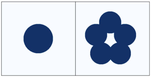
Projection of two different configurations of spheres where the one of the left is hollow. These configurations have Betti numbers βκ = (1, 0, 1) (left) and βκ = (1, 1, 0) (right), giving Euler characteristics χ = 2 and χ = 0, respectively.
2.2 Estimators for digital data
All the fields that we work with in this study are digital data, which is a discrete, discontinuous representation of a given field. In order to capture the topology of the structures in our field, we need to decompose the structures into well-defined geometrical components in such a way that the topological properties of the structure are retained. We achieve this by constructing a cubical complex (e.g. Kaczynski, Mischaikow & Mrozek 2004; Wagner, Chen & Vuçini 2012), which is composed of points, line segments, squares, and cubes, for any given field. We refer the readers to Wagner et al. (2012) and Giri et al. (2019a) for more information about our method to construct and store our cubical complex.
2.2.1 Betti numbers
We follow the method described in Gonzalez-Lorenzo et al. (2016) to estimate the Betti numbers. Each isolated object is a group of connected pixels in our data set. We use the connected-component labelling module in scikit-image package1 (van der Walt et al. 2014). We refer inquisitive readers to Fiorio & Gustedt (1996) and Wu, Otoo & Shoshani (2005) for the algorithm used to label all the connected regions. This method needs less computation time compared to the classical Hoshen–Kopelman algorithm (Hoshen & Kopelman 1976). It is similar to the friends-of-friend algorithm used to find clusters in N-body simulations (e.g. Press & Davis 1982; Davis et al. 1985). The number of regions labelled gives the value of β0.
From the Alexander duality of any topological complex of three dimensions, we can find the β2 by estimating the β0 of the complementary field of the data set (e.g. Hatcher 2002; Gonzalez-Lorenzo et al. 2016). The remaining first Betti number β1 is not calculated directly, but derived from the Euler characteristics (χ) of the data set (as described in Section 2.2.2) according to β1 = β0 + β2 − χ. This method of calculating the β1 was introduced by Gonzalez-Lorenzo et al. (2016). We have tested our estimator on a Gaussian random field (GRF). The results are presented in Appendix A.
2.2.2 Euler characteristics
3 SIMULATION OF 21 CM SIGNAL
To test the usefulness of the Betti numbers we make use of simulated data. This section describes our methodology for simulating reionization and the 21-cm signal. Section 3.1 describes the large-scale reionization simulations we use and Section 3.2 outlines how we calculate the observable 21-cm signal from them. Finally we explain how we include telescope effects, such as the limited angular resolution and telescope noise in Section 3.3.
3.1 Reionization simulations
We use two different types of reionization simulations for our study, fully numerical radiative transfer simulations, and so-called semi-numerical simulations that rely on sophisticated form of photon counting.
3.1.1 Fully numerical simulations
The fully numerical simulations use two steps. We first simulate the evolution of the matter distribution using the N-body code CUBEP3M (Harnois-Déraps et al. 2013). The N-body simulation is run in a cosmological volume of 714 comoving Mpc (cMpc) with 69123 particles. We use such a large cosmological volume as they are important to capture the large-scale fluctuations (Giri et al. 2019b; Ghara et al. 2020) and the large-scale topological structure (Giri et al. 2019a) and are also a match to the Field of View of SKA-Low. See Iliev et al. (2014) for a discussion about the importance of the size of cosmological volumes for reionization simulations. Our N-body simulation run outputs snapshots at each 11.5 Myr. We obtain the density field by assigning mass to a cubic grid with 300 cells along each direction by smoothing with a smooth-particle-hydrodynamics kernel (Monaghan 1992; Iliev et al. 2014). The cosmological parameters used here are Ωm = 0.27, Ωk = 0, Ωb = 0.044, h = 0.7, ns = 0.96, and σ8 = 0.8. These values are consistent with the results from Wilkinson Microwave Anisotropy Probe (WMAP; Komatsu et al. 2011) and Planck (Planck Collaboration 2016, 2018) collaborations.
To simulate the state of gas in the intergalactic medium, we next post-process the snapshots from CUBEP3M with the fully numerical radiative transfer code C2-RAY (Mellema et al. 2006a). C2RAY employs the short characteristics ray tracing method to solve the radiative transfer equation (Raga et al. 1999; Lim & Mellema 2003). The ray-tracing is performed up to a comoving distance of 71 Mpc from each source. This limit is meant to approximate the effect of the presence of optically thick absorbers in the IGM that are unresolved in our N-body simulation. This value is consistent with the measurement of the mean free path by Songaila & Cowie (2010). For more details about the simulations we refer the reader to Iliev et al. (2006), Mellema et al. (2006b), and Dixon et al. (2016).
In this work, we have run two scenarios (FN1 and FN2) using the methods described above. FN1 and FN2 use ζ values of 50 and 40, respectively. We show the history of these reionization scenarios in Fig. 2. As the sources are less efficient in FN2 compared to the FN1 scenario, reionization is delayed in the latter. The values of the source parameters are listed in Table 1. The Thompson scattering optical depth τ calculated from these simulations are within the 95 per cent credible interval of the constraints from Planck Collaboration (2018). The estimated τ are also given in Table 1.
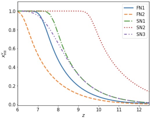
The volume weighted average ionization fraction of our reionization simulations varying over the redshifts.
Reionization simulation parameters of various source models. We give the ionizing source parameters that are ionizing efficiency (ζ), minimum mass (Mmin), and mean free path of ionizing photons (Rmfp). The Thompson scattering optical depth (τ) derived from each simulations are also given here.
| Label | Code | Box size (Mpc) | Mesh | ζ | Mmin(M⊙) | Rmfp (Mpc) | τ |
|---|---|---|---|---|---|---|---|
| FN1 | CUBEP3M + C2RAY | 714 | 3003 | 50 | 109 | 71 | 0.058 |
| FN2 | CUBEP3M + C2RAY | 714 | 3003 | 40 | 109 | 71 | 0.050 |
| SN1 | 21cmfast | 714 | 3003 | 50 | 109 | 71 | 0.064 |
| SN2 | 21cmfast | 714 | 3003 | 50 | 108 | 71 | 0.084 |
| SN3 | 21cmfast | 714 | 3003 | 50 | 109 | 20 | 0.062 |
3.1.2 Semi-numerical simulations
We have run three semi-numerical reionization scenarios (SN1, SN2, and SN3) by varying the source and sink parameters in 21cmfast. The values of the parameters are given in Table 1. We also show the reionzation history of these models in Fig. 2. Even though scenario SN1 has the same parameters as FN1, their reionization histories are not identical. This is because SN1 does not explicitly include the photon losses due to recombinations whereas FN1 does. In 21cmfast these losses are assumed to be accounted for in the value of ζ [see for e.g. equation (2) in Greig & Mesinger (2015)].
3.2 Redshifted 21 cm signal
Here we will work with the assumption of high-spin temperature Ts ≫ TCMB. During the EoR this is a reasonable assumption as even relatively low levels of X-ray radiation can raise the gas temperature above the CMB temperature (e.g. Pritchard & Furlanetto 2007; Pritchard & Loeb 2012). In the high-spin temperature limit, δTb is independent of Ts.
We construct the 21-cm signal at a given redshift z from equation (6) using the corresponding 3D neutral fraction and matter density cubes from the C2-RAY and CUBEP3M simulations. Each of these 3D data sets represents the characteristics of the signal at the corresponding redshift z and therefore called coeval cubes (CCs). We transform these CCs into image cubes by assuming one of the axes to be the frequency axis and the other two position in the sky. This procedure implies that we neglect the two line-of-sight effects: redshift space distortions (RSD; see e.g. Jensen et al. 2013) and the light-cone (LC) effect (see e.g. Datta et al. 2012) that would introduce minor distortions along the line of sight. We use our publicly available analysis code, tools21cm2 (Giri, Mellema & Jensen 2020a), to simulate the redshifted 21-cm signal cubes.
3.3 Mock SKA-Low observation
In this section, we explain our methods for constructing mock observation with SKA-Low.
3.3.1 Limited resolution
Apart from the simulation resolution, we will also be limited by the resolution of the telescope. As SKA-Low is an interferometry based radio telescope, it observes the sky in so-called uv space that corresponds to the Fourier transform of the sky. We refer the readers to Rohlfs & Wilson (2013) for details about radio telescope observations.
An interferometric radio telescope also has a smallest baseline that sets the largest scales that it can image. To implement this effect, we subtract its average value from each slice of the 21-cm signal data set along the frequency (or redshift) axis. This effect means that interferometric images lack absolute calibration of the signal. Finally, to attain isotropic resolution in our data set we convolve the signal along the frequency axis with a tophat filter of the same physical width as the Gaussian beam. For z = 8 this gives Δν ≈ 0.5 MHz.
3.3.2 System noise
The 21-cm observations with SKA-Low will also be prone to instrumental noise. In order to simulate this noise, we follow the approach in Ghara et al. (2017) and Giri, Mellema & Ghara (2018b). We model the effects using the currently available configuration3 of the first phase of SKA-Low that has 512 antennae stations each with a diameter of 35 m. We present the telescope parameters that we use in this study in Table 2.
The parameters used in this study to model the telescope properties.
| Parameters | Values |
|---|---|
| System temperature (Tsys) | |$60 (\frac{\nu }{300\mathrm{MHz}})^{-2.55}$| K |
| Effective collecting area (AD) | 962 m2 |
| Critical frequency (νc) | 110 MHz |
| Declination | −30° |
| Observation hour per day | 6 h |
| Signal integration time | 10 s |
| Parameters | Values |
|---|---|
| System temperature (Tsys) | |$60 (\frac{\nu }{300\mathrm{MHz}})^{-2.55}$| K |
| Effective collecting area (AD) | 962 m2 |
| Critical frequency (νc) | 110 MHz |
| Declination | −30° |
| Observation hour per day | 6 h |
| Signal integration time | 10 s |
We explore two observation time (tobs). One is an optimistic case of tobs = 1000 h and other is a pessimistic case of tobs = 100 h. At simulation resolution, the system noise at 1000 and 100 h will be very high. As the this noise is uncorrelated while the signal is correlated, the signal-to-noise ratio (SNR) will go up when the resolution is decreased. As discussed earlier, SKA-Low will have a limited resolution defined by the maximum baseline. Previous studies have shown that we can get interesting image data with 1000 h observation at a resolution corresponding to B = 2 km (e.g. Mellema et al. 2015; Ghara et al. 2017; Giri et al. 2018b, 2019a). However the SNR will be much lower for a 100 h observation at the same resolution. To achieve a similar SNR, we reduce the resolution by a factor of 2 for the 100 h mock observations.
We would like to note that the noise model we use assumes perfect calibration. In reality it is not always possible to reach this theoretical noise level. Therefore, to achieve the same SNR values as in our example with the real SKA-Low might require longer observation times or use of a lower resolution.
4 BETTI NUMBERS OF IONIZATION FIELD
The formation, merger, and evolution of ionized bubbles during reionization results in a complex morphology of H ii regions. In this section we investigate the Betti numbers estimated from the ionization field in our simulations.
4.1 Evolution during reionization
Fig. 3 shows the evolution of Betti numbers estimated from the ionization field of our FN1 simulations by defining structures using a threshold of |$x_\mathrm{H\, \rm {ii}}=0.5$|. These Betti numbers trace the evolution topology of H ii regions during reionization. Here and in the remainder of this paper we plot the evolution of the Betti numbers against the fraction of our simulation volume that has been ionized, rather than time or redshift. Using the ionized volume fraction |$x_\mathrm{H\, \rm {ii}}^\mathrm{V}$| connects the evolution of the Betti numbers to the different stages of reionization and also makes it easier to compare the results of different reionization scenarios in which reionization may have evolved differently.
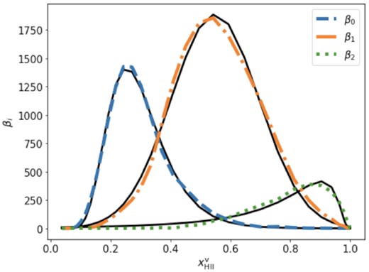
Evolution of the Betti numbers estimated from the |$x_\mathrm{H\, \rm {ii}}$| field of the FN1 simulation. The black solid lines are the fits to the curves. See text for a description of these fits and Table 3 for the fit parameters.
When reionization starts we see an increase in β0. This increase in β0 is due to the appearance of ionized bubbles around the sources emitting ionizing photons. As time passes, more sources form and ionize the hydrogen gas in the IGM around them. In the initial stages of reionization we not only see appearance of new ionized bubbles but also overlap of bubbles. A comparison between the value of β0 and the number of sources shows that such overlap occurs right from the start of reionization. The total number of bubbles will decrease when multiple ionized bubbles overlap. When the rate by which H ii regions start to overlap becomes larger than the formation rate of new isolated ionized bubbles, the value of β0 will start to decrease. In our model, we observe this turn-around at |$x^\mathrm{v}_\mathrm{H\, \rm {ii}}\approx 0.2$|. The value of β0 keeps decreasing as reionization proceeds and converges to unity at around |$x^\mathrm{v}_\mathrm{H\, \rm {ii}}\approx 0.7$|.
At |$x^\mathrm{v}_\mathrm{H\, \rm {ii}}\approx 0.1$|, β1 starts to increase. β1 measures the number of tunnels and these tunnels can be formed by overlapping bubbles (see Section 2.1 for a simple example). Therefore, the growth of β1 is a sign of substantial bubble overlap modulating the topology of the ionization field. As reionization progresses, the number of tunnels increase until it reaches a maximum value beyond which β1 starts to decrease. In the FN1 simulation this peak is reached around |$x^\mathrm{v}_\mathrm{H\, \rm {ii}}\approx 0.55$|. Unlike β0, the value of β1 remains much larger than 1 until the end of reionization.
Cavities inside H ii regions start forming during the middle stages of reionization, as indicated by the slow rise of β2, starting around |$x^\mathrm{v}_\mathrm{H\, \rm {ii}}\approx 0.2$|. We can visualize these cavities as isolated neutral regions. As reionization progresses initially large connected neutral regions breakup and form multiple isolated neutral regions. The value of β2 attains a maximum around |$x^\mathrm{v}_\mathrm{H\, \rm {ii}}\approx 0.9$| after which it falls to zero once reionization completes. In any inside-out reionization scenario such as FN1, these later isolated neutral regions trace the cosmic voids. Giri et al. (2019a) noted that the number of isolated neutral regions in the later stages of reionization are relatively rare compared to the number of isolated ionized regions at the start of reionization. This is confirmed by comparing the maximum values of the β0 and β2 curves, which shows that the latter is about 3.5 times lower.
From the three curves we obtain three clear maxima, as well as the crossing points between β0 and β1 as well as between β1 and β2. As β1 enters the calculation of the Euler characteristic χ with a different sign than β0 and β2, the above evolutionary patterns cannot be distinguished when considering χ. It is for example impossible to separate the early rise of the number of tunnels and the decrease of the number of isolated regions due to overlap. At |$x^\mathrm{v}_\mathrm{H\, \rm {ii}}\approx 0.35$| β0 ≈ β1. However the small positive contribution from β2 at that time will push the location of χ = 0 to a slightly later stage.
4.2 Connection between Betti numbers and percolation
These crossing points of Betti curves appear to be connected to the formation of the percolation clusters. Furlanetto & Oh (2016) showed that a large network of overlapping ionized bubbles spanning the entire simulation volume forms during the early stages of reionization. This network is known as the percolation cluster. A similar percolation event4 takes place towards the end of reionization when the last network of neutral regions spanning the entire volume disappears. As pointed out by Furlanetto & Oh (2016) this type of percolation behaviour is a hallmark of phase transitions.
Fig. 4 shows the percolation curves, i.e. the volume fraction of H ii regions contained in the percolation cluster, for all our simulations. Here we focus on the percolation curve of the FN1 scenario; the percolation curves of other scenarios are discussed in Section 4.5. We see that the appearance of the percolation cluster coincides with the time when β1 surpasses β0. Likewise we find that the disappearance of the neutral percolation cluster coincides with the time when β1 ≈ β2. It was recently proposed by Santos et al. (2019) and Bobrowski & Skraba (2020) that such a connection between Betti numbers and percolation may be universal.
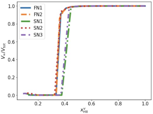
Percolation curves for the ionized percolation cluster. The number on the ordinate, V∞/Vtot, is the fraction of the total ionized volume contained in the percolation cluster. The different curves show the evolution of this quantity for our five different reionization scenarios.
4.3 Parametrization of the evolution of Betti numbers
The values of parameters when we model the Betti numbers using equations (10), (11), and (12). The fit parameters for |$x_\mathrm{H\, \rm {ii}}$| are Betti number curves estimated from the field at simulation resolution. The fit parameters for δTb are Betti number curves estimated from the mock SKA-Low 21-cm images. We give the fit parameters corresponding to mock observations at tobs = 1000 h and B = 2 km. The fit parameters given in brackets correspond to mock observations at tobs = 100 h and B = 1 km.
| Fit | |$\pmb {x_\mathrm{H\, \rm {ii}}}$| | |$\pmb {\delta T_\mathrm{b}}$| | |||||
|---|---|---|---|---|---|---|---|
| Models | Parameters | β0 | β1 | β2 | β0 | β1 | β2 |
| FN1 | Ai | 1409 | 1886 | 415 | 50 (–) | 512 (443) | 92 (80) |
| μi | 0.25 | 0.55 | 0.10 | 0.27 (–) | 0.61 (0.61) | 0.04 (0.03) | |
| σi | 0.71 | 0.15 | 0.43 | 0.55 (–) | 0.16 (0.18) | 0.33 (0.34) | |
| FN2 | Ai | 1443 | 2092 | 476 | 156 (–) | 562 (500) | 90 (80) |
| μi | 0.27 | 0.55 | 0.11 | 0.29 (–) | 0.63 (0.62) | 0.04 (0.03) | |
| σi | 0.75 | 0.14 | 0.46 | 0.72 (–) | 0.15 (0.18) | 0.38 (0.36) | |
| SN1 | Ai | 1195 | 1652 | 112 | 161 (–) | 470 (371) | 43 (45) |
| μi | 0.21 | 0.56 | 0.06 | 0.24 (–) | 0.61 (0.63) | 0.03 (0.05) | |
| σi | 0.63 | 0.16 | 0.37 | 0.69 (–) | 0.16 (0.15) | 0.26 (0.45) | |
| SN2 | Ai | 1351 | 2168 | 223 | 66 (–) | 461 (342) | 43 (25) |
| μi | 0.25 | 0.56 | 0.08 | 0.31 (–) | 0.60 (0.64) | 0.02 (0.05) | |
| σi | 0.69 | 0.15 | 0.41 | 0.64 (–) | 0.19 (0.16) | 0.19 (0.25) | |
| SN3 | Ai | 1206 | 2048 | 800 | 138 (–) | 689 (688) | 130 (200) |
| μi | 0.21 | 0.55 | 0.09 | 0.24 (–) | 0.61 (0.67) | 0.03 (0.05) | |
| σi | 0.64 | 0.15 | 0.48 | 0.68 (–) | 0.16 (0.11) | 0.19 (0.45) |
The fact that simple functional forms can be used to describe the evolution of the Betti numbers for reionization is another advantage over the Euler characteristic for which no simple fit appears to exist.
4.4 Dependence on simulation resolution
The topology of H ii regions is sensitive to the resolution of our simulation volume. Friedrich et al. (2011) showed the impact of simulation resolution on the Euler characteristics. In this section, we study how the Betti numbers depend on the simulation resolution.
We show the Betti numbers curves estimated from the FN1 simulation volumes at different resolutions in Fig. 5. The solid curve represents the Betti numbers estimated from the data set at the intrinsic resolution of our simulation (Δx ≈ 2.4 Mpc). The dashed and dash–dotted lines represent their values estimated after four-cell and eight-cell smoothing, respectively. The four-cell and eight-cell smoothing approximately correspond to the resolution of SKA-Low observations at z ≈ 9 when maximum baselines of 2 and 1 km are used, respectively.
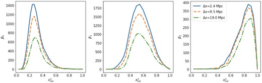
Evolution of the Betti numbers estimated from the |$x_\mathrm{H\, \rm {ii}}$| field of the FN1 simulation at various resolutions. The solid, dashed, and dash–dotted line-styles give Betti numbers estimated from data set at simulation resolution, four-cell smoothing, and eight-cell smoothing, respectively. The latter two approximately correspond to the resolution achieved by SKA-Low observations with a maximum baseline of 2 and 1 km, respectively, for redshift z ≈ 9.
When we fit these curves with the parametric form given in equations (10), (11), and (12), we find that the peak positions and widths of the curve do not change as the resolution degrades. The resolution only affects the amplitude parameter Ai for all the Betti numbers curve. This decrease in amplitude is expected as the number of features contained in the data set decreases when the resolution is degraded. The fact that the peak positions and widths are less affected adds to the attractiveness of the Betti numbers as topological quantities.
4.5 Comparing the topology of different reionization scenarios
In this section we compare the topology of various reionization models using the Betti numbers. The top panels of Fig. 6 show the Betti curves for our fully numerical simulations. The FN1 and FN2 simulations use source efficiencies ζ = 50 and 40, respectively. Therefore, reionization is delayed in FN2 (see Fig. 2). However, even though the reionization history is different the peak positions of the Betti curves are quite similar. The β0 gives the number of isolated ionized regions and at early times, this number will be proportional to the number of active ionizing sources and not the efficiency of those sources. Note, however, that β0 will not be exactly equal to the number of sources as some regions are formed by clustered sources. Fig. 2 shows that FN2 reaches a similar stage Δz ≈ 1 later than FN1. The number density of ionizing sources will not differ that much between those two epochs. Therefore, the β0 curves for both these models are quite similar. However, the topology does differ, as evidenced by the β1 and β2 curves. The FN2 simulation contains more tunnels during the middle stages of reionization and more cavities from about the middle until near the end of reionization. Using all the curves together, we can distinguish between these two models.
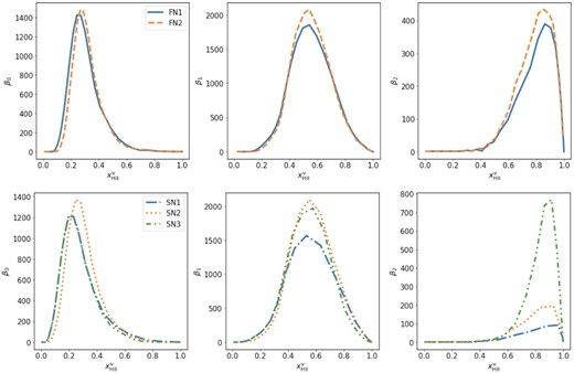
Evolution of the Betti numbers estimated from the |$x_\mathrm{H\, \rm {ii}}$| field of different simulations. The top and bottom panels show the Betti numbers for our fully numerical and semi-numerical simulation models, respectively.
To test the robustness of our conclusions, we also study the topology of reionization in a set of semi-numerical simulations. As semi-numerical simulations are fast, we can easily vary the simulation parameters and observe its impact on the Betti numbers. In the bottom panel of Fig. 6, we show the Betti numbers curves for our three semi-numerical simulations (see Table 1). SN1 and SN3 use the same Mmin value (|$10^9 \, \mathrm{M}_\odot$|) for dark matter haloes, which means that reionization is driven by the same source population. Therefore, the β0 curves for SN1 and SN3 overlap with each other. The Mmin used in SN2 is |$10^8 \, \mathrm{M}_\odot$|. As a result SN2 contains more ionizing sources compared to SN1 and SN3. We see the imprint of this on the β0 curve that reaches a higher amplitude for the SN2 simulation.
The SN1 and SN2 simulations assume Rmfp to be 71 Mpc where as SN3 simulation assumes it to be 20 Mpc. SN1 and SN3 otherwise have the same source parameters. Rmfp describes the largest distance ionizing photons can travel from a source. At the early times, the value of Rmfp does not have a significant impact on the topology as most H ii regions are smaller than Rmfp. However, once larger regions form during the middle and late stages of reionization, a smaller value for Rmfp will inhibit the growth of ionized regions. This will allow more tunnels to survive, as evidenced by the difference between the β1 curves of SN1 and SN3. The largest impact of Rmfp is associated with the final phases of reionization as can be seen from the β2 curves. The values are much higher for SN3, indicating that imposing a short mean free path leads to the formation of many more small neutral islands.
As pointed out in Section 4, the rise of β1 in simulation FN1 marks the appearance of the percolation cluster. The percolation curves for all our reionization models can be found in Fig. 4. We find that for all models, percolation happens roughly at the epoch when β1 crosses β0 confirming our hypotesis.
The Betti numbers curves from all our reionization models, both fully numerical and semi-numerical, show the characteristic forms defined in Section 4. We present the values of the fit parameters for all models in Table 3. We conclude that these fitting formulae equations (10), (11), and (12) provide a useful description of the evolution of Betti numbers in reionization simulations.
5 BETTI NUMBERS OF 21-CM SIGNAL
In this section we will study the evolution of Betti numbers estimated from the 21-cm signal (δTb). As explained in Section 3.2, this signal depends on neutral fraction |$\big (x_\mathrm{H\, \rm {i}}(\pmb {r}) = 1-x_\mathrm{H\, \rm {ii}}(\pmb {r}) \big)$|, density, and spin temperature fields (see equation 6). For our study we assume the Universe has been heated before reionization begins causing the spin temperature factor to saturate to 1 as (Ts ≫ TCMB). Even with this assumption, the δTb will still contain properties of both the ionization and density fields.
We first study the topology of structures by putting a threshold (|$\delta T^\mathrm{th}_\mathrm{b}$|) on the δTb field. We measure the topology of structures with pixel values below a given value of |$\delta T^\mathrm{th}_\mathrm{b}$|. In Fig. 7, we show colour plots of the Betti numbers estimated from the δTb field of the FN1 simulation against the values of |$\delta T^\mathrm{th}_\mathrm{b}$| (y-axis) and |$x^\mathrm{v}_\mathrm{H\, \rm {ii}}$| (x-axis). For high values of |$\delta T^\mathrm{th}_\mathrm{b}$|, the topology is mostly defined by the fluctuations in the density field. However the Betti numbers will not exactly trace the topology of the density field as reionization will reduce the signal in the (predominantly) dense regions. For low |$\delta T^\mathrm{th}_\mathrm{b}$| value, the structures trace the topology of ionization field. For |$\delta T^\mathrm{th}_\mathrm{b} \lesssim 10$| mK, the Betti numbers estimated from δTb fields are similar to that estimated from |$x_\mathrm{H\, \rm {ii}}$| field of FN1 simulation.
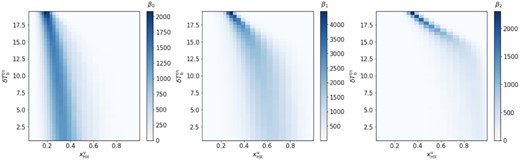
Contour plots of the values of β0 (left-hand panel), β1 (middle panel), and β2 (right-hand panel) of the δTb field from the FN1 simulation as a function of global ionization fraction |$x^\mathrm{v}_\mathrm{H\, \rm {ii}}$| and threshold value (|$\delta T^\mathrm{th}_\mathrm{b}$|).
For different reionization scenarios we will obtain different colour plots from the one shown in Fig. 7. However, it is difficult to compare scenarios with these plots as they will be affected by instrumental limitations such as lack of an absolute calibration of the signal, limited resolution, and noise. In the next section, we propose a method to explore the topological properties of reionization using mock 21-cm observations for the future SKA-Low telescope.
6 BETTI NUMBERS OF 21-CM IMAGES OBSERVED WITH RADIO TELESCOPE
As discussed in the previous section, the structures in the ionization field will be imprinted on the 21-cm signal. Therefore, we can study the morphology of H ii regions if we can identify these regions in 21-cm images. As the future SKA-Low has been designed to be able to produce such images (Mellema et al. 2015), we will consider mock SKA-Low observations in this section and study our ability to estimate the Betti numbers from such observations.
Identifying the ionized (or neutral) regions in 21-cm images is a non-trivial problem. Giri et al. (2018b) compared various methods taken from the field of image processing and found that the superpixel method works the best in identifying ionized (or neutral) regions in 21-cm images. In the superpixel method, connected pixels with similar properties are grouped together. These pixel groups are known as superpixels. We then construct the histogram from the mean intensity values of all the superpixels. From this histogram we find the threshold for the superpixels that classifies them into ionized and neutral superpixels. See Giri et al. (2018b) for a detailed description of the method. Note that the identification of the ionized regions at the same time yields an estimate for the fraction of the observed volume that is ionized, thus allowing to determine the Betti numbers as a function of ionized volume fraction rather than redshift.
In Section 6.1, we consider mock SKA-Low observations with infinite observation time as we want to first learn what we can achieve in this most optimal case with our method. In this situation, the 21-cm images will be free from noise and only be affected by the limited resolution and the lack of absolute calibration. In Section 6.2 we study the impact of telescope noise on our analysis strategy.
6.1 Limited resolution
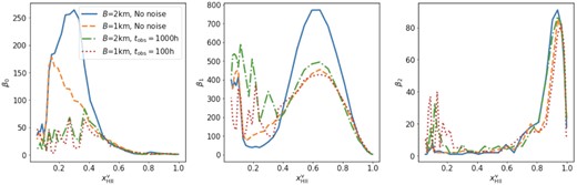
Fig. 8 shows the impact of SKA-Low resolution on the estimated Betti numbers. The solid and dashed lines represent the Betti numbers calculated from the |$x_\mathrm{H\, \rm {ii}}$| data sets degraded to a resolution corresponding to a maximum baseline (B) of 2 and 1 km, respectively. These curves differ slightly from the ones shown in Fig. 5 as the resolution corresponding to a certain value of B is redshift dependent. Even though the peak amplitude decreases as the resolution is degraded, the peak position of all the Betti number curves estimated from |$x_\mathrm{H\, \rm {ii}}$| does not change. This behaviour agrees with our findings in Section 4.4.
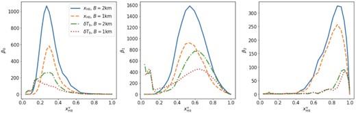
The solid and dashed (dash–dotted and dotted) represent Betti numbers curve estimated from the |$x_\mathrm{H\, \rm {ii}}$| (δTb) fields from simulation FN1 at resolutions corresponding to a maximum baseline B of 2 and 1 km, respectively.
The dash–dotted and dotted lines in Fig. 8 represent the Betti numbers estimated from the δTb fields at a resolution corresponding to B = 2 and 1 km, respectively. The peak position of β0 for the δTb field observed at B = 2 km matches the peak positions of the β0 curves derived from the |$x_\mathrm{H\, \rm {ii}}$| fields. However, for the lower resolution case of B = 1 km the β0 derived from the δTb fields attains its peak at a much earlier epoch. This is because the ionized regions are not very large at these early times and for the lower resolution the superpixel method struggles to separate the ionization and density fluctuations. This effect is in fact also present for the B = 2 km case where it causes the non-smooth increase of β0.
The middle panel of Fig. 8 shows that the β1 curves for δTb field are slightly biased towards larger |$x^\mathrm{v}_\mathrm{H\, \rm {ii}}$| compared to the ones for |$x_\mathrm{H\, \rm {ii}}$| field. We also observe that the peak amplitude of β1 curves for δTb field decreases and the width of the curve increases compared to the ones for |$x_\mathrm{H\, \rm {ii}}$| field. At early times (|$x^\mathrm{v}_\mathrm{H\, \rm {ii}}\lesssim 0.2$|), the β1 determined from |$x_\mathrm{H\, \rm {ii}}$| field is close to zero for all our reionization scenarios (see Section 4.5). However our method gives non-zero values for β1 determined from δTb field. This anomaly is again caused as the superpixel method struggles to separate ionization and density fluctuations during these early stages of reionization.
The right-most panel of Fig. 8 shows the β2 curves for δTb field. These curves are also slightly biased towards larger |$x^\mathrm{v}_\mathrm{H\, \rm {ii}}$| compared to the ones for |$x_\mathrm{H\, \rm {ii}}$| field. Even though the resolution corresponding to B = 1 km smooths away more features compared to B = 2 km, the superpixel method identifies similar number of neutral regions as these neutral regions are relatively large structures (Giri et al. 2019a). Therefore, the β2 curves for both resolution cases overlap with each other.
6.2 Telescope noise
The SKA-Low observations will contain instrumental noise, which we model using the method described in Section 3.3.2. Here we study the Betti numbers estimated from noisy 21-cm images. We consider two observation times, which are tobs = 1000 h and 100 h. The 21-cm images observed at tobs = 1000 h is degraded to a resolution corresponding to B = 2 km. In order to get similar SNR, we use B = 1 km for the 21-cm images observed with tobs = 100 h.
In the left-hand-most, middle, and right-hand-most panels of Fig. 9, we show from left to right the β0, β1 and β2 curves estimated from δTb field. As can be seen from these curves our method can reconstruct the topology of reionization most reliably for epochs |$x^\mathrm{v}_\mathrm{H\, \rm {ii}}\gtrsim 0.4$| from the noisy 21-cm images. For earlier times we find noisy Betti curves, which is what we expect for data sets in which the noise dominates over the signal. In Section 4, we found that the topology of reionization during the early stages is mostly traced by the β0 values. These are very difficult to extract from the noisy 21-cm images as most ionized regions are small-scale features that are indistinguishable from noise. The β1 and β2 values are more sensitive to the topology of reionization during the middle and late stages of reionization, respectively. We observe good reconstruction of β1 and β2 curves in Fig. 9 derived from noisy 21-cm images, with the exception of the β1 values for the B = 2 km, 1000 h observation that are severely underestimated.
Betti numbers estimated from the δTb field from simulation FN1 when observed with SKA-Low. The solid and dashed lines represent Betti numbers estimated from noiseless δTb observed at resolution corresponding to a maximum SKA-Low baseline of 2 and 1 km, respectively. The dash–dotted and dotted lines represent Betti numbers estimated from 1000 and 100 h observation of δTb observed at resolution corresponding to a maximum SKA-Low baseline B of 2 and 1 km, respectively.
As the β0 curves at |$x^\mathrm{v}_\mathrm{H\, \rm {ii}} \lesssim 0.4$| are noisy, we fit equation (10) to the these curves for |$x^\mathrm{v}_\mathrm{H\, \rm {ii}} \gtrsim 0.4$| only. We list the fit parameter values in Table 3. Even though we cannot see any clear peak position in the β0 curves, the fit for the mock observations tobs = 1000 h does give us good values for μ0 and σ0. Even though the curve derived for tobs = 100 h seems to resemble the one for tobs = 1000 h, our cross-validation technique shows that no reasonable fit can be made. We therefore conclude that to study the β0 evolution from 21-cm images, a long observation time is needed.
Similarly, we fitted parameters of equations (11) and (12) to the β1 and β2 curves for |$x^\mathrm{v}_\mathrm{H\, \rm {ii}} \gtrsim 0.4$|. These fit parameters are also given in Table 3. The peak position and width of the β1 curves derived from the noisy 21-cm images match quite well with the ones for the noiseless case. However, their amplitude is lower than for the ideal case. The β2 curves derived from noisy 21-cm images almost overlap with the curves derived from the noiseless cases, leading to very similar fitting parameters for β2 for all cases, irrespective of observation time. This indicates that we can study the topology of reionization during its middle and late stages even with 21-cm observations with relatively short observation times.
6.3 Comparing different reionization models
In this section, we compare Betti number curves for all our reionization models when observed with SKA-Low. The top panel of Fig. 10 shows the curves derived from mock observations at tobs = 1000 h and B = 2 km. We find that we can extract the correct evolution the topology of reionization in all the models. These curves are more reliable at epochs |$x^\mathrm{v}_\mathrm{H\, \rm {ii}}\gtrsim 0.4$|. Using all the Betti numbers together, we can distinguish between the models. In Table 3, we give the parameter values while fitting all these curves with equations (10), (11), and (12). The derived μ and σ values are quite close to the values derived from the |$x_\mathrm{H\, \rm {ii}}$| field.
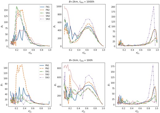
Betti numbers estimated from the δTb field for all our reionization models when observed with SKA-Low. The top and bottom panels represent the Betti number curves extracted from mock observations of tobs = 1000 h (B = 2 km) and tobs = 100 h (B = 1 km), respectively. Different models are marked with different line-styles that are shown in the legend.
We also compare the Betti number curves for all our reionization models in our more pessimistic scenario. The bottom panel of Fig. 10 gives the curves derived from mock observations at tobs = 100 h and B = 1 km. Even though the curves are noisy, we can discern the expected evolution of the Betti numbers for each model. These curves are more reliable at epochs |$x^\mathrm{v}_\mathrm{H\, \rm {ii}}\gtrsim 0.5$|, making it difficult to derive a fit for the evolution of β0. In Table 3 contains the fit parameters for the β1 and β2 curves. As the late neutral islands tend to be large, we find that we can measure the topology of reionization at late times quite well. As noted above, this can even be done using relatively short observations times with SKA-Low.
7 SUMMARY
In this work we explored a new method to study the 3D topology of H ii regions during reionization, namely the three Betti numbers. In the perspective of the distribution of ionized regions the zeroth Betti number (β0) gives the number of isolated H ii regions, the first Betti number (β1) gives the number of neutral tunnels through ionized regions, and the second Betti number (β2) gives the number of neutral islands embedded in ionized regions.
We investigated the evolution of the Betti numbers in a small set of fully numerical and semi-numerical simulations and found a characteristic pattern in which each of the Betti numbers first rises and then falls, each attaining a maximum value at different stages of reionization. When reionization starts, most of the ionized bubbles are isolated and β0 is the largest of the three numbers. It initially rises as the number of ionizing sources, including individual and clustered sources, grows. However, as existing ionized regions grow and new ones continue to form, they will start to overlap, leading eventually to a decrease of β0.
When substantial overlapping of ionized bubbles starts, more and more of these connected regions will be crossed by neutral tunnels and we consequently observe a rise in the values of β1. The time when the decreasing β0 and the increasing β1 cross corresponds to the appearance of the ionized percolation cluster (Furlanetto & Oh 2016). β1 reaches its maximum value at the middle stages of reionization. During this stage, isolated neutral regions, some of them the remnants of broken up tunnels, become more common and therefore the value of the second Betti number (β2) starts to increase. The time when the β1 and β2 curves cross corresponds to the disappearance of the neutral percolation cluster. During the later stages of reionization β2 reaches its peak value after which it drops as the last neutral islands disappear.
We find that the characteristic evolution of the Betti numbers with the volume-averaged ionization fraction (|$x^{\rm v}_{\rm H\, \rm {ii}}$|) of the Universe is quite well fitted by simple functions, a normal or Gaussian function for β1, and lognormal functions for β0 and β2. Each of these is determined by three parameters specifying the peak amplitude (Ai), peak position (μi), and width (σi) of the curves. Using our suite of reionization simulations, we showed that we can distinguish reionization models by their sets of Betti curves.
On the basis of these results we conclude that the Betti numbers provide a better way to describe the topology of reionization than the much better studied genus or Euler characteristic. Not only do the Betti numbers represent a set of intuitively clear morphological concepts in the context of ionized regions, they also display characteristic evolutionary patterns in which they each distinguish different stages of reionization, and which also appear to fit simple functional forms. Furthermore, their evolution shows a connection with the percolation process characteristic of reionization. As the Euler characteristic can easily be calculated from the Betti numbers, there appears to be no advantage to studying the topology of reionization with it.
The redshifted 21-cm signal probes the distribution of neutral hydrogen gas during reionization. Observations with the future SKA-Low will deliver 3D tomographic data sets consisting of sky images of the 21-cm signal at different frequencies. We explored the prospect of deriving the topology of H ii regions from such data sets. To identify ionized regions in the 21-cm data we use the superpixels method introduced in Giri et al. (2018b). We find that we can retrieve the topology of reionization quite well for middle and late stages of reionization (|$x^\mathrm{v}_\mathrm{H\, \rm {ii}} \gtrsim 0.4$|). At early times, most H ii regions are small and difficult to identify in the mock 21-cm data sets due to a combination of low resolution and instrumental noise. We tested our method for two observation times, 1000 and 100 h. For both cases we could retrieve the evolution of β1 and β2 better than the one for β0. We therefore expect that β1 and β2 in practice will be more robust measures of topology than β0.
All Betti numbers curves derived from the mock 21-cm observations are noisy due to the imperfections of the observational data that do not allow a perfect identification of H ii regions. However when we fit β1 and β2 curves with our three parameter models, the intrinsic values of the model parameters are retrieved quite well. Retrieving the model parameters for β0 is more challenging for the reasons explained above.
We have also compared the topologies determined from mock 21-cm observations constructed from our suite of reionization simulations. We can clearly distinguish between these models for a 1000 h observation with SKA-Low. Determining the evolution of the Betti numbers with a 100 h observation is more difficult. However, we can still distinguish between our models using β1 and β2. As isolated neutral regions are relatively large structures (Giri et al. 2019a), the values of β2 estimated from the mock observations are the least affected by limited resolution and noise.
In this paper we have explored a small set of five reionization simulations, produced by two different codes. One might wonder about the validity of some of our conclusions, e.g. regarding the shapes of the Betti curves. If reionization proceeded inside-out we expect the Betti curves to always show the behaviour we have found: each Betti number peaks at a different time, in the order β0, β1, β2. The reason for this is that for inside-out reionization there will be a strong correlation between the local density and the redshift of reionization. The areas of highest density reionize first and the ones of lowest density reionize last. This implies that different stages of reionization can approximately be connected to different threshold values in the density field, where everything above that threshold value is ionized. In this case we expect the evolution of the Betti numbers of ionized regions to approximately follow the Betti curves for different threshold values in a GRF shown in Fig. A1. This means that each Betti number will peak at a different time, in the order β0, β1, β2, just as we have found for all our models. As reionization is a radiative transfer process, the correlation between density and redshift of reionziation will never be perfect, which is why the actual curves are not identical to the more or less Gaussian curves from Fig. A1. Why the evolutionary Betti curves would favour lognormal shapes for β0 and β2 and a Gaussian shape for β1 is harder to explain. We consider our proposed fitting functions to be a useful working hypothesis until cases are found where this approach breaks down.
Our study has used a number of simplifying assumptions which we would like to briefly discuss here. The first is that we have calculated the differential brightness temperature assuming the high-spin temperature limit. If X-ray heating is not as efficient as generally assumed, this assumption may not be globally valid during the earlier stages of reionization. However, as we have seen, the early stages of reionization will anyway be challenging to study topologically as it will be difficult to identify ionized regions in the data.
We have also neglected the various line-of-sight effects when constructing our mock 21-cm observations. These are the LC effect (e.g. Datta et al. 2012) and RSD (e.g. Jensen et al. 2013). The former effect is caused by the evolution of the signal along the frequency direction. If we would analyse 21-cm data sets with a large frequency range (≳ 10 MHz), we would see more overlapping regions at the high frequency end than at the low frequency end. This will affect the topology of H ii regions and therefore the Betti numbers. However, this can be avoided by choosing a narrower frequency range. The RSD effect displaces the signal from its cosmological redshift due to peculiar velocities of gas. This process mostly alters the amplitude of the signal and has a relatively minor impact on the morphology of H ii regions (Giri et al. 2018a) Therefore, we expect only a minor impact on the Betti numbers, specially at the resolution of the telescope. We defer a detailed study of the impact of these line-of-sight effects to the future.
A potentially larger challenge is the impact from bright foreground signals that are many times brighter than the 21-cm signal we want to analyse (Jelic et al. 2008). A good foreground mitigation strategy is crucial to extract the 21-cm signal from radio observation. However, these methods are not perfect and therefore will leave residuals in the 21-cm images. If our structure identification methods struggles to distinguish between these residual foreground and the H ii regions, then studying the topology of reionization would become difficult. In such a case, we have to develop a foreground mitigation method that preserves the topological information. A detailed study of the impact of foreground residual is beyond the scope of this paper.
ACKNOWLEDGEMENTS
We acknowledge Rien van de Weygaert for useful discussion. GM is supported in part by Swedish Research Council grant 2016-03581. The computations were enabled by resources provided by the Swedish National Infrastructure for Computing (SNIC) at PDC partially funded by the Swedish Research Council through grant agreement no. 2018-05973. We also have used results obtained using the Partnership for Advanced Computing in Europe (PRACE) Research Infrastructure resources Curie based at the Très Grand Centre de Calcul (TGCC) operated by CEA near Paris, France, and Marenostrum based in the Barcelona Supercomputing Center, Spain. Time on these resources was awarded by PRACE under PRACE4LOFAR grants 2012061089 and 2014102339 as well as under the Multi-scale Reionization grants 2014102281 and 2015122822.
DATA AVAILABILITY
The data underlying this article will be shared on reasonable request to the corresponding author.
Footnotes
The configuration is described in document SKA-TEL-SKO-0000557 Rev 1 and the positions of the individual stations in document SKA-TEL-SKO-0000422 Rev 2, both retrievable at https://astronomers.skatelescope.org/documents/
This should perhaps be called a depercolation event as the neutral percolation cluster disappears.
REFERENCES
APPENDIX A: TOPOLOGY OF GAUSSIAN RANDOM FIELD
In this section we use a GRF to validate our Betti numbers estimator for digital data. Our GRF is constructed from a (300)3 data cube filled with Gaussian random numbers. Due to discretization, our data cube will not be a perfect GRF. Therefore, following Park et al. (2013) we smooth this data with a Gaussian filter with a FWHM of five cell widths.
We identify structures by putting a threshold on the intensity values. All the pixels below the threshold constitute the structure whose topology we want to study. For any field |$\mathcal {A}$| the thresholds will scan through all the intensity values. Therefore, we will get a set of Betti numbers corresponding to a set of threshold values. The set of thresholds ν is defined such that |$\mathcal {A} = \sqrt{\left\langle \mathcal {A}^2 \right\rangle } \nu + \left\langle \mathcal {A} \right\rangle$|.
The solid curve in Fig. A1 shows the Euler characteristic (χ) curve of the GRF. The χ curve is an even function with two peaks and one trough that follows a fixed analytical form (see Doroshkevich 1970; Tomita 1986). Giri et al. (2019a) already showed that the χ curve derived by our estimator for digital data matches this analytical form.
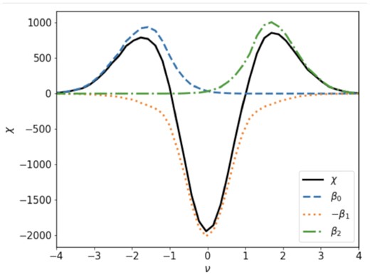
The Euler characteristics χ (solid, black) and Betti numbers β0 (dashed, blue), β1 (dotted, red) and β2 (dash–dotted, green) of a Gaussian random field calculated for various threshold values ν.
Fig. A1 also shows the Betti numbers βκ as a function of threshold ν as determined with our estimator (see Section 2.2). The dashed, dotted, and dash–dotted curve are β0(ν), β1(ν), and β2(ν), respectively. We see that the left peak of the χ(ν) curve is caused by the peak in β0 or a large number of components compared to tunnels and cavities. Similarly, the right peak in χ is associated with a large value of β2 or a large number of cavities compared to components and tunnels. The trough in the χ(ν) curve is due to the value of β1 or a large number of tunnels compared to components and cavities. The Betti curves for a GRF estimated with our method agree with those found in previous works. As far as we know no analytical forms exist for these βκ(ν) curves. See Park et al. (2013) and Pranav et al. (2019) for a more extensive description of the Betti numbers of GRFs.
