Apsidal asymmetric-alignment of Jupiter Trojans

ABSTRACT

1 INTRODUCTION

Presently there are 14 extreme Kuiper belt objects (KBOs) discovered with semimajor axes exceeding 250 au (e.g. Brown, Trujillo & Rabinowitz 2004; Chen et al. 2013; Trujillo & Sheppard 2014; Sheppard & Trujillo 2016). It was noted that all these objects are clustered both in the longitude of perihelion and in the longitude of ascending node, and the confidence level can be as high as |$99.8{{\ \rm per\ cent}}$| (Brown & Batygin 2019). This distinct orbital feature leads to the existence of an additional planet, referred to as Planet 9, which resides on a highly eccentric and inclined orbit (Batygin & Brown 2016; Batygin et al. 2019). The secular perturbation of Planet 9 can be a dynamical mechanism that forces the orbital alignment of the known extreme KBOs, as well as the effect of its mean motion resonances (MMRs; Beust 2016).

We then speculate that the similar orbital alignment could possibly be observed elsewhere much closer to the Sun in the Solar system. For instance, for some known planet moving on the eccentric orbit, it could also confine the apsidal configuration of the objects trapped in its MMRs. The first planet came into our thought is Jupiter, which has the largest mass and a relatively large eccentricity (e_J = 0.05) among the four outer planets. Thus we intend to reinvestigate the orbital structure of objects in the low-order MMRs with Jupiter.

The Jupiter Trojans share the semimajor axis of Jupiter, around the leading (L4) or trailing (L5) triangular Lagrangian point, and they are said to be settled in the 1:1 mean motion resonance (MMR) with Jupiter. This population comprising thousands of observed asteroids is currently the second largest group of minor planets in the Solar system, only fewer than the main belt asteroids. As such a large group of small bodies, they may serve as a good field experiment for the dynamical theories developed for Planet 9. It is also well known that the 2:1 Jovian MMR contains a population of asteroids, i.e. the so-called Hecuba gap centred at ≈3.27 au (Schweizer 1969). Although the number of this resonant population has increased to several hundreds, merely 124 objects (i.e. Zhongguos) were identified on stable orbits by Chrenko et al. (2015). So these stable Zhongguos are too few to be used for the statistical analysis at present, and their orbital distribution would not be discussed in this paper.

Over the past decade, many studies have been done for better understanding of the physical and orbital distributions of the Jupiter Trojans. The Wide-field Infrared Survey Explorer (WISE) project has provided the most complete measures of physical properties for approximately 1900 Jupiter Trojans down to ∼10 km (Grav et al. 2011, 2012). According to the size and colour observations, the Trojans are proposed to originate from the same primordial population as the Kuiper belt objects (Fraser et al. 2014; Wong & Brown 2016). While as for the albedo distribution, this property shows no statistical difference between the L4 and L5 swarms, probably indicating the identical chemical and dynamical evolutions (Emery, Burr & Cruikshank 2011). A more exhaustive review can be found in Emery et al. (2015).

The known Jupiter Trojans have been better characterized in terms of their orbital features, and accordingly they were thought to be captured into the Lagrangian regions from the primordial planetesimal disc during the mass growth of Jupiter, by the dissipative forces such as gas drag or collisions (Shoemaker, Shoemaker & Wolfe 1989; Kary & Lissauer 1995; Marzari & Scholl 1998; Fleming & Hamilton 2000; Kortenkamp & Hamilton 2001). However, this process can not explain the broad inclination distribution of the Jupiter Trojans up to 40^○, which was later reproduced in the framework of the Nice model (Tsiganis et al. 2005). Once Jupiter and Saturn crossed their mutual 1:2 MMR, there was a period of time that the planetesimals can be scattered and trapped around L4 and L5 through chaotic paths, and acquire large inclinations; also, the observed orbital distributions of the eccentricity and libration amplitude can be successfully generated (Morbidelli et al. 2005).

Nevertheless, an outstanding issue remains, i.e. the number difference between the two Trojan swarms. With the samples detected by the WISE, Grav et al. (2011) estimated a number ratio of N(L4)/N(L5) ∼1.4 ± 0.2. As a matter of fact, even the possible selection effects are involved, there are still significantly more Trojans in the L4 swarm (Szabó et al. 2007). Recently, Di Sisto, Ramos & Gallardod (2019) calculated the difference in the escape rate between the L4 and L5 Trojans, which is only as small as |${\sim}2{{\ \rm per\ cent}}$| over the age of the Solar system. In additional, Hellmich et al. (2019) considered the Yarkovsky force on the Jupiter Trojans, since only objects with radii ≤1 km are significantly influenced, the number asymmetry existing at large size can not be explained. Consequently, the source of the asymmetry problem should be due to the initial capture implantation, but not the later long-term dynamical evolution. For instance, the Jumping Jupiter and capture mechanism started at ∼3–10 Myr after the birth of the Sun could potentially create a number ratio of N(L4)/N(L5) = 1.3–1.8 (Nesvorný, Vokrouhlický & Morbidelli 2013).

Since the small Trojans with absolute magnitudes H > 11 are far from observationally complete, their intrinsic distributions need to be further improved by increasing the number of the observed samples. According to our previous work (Li & Sun 2018), the total number of Jupiter Trojans with diameters >1 km (i.e. H ≲ 19) is estimated to be approximately half a million. This suggests that there is a huge Trojan population yet to be discovered in future surveys. Hence, it is of special interest to investigate that whether the orbital orientation of the Jupiter Trojans has some particular characteristic. As we know, in the papers published so far for the various distributions of the Jupiter Trojans, the longitude of perihelion and ascending node have not been explicitly considered. If the clustering of either of these two orbital orientations can be detected, it can directly place constrains on preparing the future observation plans.

The rest of this paper is organized as follows. In Section 2, we reveal the apsidal asymmetric-alignment of the observed Jupiter Trojans. In Section 3, we develop the theoretical approach to understand the dynamical mechanism that accounts for this anomalous orbital structure of the Jupiter Trojans, and correspondingly a detailed explanation is provided. In Section 4, we perform numerical simulations to reproduce the apsidally aligned Trojans, sculpted by the eccentric orbit of Jupiter, from an initially uniform distribution of the longitudes of perihelia. The conclusions and discussion are given in Section 5.

2 ORBITAL ORIENTATIONS OF OBSERVED JUPITER TROJANS

As of 2020 May 27, there are more than 8100 Jupiter Trojans have been registered in the Minor Planet Center¹ (MPC). This population includes many objects that only have short-arc observations that may induce inaccurate orbit determinations for them. Thus we only select the Trojans that have been observed over multiple oppositions, resulting 7354 in total. To represent the true members of the Jupiter Trojans, we then numerically evolve the orbits of these samples under the perturbations of four planets in the outer Solar system. The planets’ masses, initial positions, and velocities are adopted from DE405, in the heliocentric frame referred to the J2000.0 ecliptic plane at epoch 1969 June 28 (Standish 1998). Then the planets are integrated to the specified epoch of the Trojans. Finally, we compute the orbital evolution of the considered Trojans.² At the end of the 1-Myr integration, all of them can survive around the individual Lagrangian points. Then these 7354 multioppositional and stable Jupiter Trojans could be used for our analysis. In this way, we can detect and exclude the possible transient Jupiter Trojans such as P/2019 LD2, which can only stay on Trojan-like orbit for about 10 yr (Hsieh et al. 2021).

Fig. 1 shows the orbital element distributions of the L4 (left-hand column, 4625 in total) and L5 (right-hand column, 2729 in total) populations. It can be seen in the upper two panels that, for either the L4 or L5 swarm of Jupiter Trojans, the clustering in the longitude of perihelion ϖ is readily apparent. A simple way to quantify this apsidal alignment is to compare with the number fraction f_even of an even ϖ distribution. If we have N Trojans in total, since the width of each ϖ bin is adopted to be 30^○, a sample size of N_bin = (30/360)N per bin is expected, i.e. the mean fraction |$f_{\rm even}=N_{\rm bin}/N\approx 0.083{{\ \rm per\ cent}}$|⁠. Considering the random variations about the value of f_even due to counting statistics, the uncertainty from Poisson distribution can be calculated by |$\sigma =\pm f_{\rm even}\times \sqrt{N_{\rm bin}}/N_{\rm bin}$|⁠. Accordingly, in the upper panels of Fig. 1, the horizontal solid and dashed lines are plotted to indicate the mean fraction f_even and its 5σ upper uncertainty, respectively. As the peak of the histograms can achieve the value of ∼0.21 (L5)–0.23 (L4), much higher than the dashed line, the clustering of ϖ shows strong significance over 5σ confidence level. Another key point shown in these two figures is that the number peak corresponds to the bin of ϖ = 30^○–90^○ (300^○–330^○) for the L4 (L5) Trojan swarm, giving a difference of around +60^○ (−60^○) with Jupiter’s longitude of perihelion ϖ_J (indicated by the red line).

Figure 1.

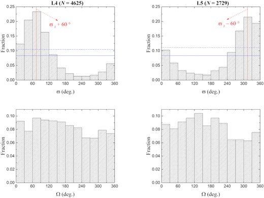
Distribution of the longitudes of perihelia ϖ (upper panels) and the longitudes of ascending nodes Ω (lower panels) of the observed Jupiter Trojans, at the epoch of 2020 May 31. Left-hand column: There are 4625 objects in the L4 region, and the values of their ϖ are clustered around ϖ_J + 60^○ (ϖ_J is the longitude of perihelion of Jupiter). Right-hand column: There are 2729 objects in the L5 region, and the ϖ clustering is around ϖ_J − 60^○. For reference, the horizontal solid lines are plotted in the upper two panels for the uniform distribution in ϖ, and the dashed lines indicate the 5σ upper uncertainty from Poisson statistics.

Open in new tabDownload slide

In order to further confirm the newly found characteristic of apsidal clustering, we need to consider the evolving orbits of Jupiter Trojans at different epoch. Since the periodicity in the variation of Jupiter’s longitude of perihelion ϖ_J is ∼0.17 Myr, we propose that the 1-Myr time-scale is long enough to check the persistence of the apsidal confinement of Jupiter Trojans due to different precession rates of their ϖ. Then the ϖ distribution of the Jupiter Trojans after 1-Myr evolution is shown in Fig. 2, from the integration mentioned at the beginning of this section. One can immediately notice the similar patterns depicted in Fig. 1: (1) the longitudes of perihelia ϖ are clustered around ϖ_J + 60^○ and ϖ_J − 60^○ for the L4 and L5 swarms, respectively; and (2) the number fraction of the clustered samples within a ϖ bin could be over 0.2, which is significantly larger than f_even ∼ 0.083 (>5σ confidence level) in the case of a uniform ϖ distribution. Therefore, the apsidal asymmetric-alignment of Jupiter Trojans should be intrinsic but not due to the observational bias. We suppose that the gravitational perturbation of Jupiter with eccentricity e_J ∼ 0.05 may induce and maintain this intriguing orbital distribution, and an explanation will be offered in the next section.

Figure 2.

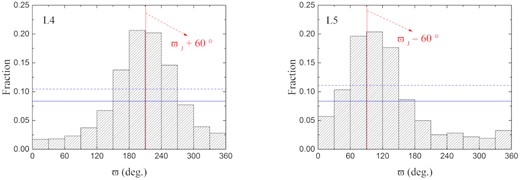
As in the upper two panels of Fig. 1, but for the orbits of the observed Jupiter Trojans after 1-Myr evolution.

Open in new tabDownload slide

However, the longitudes of ascending nodes (Ω) of Jupiter Trojans are not visually clustered in any Ω bin, as shown in the lower panels of Fig. 1. The element Ω measures the azimuthal direction of an object’s orbital plane. Since Jupiter has a very low inclination, which is only about 0|${_{.}^{\circ}}$|3 relative to the invariable plane of the Solar system, this planet could not induce a significant clustering of the orbital planes of its Trojan population. Then it is quite understandable that there appears such a nearly uniform Ω distribution of Jupiter Trojans.

3 APSIDAL CLUSTERING: ANALYSIS

3.1 Theoretical approach

In this subsection, to explore the existence of the apsidally aligned libration islands in the phase space, we consider the spatial elliptical restricted three-body problem (SERTBP) that consists of the Sun, Jupiter and a Jupiter Trojan. Since Jupiter Trojans reside in the 1:1 MMR with Jupiter, for such a co-orbital motion, the classical theoretical approach via the expansion of the disturbing function would fail (see Murray & Dermott 1999, chapter 6). Nevertheless, some new analytical treatments have been developed, such as the secular theories in Morais (1999) and Namouni (1999), the perturbative scheme in Nesvorný et al. (2002), and the symplectic mapping model in Lhotka, Efthymiopoulos & Dvorak (2008). Here we adopt a semi-analytic way to evaluate the resonant disturbing function with no expansion. We refer the reader to Gallardo (2006) for more details on the following calculations.

We assume that the critical argument ψ is fixed at the classical Lagrangian point, i.e. ψ = λ − λ_J = 60^○ for L4 or ψ = λ − λ_J = −60^○ for L5. Under such a typical assumption (Nesvorný & Dones 2002), the dynamical model determined by equation (7) reduces to a system of 2 degrees of freedom, in which Δϖ and Ω are the associated angular coordinates. As a consequence, for a given pair of (i, Ω), the global dynamical behaviors of Jupiter Trojans can be displayed by the level curves of the Hamiltonian in the pseudo phase space (e, Δϖ).

Fig. 3 presents the phase space structure in (e, Δϖ) near Jupiter’s 1:1 MMR, for the Lagrangian point L4. Corresponding to the planar case (i.e. i = 0), Fig. 3(a) shows that there exists a stable equilibrium point at Δϖ ≈ 60^○. The apsidally aligned libration islands found here are consistent with the results from Nesvorný & Dones (2002), and this could validate the Hamiltonian model adopted in this paper. Then we further consider the spatial co-orbital motion, the inclinations are fixed at large values of i = 20^○ and 40^○, given two representative longitudes of ascending nodes (Ω = 0° and 90^○). The resulting portraits (Figs 3b–d) show that, even in the highly inclined cases, the equilibrium point of Δϖ still exists around 60^○, while the shapes of the libration islands may twist. Actually, according to our extra tests, the existence of such an equilibrium point is independent on the orbital elements i ≤ 40^○ and Ω ∈ [0°, 360^○]. Taken in total, the theoretical approach indicates that the L4 Trojans can keep their orbital ellipses oriented with ϖ ≈ ϖ_J + 60^○, leading to the apsidal asymmetric-alignment depicted in Figs 1 and 2.

Figure 3.

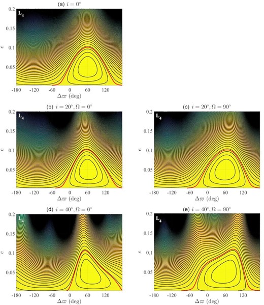
The phase space structure near Jupiter’s 1:1 MMR for the Lagrangian point L4, for the planar case of i = 0, and the inclined cases of i = 20^○, 40^○ and Ω = 0°, 90^○ (see the labels in individual panels). It shows that there is always a stable equilibrium point around Δϖ = ϖ − ϖ_J = 60^○ for the L4 Trojan swarm. The red curve indicates the separatrix dividing the libration and circulation regions. In the calculation of the Hamiltonian by equation (7), the eccentricity e_J of Jupiter is taken to be its real value of 0.05.

Open in new tabDownload slide

We notice that the median eccentricity e_m in the libration island is about 0.05, which likely corresponds to Jupiter’s eccentricity (e_J = 0.05). As a matter of fact, Nesvorný et al. (2002) showed that, in the planar case, e_m is always approximately equal to e_J as the latter artificially increases. This may qualitatively show that Jupiter’s eccentric orbit does control the apsidal configuration of its Trojan population. Then we have to point out that, as long as the real value of e_J = 0.05 is adopted, the libration islands locates below the separatrix going through a critical eccentricity of e_c ≈ 0.1 (see the red curve in Fig. 3a). This suggests that the Jupiter Trojans trapped in the apsidally aligned libration islands should have the maximum e smaller than 0.1, otherwise Δϖ may experience a full circulation between 0° and 360^○. While we find that the condition e < e_c ≈ 0.1 can only be fulfilled for a small fraction (⁠|${\sim}20{{\ \rm per\ cent}}$|⁠) of the observed Jupiter Trojans, and some objects with current osculating e < 0.1 may cross this upper limit during the long-term evolution. Besides, the inclinations of the Trojans are evolving with time but not steady, this could somewhat affect the profiles of the level curves on the phase space (e, Δϖ) as indicated by Figs 1 and 2. Therefore, in order to quantitatively understand the apsidal alignment phenomena, further investigation is clearly warranted.

For the Lagrangian point L5, the corresponding phase space structures at different i values have also been constructed, as shown in Fig. 4. It can been seen that, by comparing with Fig. 3 (for the L4 point), these two sets of portraits show symmetry concerning the libration islands: (1) The stable equilibrium points are around Δϖ ≈ −60^○, where the L5 Trojans are clustered as shown in the right-hand panels of Figs 1 and 2; and(2) the other properties of level curves, either in the libration islands or in the circulation regions, are nearly the same. This is not unexpected since the dynamics around the L5 point is a mirror image of the L4 point in the restricted three-body problem. Furthermore, as noted in Section 1 and some other previous works (Nesvorný & Dones 2002; Di Sisto, Ramos & Beaugé 2014; Holt et al. 2020), under the gravitational effects of the four outer planets, the L4 and L5 Trojan swarms show almost the identical dynamical structure and stability in the long-term evolution. We thereby will only consider the L4 Jupiter Trojans in the following sections.

Figure 4.

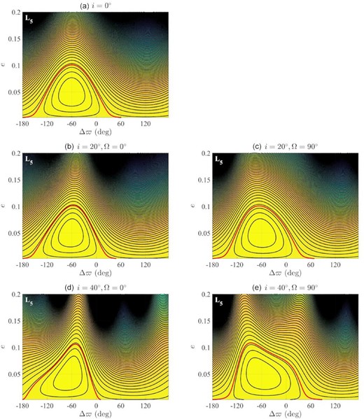
The same as Fig. 3, but for the Lagrangian point L5. It shows that the stable equilibrium point locates around Δϖ = ϖ − ϖ_J = −60^○ for the L5 Trojan swarm.

Open in new tabDownload slide

3.2 Towards the explanation of the observation

From the above semi-analytical results, we deduce that the apsidal alignment should appear for the Jupiter Trojans with e < 0.1. When considering the dynamics of the Jovian Trojans, generally the proper elements are adopted (Milani 1993; Beaugé; & Roig 2001). The proper elements can be understood as the average motion by eliminating the short periodic oscillations from the osculating elements (Morbidelli et al. 2005). Following Morbidelli & Nesvorný (1999) and Lykawka & Mukat (2005), we compute the numerical proper eccentricities e_p by averaging the 2000 yr time-step output from the entire 1 Myr integration³. We then find that, for the observed Trojans having e_p < 0.1, a considerable portion of them actually are not confined by Jupiter's perihelion. We suppose that their osculating eccentricities may not be exclusively small enough (i.e., < 0.1), and the corresponding orbits could temporarily escape the Δ ϖ libration islands as shown in Fig. 3.

In order to characterize the variation of the instantaneous osculating eccentricity, besides the proper value e_p for eccentricity, we additionally introduce the maximum value e_Max. As we mentioned before, hereafter the analysis would be carried out only for the Jupiter Trojans around the L4 point. For the 4625 known L4 Trojans, we split them into three groups according to their eccentricities, and the individual distributions of Δϖ (=ϖ − ϖ_J) at the end of the 1-Myr integration are presented in Fig. 5:

1. Population I. These objects have e_Max < 0.1 during the entire 1-Myr evolution, surely the condition e_p < 0.1 is fulfilled. The total number of this population is N₁ = 1656, i.e. a fraction of |$p_1\sim 36{{\ \rm per\ cent}}$| of the L4 Trojans. Since their eccentricities would never exceed 0.1, theoretically, they are allowed to persistently reside in the islands of Δϖ libration shown in Fig. 3. Consequently, we notice in Fig. 5(a) that almost all of the Population I samples are clustered in the interval Δϖ = 0°–120^○, and the peak matches the theoretical equilibrium point at Δϖ = 60^○.

2. Population II. These objects have e_p < 0.1 but e_Max > 0.1 (N₂ = 2348 and |$p_2\sim 51{{\ \rm per\ cent}}$|⁠). This indicates that they would have their osculating eccentricities occasionally increased to e > 0.1, while for a larger time fraction of the evolution their orbits lie within the e < 0.1 range. Fig. 5(b) shows that the apsidal confinement of Population II is still quite noticeable, as the histogram bins around Δϖ = 60^○ could be higher than the dashed line, which indicates a significant variation from a uniform Δϖ distribution (see the solid line) at the 5σ confidence level.

   Nevertheless, Population II has a much less prominent clustering of ϖ than Population I, because during some time intervals they have osculating eccentricities e > 0.1 and populate outside the apsidal alignment islands in Fig. 3. Through a deeper analysis of the orbital evolution of the Population II samples in our numerical integration, we find that the objects located in the vicinity of Δϖ = 60^○ keep changing. That is to say the objects aligned in ϖ at a certain time t₁ could be much different from those at another time t₂. For instance, we considered a subset of Population II with e_Max = 0.11–0.12, which has a total number of 462. From the beginning of the integration, there are 88 objects trapped in the region of Δϖ = 60^○ ± 20^○ at t = 0.1 Myr, and 105 such apsidally aligned objects are identified at t = 1 Myr, but only 11 are the same ones.

3. Population III. They have larger e_p > 0.1 (N₃ = 612 and |$p_3\sim 13{{\ \rm per\ cent}}$|⁠) and spend a considerable fraction of time outside the theoretical libration islands of Δϖ. Naturally, the distribution of Δϖ shown in Fig. 5(c) becomes rather flat by comparing with Fig. 5(b). Nevertheless, we cannot fail noticing that although the apsidal alignment of Population III is weak, but still visible. We determined a lower significance limit at about 2σ uncertainty, as indicated by the dotted line. So why not their ϖ could disperse well enough to be close to a uniform distribution (represented by the solid line)? The reason should be attributed to the fact that the objects with minimum eccentricities larger than 0.1, i.e. could hardly experience the Δϖ libration phase, are as few as |${\lt}1{{\ \rm per\ cent}}$| among Population III.

Figure 5.

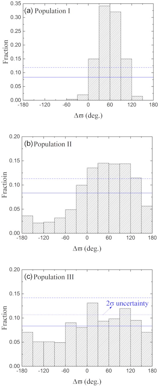
Distribution of the difference of the longitudes of perihelia (Δϖ = ϖ − ϖ_J) between a subset of L4 Trojans and Jupiter: (panel a) Population I with maximum eccentricities e_Max < 0.1 during the 1-Myr evolution; (panel b) Population II with e_Max > 0.1 but proper eccentricities e_p < 0.1; (panel c) Population III with e_p > 0.1. The number fraction of a uniform Δϖ distribution, and its 5σ upper uncertainty are also indicated by the horizontal solid and dashed lines, respectively. In the bottom panel, the 2σ uncertainty is additionally plotted as the apsidal clustering is weaker for Population III.

Open in new tabDownload slide

Figure 6.

For the Jupiter Trojans with proper eccentricities e_p < 0.1 from Population I and Population II, as a function of their maximum eccentricities e_Max, the time fraction T_frac that they spend in the range of |Δϖ − 60^○| < δ = 30^○ (orange), 40^○ (green), 50^○ (blue), and 60^○ (red). The dashed line with the corresponding colour shows that, if the apsidal confinement does not emerge, the Trojans would have a fixed time fraction within the range of |Δϖ − Δϖ₀| < δ for any Δϖ₀ ∈ [0°, 360^○].

Open in new tabDownload slide

The most important result depicted in Fig. 6 is that, for these Trojans, the temporal variation in ϖ is far from uniform. Taking the case of δ = 60^○ for example, the red curve always lies above the red dashed line, meaning that a Trojan with e_p < 0.1 would have its ϖ stuck in a narrow region centred on ϖ_J + 60^○ for a considerable fraction of time. As a result, through a global view of the Trojan population at any specific moment, we would observe the apsidal clustering of their orbits. This phenomenon could be analogous to the spiral arms in galaxies, which is not merely a static accumulation of stars and dust, as explained by the density wave model (Lin, Yuan & Shu 1969). Especially, for the Population I samples with e_Max < 0.1 (i.e. the condition e < e_c ≈ 0.1 is always satisfied), they could be trapped in the range of Δϖ = 60^○ ± 60^○ = 0°–120^○ over a time fraction of |$T_{\rm frac}\gt 80{{\ \rm per\ cent}}$|⁠. Such a large T_frac can nicely explain the prominent components of Population I confined in this very Δϖ range (see Fig. 5a).

Additionally, the profiles of the curves in Fig. 6 show that T_frac decreases as a function of increasing e_Max. Since the osculating eccentricity of a Trojan’s orbit evolves with time, the maximum value e_Max can represent a particular level curve in the phase space (e, Δϖ), as displayed in Fig. 3. When e_Max becomes larger, the libration island centred on the equilibrium point at Δϖ = 60^○ will be increasing in size, leading to fewer part of it located inside a given Δϖ range. Correspondingly, for the orbit in the physical space, it would be confined in the region |Δϖ − 60^○| < δ for a smaller time fraction T_frac. And obviously, the value of T_frac is increasing with the width of the variation in Δϖ, as characterized by the parameter δ.

In summary, the vast majority of the observed L4 Trojans have proper eccentricities e_p smaller than 0.1, and they are evolving on the orbits with osculating eccentricities e < 0.1 for a large period of time in which they could wander inside the libration islands of Δϖ. This scenario could account for the apsidal confinement of the entire Trojan population.

4 APSIDAL CLUSTERING: REPRODUCTION

The planetesimals could have been chaotically captured into Jupiter’s co-orbital regions during the early evolution of the Solar system within the Nice model (Morbidelli et al. 2005; Tsiganis et al. 2005). At the end of this process, their longitudes of perihelia should cover all values of ϖ = 0°–360^○. Therefore, we would like to investigate that whether the apsidal asymmetric-alignment of the currently observed Jupiter Trojans, could be generated from an even ϖ distribution in the later long-term evolution. As the study in the previous sections is indicative of this peculiar orbital structure, the numerical experimentation is to be carried out to evaluate the effect of the secular perturbation of the eccentric Jupiter.

In this section, we still adopt the present outer Solar system model, consisting of the Sun and four giant planets (i.e. Jupiter, Saturn, Uranus and Neptune). As in recent dynamical explorations of the Jupiter Trojans (e.g. Hellmich et al. 2019; Holt et al. 2020), to construct robust simulations, we follow the long-term evolution of 30 000 test Trojans around the L4 point. Initially, all particles have the same semimajor axis (a ≈ 5.2 au) with Jupiter. And similar to the observed Trojan population, they have e ranging from 0–0.3 and a broad inclination distribution of i = 0°–40^○. The initial orbital angles are chosen such that particles start from Ω = 0 and ψ = λ − λ_J = 30^○–90^○, while the values of their ϖ are randomly selected between 0° and 360^○. We then monitor the orbital evolution of these test Trojans in the long-term numerical integration.

Bearing in mind that, for Jupiter, the periodicity in the variation of its longitude of perihelion ϖ_J is about 1.7 × 10⁵ yr. So given a relatively shorter time-scale of 10⁵ yr, in the top panel of Fig. 7, we provide the first glance at the evolving distribution of Δϖ = ϖ − ϖ_J. At this moment, there are a total of 26 117 particles (i.e. |$87.1{{\ \rm per\ cent}}$|⁠) found on Trojan orbits, characterized by the librating critical arguments ψ. We notice that, although the distribution of Δϖ is seemingly accumulated around 60^○, it is, in fact, very close to the uniform distribution indicated by the solid line.

Figure 7.

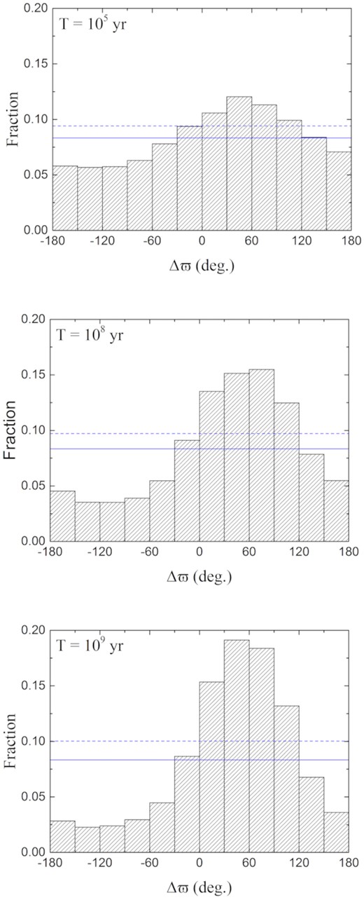
For simulated Jupiter Trojans starting with longitudes of perihelia chosen uniformly in the range of ϖ = 0°–360^○ (equivalent to Δϖ = ϖ − ϖ_J = 0°–360^○), the evolving distribution of Δϖ at t = 10⁵ (top panel), 10⁸ (middle panel), and 10⁹ yr (bottom panel). The solid and dashed lines represent the uniform distribution of Δϖ and the 5σ significance, respectively.

Open in new tabDownload slide

As the time passes, due to the secular perturbation of the eccentric Jupiter, the simulated Trojans can reach the orbits that are more and more apsidally aligned. At the epoch of 10⁸ yr, as shown in the middle panel of Fig. 7, the clustering in Δϖ is quite obvious. And when the integration ends at 10⁹ yr, on the order of the age of the Solar system, there remain 10,417 objects (i.e. |${\sim}34.7{{\ \rm per\ cent}}$| of initial samples) librating around the L4 point. For these simulated Trojans, as shown in the bottom panel of Fig. 7, the largest fraction of objects clustered adjacent to the location of Δϖ = 60^○ is as high as ∼0.2. We recall that the distribution of the longitudes of perihelia of the observed L4 Trojans, as displayed in the left-hand panels of Figs 1 and 2, also has a comparable peak next to the same location.

For each set of 3000 test Trojans, we choose the mean μ to be one of four representative values of 0°, 90^○, −90^○, 180^○, and the associated Δϖ distribution is plotted in the left-hand column in Fig. 8 (from top to down). We can see that the initial number fraction of test Trojans within the bin next to Δϖ = μ could peak over 0.2. Keeping the other initial conditions of the system, we repeat the 10⁹ yr numerical integrations for the simulated Jupiter Trojans, and the final distributions of Δϖ are summarized in the right-hand column in Fig. 8. The main feature is that, starting from any Δϖ distribution, the simulated Trojans would eventually reach the state of apsidal alignment around Δϖ = 60^○. Through a closer look at the cases of μ = −90^○, 180^○, one notices that although the region near Δϖ = 60^○ was nearly empty (two lower left-hand panels), the expected apsidal alignment of the Trojans within this region can still be seen at the end of the 10⁹ yr evolution (two lower right-hand panels). This provides support for the results obtained from our previous run with an initially uniform Δϖ distribution. We end by noting that the previous run using 30 000 test Trojans is quite ‘expensive’, and more than a month of CPU time is needed. As a matter of fact, we found that an order of magnitude fewer objects could be a sufficient sample size to perform the statistical analysis. Therefore, in order to save computational time, we use a set of 3000 test Trojans (for each μ) for the simulations with different set-up of Δϖ distribution, and the results are considered robust.

Figure 8.

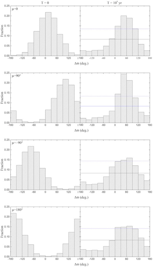
Left-hand column: initial Δϖ of simulated Jupiter Trojans assigning from Gaussian distributions with means of μ = 0°, 90^○, −90^○, 180^○ (from the top to bottom). For the bin next to the location Δϖ = μ, the initial number fraction could peak over 0.2. Right-hand column: the corresponding final distribution of Δϖ after 10⁹ yr evolution. As well, the uniform distribution (solid line) and its 5σ significance (dashed line) are indicated in each panel.

Open in new tabDownload slide

In summary, we conclude that the apsidal asymmetric-alignment of Jupiter Trojans should be a natural consequence of Jupiter’s secular perturbation. The orbital orientations of the Jupiter Trojans at the moment of capture could affect the extent of the clustering in their ϖ, but only slightly and would not alter the overall ϖ distribution. The origin of the Jupiter Trojans still remains uncertain, and a thorough exploration goes beyond the scope of this paper.

5 CONCLUSIONS AND DISCUSSION

This work is inspired by the hypothesis that the eccentric and inclined Planet 9 could cause the orbital clustering of the extreme KBOs beyond 250 au (Batygin & Brown 2016). As Jupiter has a relatively large eccentricity (e_J ∼ 0.05) among the planets in the outer Solar system, for the observed Jupiter Trojans with the number in excess of 7000, we statistically analysed the distribution of their orbital orientations.

It is interesting to find that the L4 and L5 Trojan swarms have longitudes of perihelia ϖ gathered around ϖ_J + 60^○ and ϖ_J − 60^○ (ϖ_J is the longitude of perihelion of Jupiter), respectively. And for the ϖ bins with the width of 30^○, either of these two swarms has a number fraction peaked over 0.2, which is much larger than the fraction of ∼0.083 resulted from the uniform distribution, at the 5σ confidence level from Poisson statistics. This suggests that the apsidal asymmetric-alignment of Jupiter Trojans is noticeable. By integrating the orbits of Jupiter Trojans up to 1 Myr, the clustering in ϖ can persist over time, thus this orbital characteristic should be robust but not due to the observational bias. The apsidal clustering of the Trojans is supposed to be caused by Jupiter that possesses a relatively large eccentricity of e_J ∼ 0.05. However, the distribution of the longitudes of ascending nodes for the observed Trojans is rather uniform, since the inclination of Jupiter is very low.

Next, in the framework of the spatial elliptical restricted three-body problem, we developed a theoretical approach to understand the clustering in ϖ for the Jupiter Trojans. The averaged Hamiltonian with 3 degrees of freedom is derived to describe the dynamics of the 1:1 mean motion resonance. By taking the resonant angle to be ψ = 60^○ (−60^○) for the L4 (L5) Trojan swarm, the Hamiltonian can be reduced to a 2 degrees of freedom system, in which the momenta are in terms of the Trojan’s eccentricity e and inclination i. Then we provide a global view of the dynamical aspects for the co-orbital motion in the phase space (e, Δϖ), where Δϖ = ϖ − ϖ_J. The portraits show that there are equilibrium points at (e ∼ e_J, Δϖ ∼ ±60^○), either for the coplanar or inclined cases with i ≤ 40^○. This can nicely account for the distinctive apsidal asymmetric-alignment of Jupiter Trojans as revealed above. We further note that the apsidally aligned islands of libration exist only for the Trojan-like orbits with e < e_c ∼ 0.1, and this is essentially determined by Jupiter’s eccentricity e_J ∼ 0.05. However, only a small fraction of the known Jupiter Trojans satisfy this eccentricity condition.

For better understanding the influence of the Trojan’s eccentricity, the proper value e_p and the maximum value e_Max are computed in their 1-Myr evolution. Previous studies show that the two Lagrangian points have almost the identical dynamical features concerning the orbits around them, thus we then consider only the L4 Trojans. We introduced a time index T_frac to measure the fraction of time that the L4 swarm has ϖ placed in the range of |Δϖ − 60^○| < δ = 60^○. The results show that, for the population with e_p < 0.1, the derived time fraction T_frac is much larger than the value corresponding to a uniform variation of ϖ in time. It suggests that although some objects evolve to the orbits with osculating eccentricities exceeding 0.1 (i.e. having e_Max > 0.1), and accordingly could temporarily escape the libration islands of Δϖ, they actually spend most of their time in the said Δϖ range. Because the more eccentric Trojans with e_p > 0.1 are very few in number, the entire Trojan population would display the obvious apsidal alignment.

Finally, we proceed to investigate whether Jupiter Trojans could reach this peculiar orbital structure in the long-term evolution. Initially, tens of thousands of test Trojans around the L4 point are uniformly distributed between ϖ = 0° and 360^○, given e = 0–0.3 and i = 0°–40^○. Then by numerical simulations, we compute the evolution of these samples, sculpted by the eccentric Jupiter and the other three planets in the outer Solar system. The orbital distributions obtained at different epochs show that, as time passes, the clustering of the simulated Trojans around Δϖ = 60^○ becomes more and more prominent. And at the end of the 10⁹ yr integration, the number fraction of the apsidally aligned objects is peaked about 0.2, for the Δϖ bins with the width of 30^○, similar to what is observed in the real Trojan population. A series of additional runs, for which the test Trojans have initial ϖ obeying Gaussian distributions with different means, have also been carried out. We find that the similar apsidal alignment around Δϖ = 60^○ can always be reproduced.

In this work, our theoretical approach built on the restricted three-body model suffers from a minor problem: for the 1:1 resonant angle ψ of the co-orbital motion, the libration centre ψ₀ does not fix at the classical Lagrangian point of 60^○ (L4) or −60^○ (L5), but it actually varies with the Trojans’ eccentricities e and inclinations i. By expanding the disturbing function to the fourth order in e and i, Namouni & Murray (2000) studied the orbits librating around L4 or L5 with small amplitudes, and they showed that the displacements of equilibrium points from the equilateral configuration increase as a function of increasing e. The displaced equilibrium points were also calculated for the coplanar configuration of two massive planets in the co-orbital motion (Giuppone et al. 2010). As shown in Fig. 7 of their work, given a ratio m₂/m₁ ≥ 1 of planetary masses, the equilibrium value of ψ (i.e. ψ₀) for the L4 solutions increases with the eccentricity e₁ of the less massive planet. Considering the limit of the mass ratio m₂/m₁ → ∞, i.e. in the restricted three-body problem, this trend is the same as that discovered by Namouni & Murray (2000). By using the semi-analytical method developed in our previous works for the resonant Kuiper belt objects (Li, Zhou & Sun 2014a, b; Li et al. 2020), the libration centre ψ₀ for the L4 co-orbital motion is determined as a function of the massless Trojan’s e for different i. Considering the observed range of e ∼ 0–0.3 and i ∼ 0°–40^○, Fig. 9 shows that ψ₀ could change between 57^○ and 70^○, indicating that the equilibrium point within the apsidal alignment islands (see Fig. 3a) may shift no further than 10^○ from Δϖ = 60^○. Since the L4 Trojans are mainly clustered in a much wider range of Δϖ = 0°–120^○, the ≲ 10^○ displacement of Δϖ would not affect our conclusions. This argument can be supported by the apsidal alignment of Jupiter Trojans from both the observation and numerical reproduction.

Figure 9.

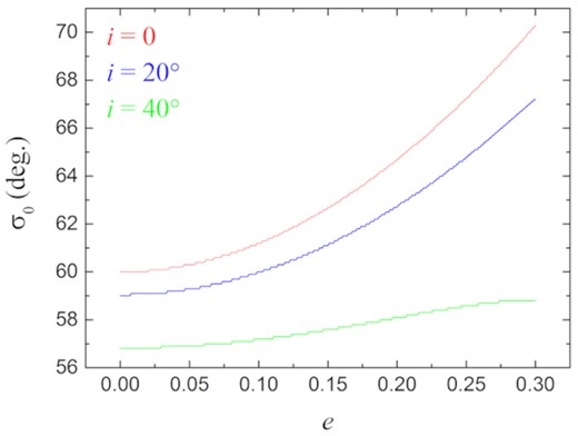
The libration centre ψ₀ of the 1:1 mean motion resonance with respect to the eccentricity e for the inclination i = 0° (red), 20^○ (blue), and 40^○ (green), determined from the circular restricted three-body model.

Open in new tabDownload slide

ACKNOWLEDGEMENTS

This work was supported by the National Natural Science Foundation of China (Nos 11973027, 11933001, 12073011, and 11603011), and National Key R&D Program of China (2019YFA0706601). We would also like to express our sincere thanks to the anonymous referee for the valuable comments.

DATA AVAILABILITY

The data underlying this paper are available in this paper and in its online supplementary material.

Footnotes

REFERENCES