


ABSTRACT
We study the multiple populations of ω Cen by using the abundances of Fe, C, N, O, Mg, Al, Si, K, Ca, and Ce from the high-resolution, high signal-to-noise (S/N > 70) spectra of 982 red giant stars observed by the SDSS-IV/APOGEE-2 survey. We find that the shape of the Al–Mg and N–C anticorrelations changes as a function of metallicity, continuous for the metal-poor groups, but bimodal (or unimodal) at high metallicities. There are four Fe populations, similarly to previous literature findings, but we find seven populations based on Fe, Al, and Mg abundances. The evolution of Al in ω Cen is compared to its evolution in the Milky Way and in five representative globular clusters. We find that the distribution of Al in metal-rich stars of ω Cen closely follows what is observed in the Galaxy. Other α-elements and C, N, O, and Ce are also compared to the Milky Way, and significantly elevated abundances are observed over what is found in the thick disc for almost all elements. However, we also find some stars with high metallicity and low [Al/Fe], suggesting that ω Cen could be the remnant core of a dwarf galaxy, but the existence of these peculiar stars needs an independent confirmation. We also confirm the increase in the sum of CNO as a function of metallicity previously reported in the literature and find that the [C/N] ratio appears to show opposite correlations between Al-poor and Al-rich stars as a function of metallicity.
1 INTRODUCTION
Globular clusters (GCs) are long known to host multiple populations (MPs) of stars that have different chemical compositions. In the last decade, these MPs have been well explored by large spectroscopic surveys (e.g. Carretta et al. 2009a,b,c; Mészáros et al. 2015; Pancino et al. 2017; Masseron et al. 2019; Mészáros et al. 2020; Horta et al. 2020) and photometric (e.g. Piotto et al. 2007; Sarajedini et al. 2007; Piotto et al. 2015; Milone et al. 2017; Soto et al. 2017). Recently, Bastian & Lardo (2018) provided an overview on MPs in GCs.
Even though the MPs in GCs usually have Na, O, Al, Mg, C, and N abundance variations, there are very few GCs known to have a variance in Fe larger than the abundance measurement errors. One such cluster is ω Cen having stars with a wide range in metallicity (−2.2 < [Fe/H] <−0.6), this cluster has been studied in detail by several groups who identified four main populations with different metallicities (Norris & Da Costa 1995; Pancino et al. 2002; Johnson & Pilachowski 2010; Marino et al. 2011). The existence of several populations in ω Cen has led to the conclusion that this cluster was probably massive enough, at some time, to retain the ejecta of supernovae, which would have progressively enriched each new star generation with the Fe produced at the end of each burst of star formation.
The number of populations that exist in ω Cen remains an open question and strongly depends on the selected element or families of elements used to identify these groups. For example, Gratton et al. (2011) identified six populations that belong to three main groups in ω Cen by using the k-means algorithm and the abundances from Johnson & Pilachowski (2010). ω Cen exhibits large star-to-star variations in several light elements, including C, N, O, Na, Mg, Al, and Si and also s-process elements (Norris & Da Costa 1995; Smith et al. 2000; Johnson & Pilachowski 2010; Stanford, Da Costa & Norris 2010; Marino et al. 2012). While this is similar to other regular GCs, ω Cen is unique in the sense that each group in metallicity shows its own Na–O anticorrelation; the more metal-rich populations have a higher percentage of Na-rich and O-poor stars than metal-poor ones, resulting in a slightly more extended Na–O anticorrelation than the one observed in the metal-poor regime (Marino et al. 2011). In addition, a correlation between the sum of CNO and s-process elements with metallicity has also been observed for ω Cen (Johnson & Pilachowski 2010; Marino et al. 2011). The split main sequence in ω Cen is suspected to be accompanied by a large variation in the He content, based on fitting stellar models on Hubble Space Telescope observations (Bellini et al. 2010; King et al. 2012). Helium enrichment also generally correlates with [Na/Fe] and [Al/Fe] (Dupree & Avrett 2013), with classic first population stars having Y < 0.22, in contrast to those stars that are enriched in Na, for which (Dupree & Avrett 2013) found Y = 0.39–0.44.
Considering all the chemical signatures and observational evidences discussed, it is apparent that the formation of ω Cen was probably more complex than any other Galactic GC. It is possible that ω Cen was accreted by the Milky Way but the question remains if ω Cen also interacted with the Milky Way. There are two leading scenarios proposed for the formation of ω Cen; the first is that it is the remnant core of a dwarf galaxy (Bekki & Freeman 2003), and the second a merger of multiple clusters (van den Bergh 1996; Lee et al. 1999). As a combination of the two, modelling of the merging scenario of clusters in a dwarf galaxy has shown great promise lately, as it has been able to reproduce the observed properties of ω Cen (Mastrobuono-Battisti et al. 2019).
The more metal-rich stars in ω Cen are concentrated in the southern part of the cluster. Pancino et al. (2000, 2003) found that the three main stellar sub-populations of ω Cen have different spatial distributions, making it one of the very few clusters currently known in which metal-rich stars have a more extended spatial distribution than metal-poor stars. This spatial coverage was studied in detail by Calamida et al. (2017), who concluded that merging scenario is a viable explanation for the formation of ω Cen. Evidence of interaction with the Milky Way was eventually discovered by Ibata et al. (2019b) who proved with N-body simulations that the ‘Fimbulthul’ structure, a stream of 309 stars that surround the inner Galaxy (Ibata, Malhan & Martin 2019a), is the tidal stream of ω Cen.
In this paper, we will revisit the metallicity distribution of ω Cen in Section 3, examine the shape of the Al–Mg, the N–C anticorrelations, and deep mixing as a function of metallicity in Sections 4 and 7. Our goal is to investigate the formation of ω Cen by deriving abundances of its MPs. We aim to do this by comparing the [Al/Fe] distribution in ω Cen and the Milky Way. These discussions can be found in Sections 5 and 6.
2 THE ω CEN SAMPLE
This study is a continuation of our recent work (Mészáros et al. 2020) analysing APOGEE (Majewski et al. 2017) data in ω Cen. Similarly to our previous studies, we select stars based on their radial velocity and their distance from the cluster centre, but we did not limit the metallicity of the selected stars for ω Cen. In radial velocity, we required stars to be within three times the velocity dispersion of the mean cluster velocity, and in distance we required stars to be within the tidal radius. We also used the average cluster radial velocity and its scatter from Gaia DR2 (Baumgardt & Hilker 2018) rather than from Harris (1996, 2010 edition). In addition, we introduced a fourth step that is based on selecting stars that have proper motion within a 2.0 mas yr−1 range around the cluster average proper motion from the Gaia DR2 catalogue (Gaia Collaboration et al. 2018).
In APOGEE DR16 (Ahumada et al. 2020; Jönsson et al. 2020), there were 243 additional targets belonging to ω Cen that had not been included in Mészáros et al. (2020); these stars are now analysed here. In Mészáros et al. (2020), we only gave a short overview of ω Cen, without separately discussing its populations. The majority of these stars belong to the most metal-poor and most metal-rich populations, making it possible to examine the chemical properties of these populations in more detail than otherwise would have been possible. We derived their atmospheric parameters and used the BACCHUS Masseron et al. (2016) pipeline to obtain their chemical abundances. The exact same set-up from Masseron et al. (2019) and Mészáros et al. (2020) was used, such that the results from these additional targets (207 of them with S/N > 70) are on the same scale and can be merged with the previous results from Mészáros et al. (2020) in order to further examine the statistics of MPs in ω Cen. Similarly to Masseron et al. (2019) and Mészáros et al. (2020), we used Asplund et al. (2009) for our Solar abundance reference table. The complete set of stellar parameters and abundances can be found in Table 1, which includes stars from Mészáros et al. (2020); there are 1141 stars, 982 of them have S/N > 70, compared to 898 stars and 775 with S/N > 70 published in Mészáros et al. (2020). We limit our discussion to stars with S/N > 70, and also apply the same quality assurance cuts in atmospheric parameters as in our previous papers.
Atmospheric parameters and abundances of individual stars.
| 2MASS ID | Cluster | Status | Teff | log g | [Fe/H] | σ[Fe/H] | [C/Fe] | limita | σ[C/Fe] | NC | [N/Fe] | ... |
|---|---|---|---|---|---|---|---|---|---|---|---|---|
| (K) | (cgs) | (dex) | (dex) | (dex) | (dex) | (dex) | (dex) | ... | ||||
| 2M13242154-4738394 | Omegacen | RGB | 4657 | 1.44 | −1.595 | 0.04 | – | 0 | – | 0 | – | |
| 2M13242622-4729383 | Omegacen | RGB | 5594 | 3.51 | −1.214 | 0.12 | – | 0 | – | 0 | – | |
| 2M13243074-4724264 | Omegacen | RGB | 3993 | 0.17 | −1.65 | 0.067 | −0.17 | 1 | 0.046 | 4 | 0.625 | |
| 2M13243844-4736586 | Omegacen | RGB | 4978 | 2.09 | −1.783 | 0.274 | 0.853 | 1 | 0.049 | 1 | – | |
| 2M13244450-4735071 | Omegacen | RGB | 5271 | 2.79 | −1.706 | 0.071 | – | 0 | – | 0 | – |
Notes. This table is available in its entirety in machine-readable form in the online journal. A portion is shown here, with reduced number of columns, for guidance regarding its form and content. Star identification from Carretta et al. (2009b) was added in the last column.
aThe number of lines used in the abundances analysis from BACCHUS (Masseron, Merle & Hawkins 2016).
A comparison of the average Fe, Al, Mg+Al+Si, N, and C+N+O abundances obtained for entire sample of ω Cen stars with the previous results for the smaller sample in Mészáros et al. (2020) is presented in Table 2. Overall, the changes in the abundance averages resulting from the addition of the studied 243 targets to the Mészáros et al. (2020) sample do not change the averages beyond the uncertainties and do not affect the science results of Mészáros et al. (2020). We note, however, that since most of the additional stars belong to the metal-poor or metal-rich population, the scatter of [Fe/H] increased slightly from 0.205 to 0.233 dex; the Al/Fe average abundances decreased by 0.089 dex because the majority of the added stars have low Al abundances, which also leads to a decrease of fenriched (NSG/Ntot) from 0.603 to 0.527. Such changes are expected to appear with more stars added to the sample with new observations, as statistics evolve and become more complete when the sample size increases.
Abundance averages and scatter.
| Parameter | Mészáros et al. (2020) | This paper |
|---|---|---|
| |$N_{\rm 1}\, ^{a}$| | 898 | 1141 |
| |$N_{\rm 2}\, ^{b}$| | 775 | 982 |
| [Fe/H] average | −1.511 | −1.528 |
| [Fe/H] scatter | 0.205 | 0.233 |
| [Fe/H] errorc | 0.077 | 0.079 |
| [Al/Fe] average | 0.586 | 0.497 |
| [Al/Fe] scatter | 0.533 | 0.566 |
| [Al/Fe] average >0.3 dex | 0.935 | 0.927 |
| [Al/Fe] scatter >0.3 dex | 0.389 | 0.442 |
| [Al/Fe] average <0.3 dex | 0.058 | 0.020 |
| |$f_{\rm enriched}\, ^d$| | 0.603 | 0.527 |
| [(Mg + Al + SI)/Fe] average | 0.413 | 0.410 |
| [(Mg + Al + SI)/Fe] scatter | 0.096 | 0.098 |
| [N/Fe] average | 1.273 | 1.334 |
| [N/Fe] scatter | 0.452 | 0.520 |
| [(C + N + O)/Fe] average | 0.642 | 0.699 |
| [(C + N + O)/Fe] scatter | 0.177 | 0.216 |
Note. This table lists statistics for ω Cen from Mészáros et al. (2020) compared to this paper.
The number of all stars in our sample.
The number of stars with S/N > 70.
The average uncertainty of [Fe/H].
fenriched = NSG/Ntot
2.1 The K–Mg anticorrelation
A possible weak anticorrelation between K and Mg in ω Cen was reported in Mészáros et al. (2020). However, this possibility is weakened by the fact that the two K i lines found in the APOGEE region are often blended and also fairly weak at high temperatures and low metallicities. With the addition of a few more stars, the resulting anticorrelation in this study (seen in Fig. 1) is quite similar to what was published in Mészáros et al. (2020); while there are now more stars observed with [Mg/Fe] < 0.1, the anticorrelation signature does not seem to be clearer than in that in Mészáros et al. (2020) as we do not find new stars with high K and low Mg and we still believe that the K enhancement of the Mg-poor stars in ω Cen cannot be convincingly claimed from our measurements.
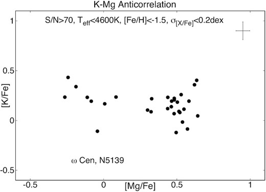
The observed K–Mg anticorrelation in ω Cen.
3 THE METALLICITY DISTRIBUTION
As mentioned in the introduction, many spectroscopic and photometric studies in the literature have demonstrated that ω Cen has a wide spread in metallicity. In particular, the study by Johnson & Pilachowski (2010) presented [Fe/H] measurements for a nearly complete sample of 867 ω Cen giants with V < 13.5, covering the cluster’s full metallicity range. Our sample also covers almost all stars with V < 13.5, but it includes a larger number of stars with V < 16. Their sample consisted of 867 giants, while ours is slightly larger at 982 giants. In Fig. 2, we show the metallicity distribution obtained in this study and as a comparison we also show on the top part of the figure the metallicity distribution from Johnson & Pilachowski (2010). To compare our sample with that of Johnson & Pilachowski (2010), we used the same bin size of 0.05 dex. The general trend in the two metallicity distributions (both obtained from high-resolution spectra) agree quite well: overall the two distributions have a main peak roughly at the same metallicity and a tail that extends to metallicities around −0.5. Johnson & Pilachowski (2010) identified five separate populations based on peaks in their metallicity distribution which are located at: [Fe/H] = −1.75, −1.50, −1.15, −1.05, and −0.75 (the peaks at −1.15 and −1.05 were combined because of the difficulty in de-blending these two populations). Our metallicity distribution is very similar to theirs and four populations can also be identified, which correspond to the following peaks in metallicity: −1.65, −1.35, −1.05, and −0.7 dex. The metallicity peaks in our study are systematically higher by about 0.1 dex than the ones from Johnson & Pilachowski (2010). Such an offset can be considered as quite small, given the very different sets of lines and methodologies used for deriving metallicities from the H band (APOGEE) and the optical spectra (Mészáros et al. 2020). Following Sollima et al. (2005) and accounting for the 0.1 systematic offset in metallicity, these four populations are named: RGB-MP ([Fe/H] < = −1.5), RGB-Int1 (−1.5 <[Fe/H] < = −1.2), RGB-Int2+3 (−1.2 <[Fe/H] < = −0.8), and RGB-a ([Fe/H] > −0.8).

The metallicity distribution of ω Cen. The overall structure can be best fit with four populations with different Fe abundances. Our measurements show a very similar histogram to that of Johnson & Pilachowski (2010) seen in the inset.
4 MPS BASED ON AL AND MG ABUNDANCES
The result of the Mg-Al cycle is observed in almost all GCs that are more metal-poor than [Fe/H] < −1 (Shetrone 1996; Carretta et al. 2009a; Mészáros et al. 2015, 2020).
According to Ventura et al. (2016) an anticorrelation between the abundances of Mg-Al happens because the Mg-Al cycle in high mass AGB stars requires such high temperatures (>70 million Kelvin) to operate that this can only be reached in the core of low metallicity stellar polluters (Ventura et al. 2016). While this AGB scenario explains the shape of the Mg–Al anticorrelation relatively well it does not explain other observed features, for example the Na–O anticorrelation. In fact, none of the currently available models can fully explain all the observed chemical properties of MPs in GCs (Bastian & Lardo 2018). In this paper, we restrict our discussion to the AGB scenario, as most of our discussion lies on the observed properties of Mg and Al abundances of each population. We note, however, that an Al-Mg anticorrelation has been reported for the more metal-rich Bulge GC NGC 6553 (Tang et al. 2017, Schiavon et al. 2017b), and that some atypical Al-rich field stars with [Fe/H] > −1 (although with Mg abundances much lower than GCs of similar metallicity) have been discovered in our Galaxy (Fernández-Trincado et al. 2017; Schiavon et al. 2017a; Horta et al. 2021).
While the shape of the Al–Mg anticorrelation exhibits significant diversity from cluster to cluster (see discussion Mészáros et al. 2020), no GC has an Al-Mg anticorrelation as complex as ω Cen. The Al–Mg abundances for the ω Cen sample are shown in Fig. 3 (left-hand panel), along with the observed Al–Si correlation (middle panel) and the Si–Mg anticorrelation (right-hand panel). The general shape of these trends is very similar to what was presented in our previous study (Mészáros et al. 2020), even though we have roughly 25 per cent more stars than previously. Masseron et al. (2019) discovered that some stars in M15 and M92 show an extreme Mg depletion with some Si enhancement, while at the same time being Al depleted relative to the most Al rich stars in these clusters, displaying a turnover in the Al-Mg diagram. Later, Mészáros et al. (2020) found the same effect for ω Cen, using a smaller sample size than the one used here. We explained the presence of this turnaround as the partial depletion of Al in their progenitors by very hot proton-capture nucleosynthetic processes occurring above 80 MK temperatures.
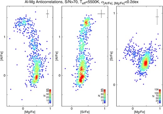
The effect of the Mg–Al cycle in ω Cen colour coded by the number of stars in a ±0.05 dex range around each star. The turnaround of Al abundances at very low Mg abundance values is clearly visible along with density peaks marking various star populations related to star-forming episodes. The average errors are plotted in the top right corner of each panel.
4.1 Metallicity dependence
The complex nature of the Al abundance as a function of metallicity in ω Cen stars has been previously discussed in the literature, for an overview see Johnson & Pilachowski (2010). In this study we derive [Al/Fe] abundances for 873 giant stars (having APOGEE spectra with S/N > 70), allowing us to map the [Al/Fe] abundance distribution in more detail than previous studies (of which, the largest to date is Johnson & Pilachowski (2010), who reported Al abundances for 332 stars in ω Cen).
In Section 3, following the method used by Johnson & Pilachowski (2010), we defined four populations for ω Cen based on the peaks found in the Fe abundance distribution plotted in Fig. 2. In Fig. 4, we now divide the Al–Mg results into these four metallicity groups. Overall, the structure of the Al abundance distribution in this study is very similar to that of Johnson & Pilachowski (2010). The turnover of [Al/Fe] at low values fo [Mg/Fe] is observed only in the most metal-poor group, RGB-MP, below [Fe/H] < −1.5, again confirming that the very hot Mg-Al burning only occurred in metal-poor AGB stars. The extended sample (see Section 2) adds more stars to this most metal-poor population and confirms the existence of the turnaround of Al abundances in ω Cen.
![The Mg-Al anticorrelation for each population defined in the metallicity histogram. The shape of the anticorrelation changes with the metallicity, it is nearly continuous when [Fe/H] < −1.2, then becomes bimodal between −1.2 < [Fe/H] < −0.8 and nearly constant above [Fe/H] > −0.8.](https://oup.silverchair-cdn.com/oup/backfile/Content_public/Journal/mnras/505/2/10.1093_mnras_stab1208/2/m_stab1208fig4.jpeg?Expires=1750097012&Signature=C3sF9~APB5cl~U-N~WMYDDaze-2hfJsrAPedqr6k6hySJUplcy00wq4m~ZZ~slhRbhFHbBNP4arCqg1SLwiYHyAsNsZeFFEXIIR8rPtpwDAyxeBS4VfD2t2TuoRUyGtwlWwKYyfhw2Y34y3jnCkx1NE-ceruzy7hn73Z9RkpRHqgMCaxVn2-fqp042XmPrgOJN16ZcHfdL3KvLtdXAzIeFZIHys2vnZdENpyR79F8HSkHtpUgcnJ3VH-VanHEtT~pU7G8YgyYtaR2~D5E7N6l-0N4UHQSoNZ6pUbvuqonQZWa5yVVsYGgFc56Xik7RdAU8ci~79jCdQGWHF5wZDIuA__&Key-Pair-Id=APKAIE5G5CRDK6RD3PGA)
The Mg-Al anticorrelation for each population defined in the metallicity histogram. The shape of the anticorrelation changes with the metallicity, it is nearly continuous when [Fe/H] < −1.2, then becomes bimodal between −1.2 < [Fe/H] < −0.8 and nearly constant above [Fe/H] > −0.8.
It is apparent that the shape of the Al–Mg anticorrelation changes with metallicity. RGB-MP shows a nearly continuous distribution, while RGB-Int1 becomes more bimodal than continuous and this trend continues to RGB-Int2+3, which is clearly bimodal. The most metal-rich group, RGB-a, shows no significant Al abundance spread. This is similar to what is seen in other metal-rich galactic GCs, with metallicities above [Fe/H] = −0.8, where the Mg-Al burning might not happen, or, its effects may not visible in the logarithmic abundance scale at such high metallicities (Ventura et al. 2016; Mészáros et al. 2020).
To put the ω Cen results discussed above in context we note that bimodal clusters are observed at various metallicities (Carretta et al. 2009a; Mészáros et al. 2015, 2020), but if we consider the 31 clusters in Mészáros et al. (2020), no clear correlation is found between metallicity and the shape of the Al–Mg anticorrelation for clusters with [Fe/H] < −0.9. For example, M53 ([Fe/H] = −1.888) is clearly bimodal, while M5 ([Fe/H] = −1.178) appears continuous. In ω Cen, the Al–Mg anticorrelation apparently becomes more and more bimodal as the metallicity increases. This will be further discussed in Section 5.
4.2 Identifying MPs
While the increased number of analysed stars do not affect the general shape of the Al-Mg anticorrelation, it allows us to analyse the Al histogram in more detail than done by Mészáros et al. (2020). Both the Al–Mg and Al–Si relations have continuous distribution of Al with well-defined density peaks clearly visible in Fig. 3, but the Al histogram by itself is not enough to give a more complete picture of the distribution of Al, as it integrates stars with different [Mg/Fe] and [Fe/H] together. This can be seen in Fig. 5.
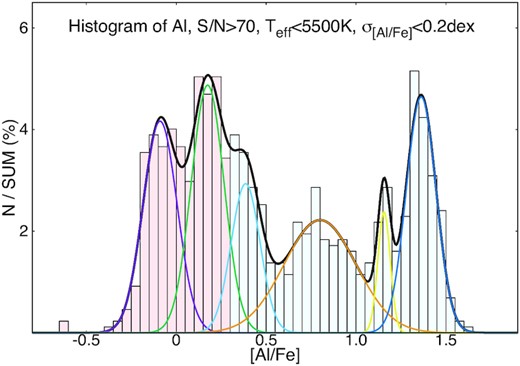
Left-hand panel: The histogram of Al in 0.05 bins in ω Cen. There are six populations identified by fitting Gaussian functions to the Al histogram. These populations are marked on the Al–Si correlation in the right-hand panel, the radius of the circles is equal to the FWHM of the fitted functions.
In Mészáros et al. (2020), three main populations in ω Cen could be distinguished based on their Al abundance distributions, these can now be refined using the extended APOGEE data set. The three populations found previously peaked at around [Al/Fe] = 0.1, 0.75, and 1.4, but now an examination of, for example, the [Al/Fe]–[Si/Fe] correlation (the middle panel of Fig. 3), reveals that the main group centred around [Al/Fe] = 0.1 can be split further into two subgroups. This in contrast with the majority of GCs. In Mészáros et al. (2020), an initial division of FG and SG stars was done with a simple cut at [Al/Fe] = 0.3 dex; such division in [Al/Fe] works well for most GCs in which the effect of Al pollution can be observed. The FG stars with [Al/Fe] < 0.3 could not be divided any further in any of these clusters, within the uncertainties (Mészáros et al. 2020). However, this is not the case for ω Cen.
It is not as straightforward to simply define FG and SG stars in ω Cen as we may be seeing at least six different populations based on the Al histogram. In Fig. 5, six Gaussian functions were fitted to the peaks in [Al/Fe] in the histogram. The first group, originally defined around the peak at [Al/Fe] = 0.1 in Mészáros et al. (2020), is the most numerous and can be divided into three further groups with peaks at [Al/Fe] = −0.09, 0.17, and 0.39. The second group, originally at [Al/Fe] = 0.75, has the widest distribution in Al abundances, but cannot be further split into subgroups using the Al abundances alone; it peaks at [Al/Fe] = 0.8 in Fig. 5. The new APOGEE data more clearly indicate the presence of two peaks in the third group (originally centred around [Al/Fe] = 1.4 Mészáros et al. 2020): one that peaks at [Al/Fe] = 1.16, and another one at [Al/Fe] = 1.36. We note, however, that the latter subgroup is well defined, while the former contains only a few stars.
Similarly to Gratton et al. (2011) we carried out a population analysis using the popular K-means clustering algorithm implemented in R (Steinhaus 1956). We investigated the elements Al, Mg, and Fe, and also tested the addition of Si, which has no effect on the number of populations found. The K-means clustering algorithm revealed the existence of seven populations, or, one more population than found from the analysis of the [Al/Fe] histogram. Fig. 6 shows the distribution of the seven populations in the Fe–Al–Mg space. The difference between the Gaussian peak analysis versus the K-means analysis is limited to the groups with peaks at [Al/Fe] = 0.17, and 0.39 in the [Al/Fe] histogram. These groups split into three sub-groups after the K-means analysis was able to distinguish between groups with different metallicities, resulting in an increase from six to seven populations. The abundance averages and adopted names for the seven populations are found in Table 3.
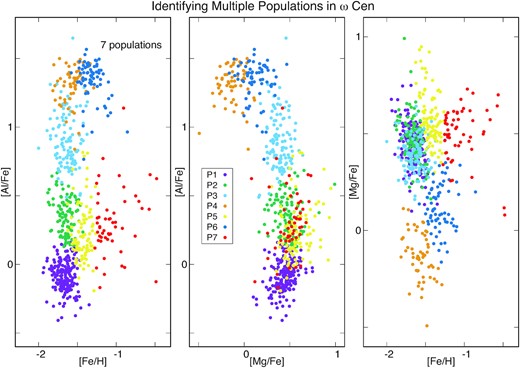
The distribution of stars in ω Cen from seven populations that separates stars in the Fe–Al–Mg abundance space.
Abundance averages of populations.
| Pop. | Na | [Fe/H] | [Mg/Fe] | [Al/Fe] |
|---|---|---|---|---|
| Average | Average | Average | ||
| P1 | 190 | −1.663 | 0.445 | −0.080 |
| P2 | 107 | −1.651 | 0.470 | 0.352 |
| P3 | 107 | −1.634 | 0.388 | 0.898 |
| P4 | 56 | −1.572 | −0.128 | 1.307 |
| P5 | 95 | −1.431 | 0.578 | 0.229 |
| P6 | 68 | −1.312 | 0.124 | 1.334 |
| P7 | 52 | −1.040 | 0.500 | 0.307 |
Notes. This table lists the average [Fe/H], [Mg/Fe], and [Al/Fe] of the MPs in ω Cen.
The number of stars in each population.
By comparing results in this study with those from Gratton et al. (2011) we conclude that the same seven populations found here can be divided into three groups based on their metallicities. This reinforces the findings of the two independent studies, which are based on different sets of elements, Gratton et al. (2011) used [Na/O] and [La/H], while this study [Fe/H], [Mg/Fe], and [Al/Fe]. Populations P1, P2, P3 and P4 belong to the most metal-poor group of stars (Table 3), RGB-MP from Sollima et al. (2005), P5 and P6 have intermediate metallicities, these belong to the RGB-Int1 and RGB-Int2+3 groups, and P7 is the most metal-rich (RGB-a) that is not found to further divided into sub-populations based on our data.
From Fig. 6 we can identify which population is responsible for the turnaround in the Al-Mg anti-correlation discussed in Section 4: the group of stars belonging to the 4th population in our sample, P4, which is shown as orange dots in Fig. 6. Most of stars in P4 belong to the metal-poor population RGB-MP, with some stars from RGB-Int1.
5 MPS BASED ON N AND C
In addition to the Al-Mg anti-correlation, C-N-O-Al abundance relations can also be studied using APOGEE spectra. The N-C and Al-O anti-correlations and the Al-N correlation obtained for ω Cen are shown in Fig. 7 and Fig. 8. These are quite similar to those in Mészáros et al. (2020) despite the increased star count. The N-C anti-correlation, however, is much clearer in our APOGEE data set than previously observed by Marino et al. (2012).
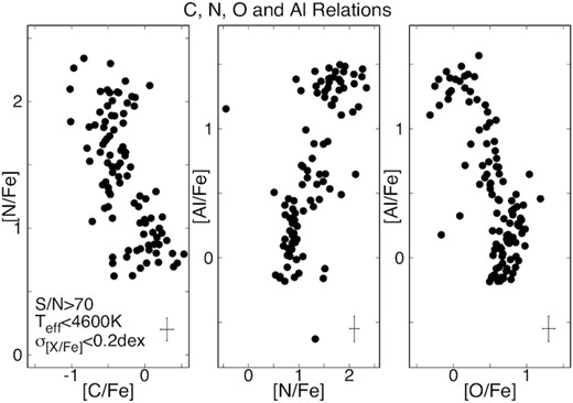
The relationship between C, N, O, and Al in ω Cen. As expected N is anti-correlated with C, while Al is correlated with N, but anti-correlated with O.
![The N-C anti-correlation in the four populations defined from the Fe histogram. The anticorrelation is nearly continuous when [Fe/H] < −0.8, then becomes bimodal above [Fe/H] > −0.8.](https://oup.silverchair-cdn.com/oup/backfile/Content_public/Journal/mnras/505/2/10.1093_mnras_stab1208/2/m_stab1208fig8.jpeg?Expires=1750097012&Signature=G6F8Uh5zdqPtxSaxOL4xsRTsXO27FpowDma3qOsdIAVdwCxc6pp1O1lWtIKPl5UTGgeJzn4g9mosV405Du1XdJ17mD9ZLHbQVrCWJQQpo0JTv9qKSoE3y2OP1ldLg~EJOmSeAQM88NnqnT7qAst92ArM4jaKsXRVPBsEZj6dAqK5Ez2raj7cmRU93LpFn8q922YfDK24heHvIusjzSZA41-koRP5OZpuxRrJ3dZ1RmWFYJHN0tUFYv6GsaKUaMnw-TO2WKHZRHVn6Oaae6aDlnPwNb8wqMCSuygAeVeijXEdfyLugmoIA1qvNiRZVOs9BKP8Q1s1bwdqB1tkYXRBMg__&Key-Pair-Id=APKAIE5G5CRDK6RD3PGA)
The N-C anti-correlation in the four populations defined from the Fe histogram. The anticorrelation is nearly continuous when [Fe/H] < −0.8, then becomes bimodal above [Fe/H] > −0.8.
Similarly to the Al-Mg anti-correlation, the N-C anti-correlation also depends on the metallicity. However, in this study it is not possible to probe the N-C anti-correlation in the most metal-poor groups because the molecular lines of CN, OH and CO disappear in the APOGEE spectra of those stars having metallicities below approximately [Fe/H] < −1.8. The distribution of N abundances are quite continuous for [Fe/H] < −1.2, but becomes bimodal for the most metal-rich stars with [Fe/H] > −1.2. This bimodality occurs in both the N-C and Al-Mg planes and, in both, not at a significantly different metallicity value. There is a difference in the most metal-rich group, RGB-a, which has no significant Al spread beyond our uncertainties, but stars with high N are clearly observed. It is worth noting that some of the stars with high N in the RGB-a population have |$\sigma _[Fe/H]\gt $| 0.2 dex, due to difficulties in fitting molecular lines below Teff < 4200 K.
5.1 Deep mixing
The slope of the N-C anticorrelation is not only affected by the pollution scenario, but also by the deep mixing that occurs on the RGB. The observed slopes discussed above have not been corrected for deep mixing, but ω Cen also shows evidence of mixing as [C/Fe] is strongly correlated with temperature.
Deep mixing can be investigated by probing the variation of [C/N] abundance ratios as functions of metallicity and effective temperature; this is shown in Fig. 9. At first glance the overall value of [C/N] in the studied ω Cen targets appears to be roughly constant with the surface gravity (and also effective temperature) and to a certain degree with metallicity. However, a more complete picture of the behaviour of [C/N] emerges when stars are divided into the FG and SG stars and also considering the [Al/Fe] values (the colour bar in Fig. 9). Stars with low [Al/Fe] generally have high [C/N] ratios, while SG stars with high [Al/Fe] have low [C/N]. This can be understood as the SG stars are formed from gas cloud whose composition has been altered by FG stars, increasing the amount of N and resulting in lower values of [C/N]. The effects of deep mixing does not appear to be visible as a function of surface gravity as [C/N] does not correlate with it, but a slight correlation may exist with metallicity when looking at the FG and SG stars separately. The [C/N] ratios of FG stars increase slightly with increasing metallicity, while the [C/N] of SG stars show the opposite trend, decreasing with increasing metallicity. While the [C/Fe] ratio of SG stars is constant with [Fe/H], the decreasing trend of [C/N] in SG stars comes from the increased [N/Fe] measured for stars with metallicities between [Fe/H] = −1.4 and −1.2. Thus, the correlation seen when looking at only the SG is not the result of deep mixing, but most likely the result of the increased pollution observed at −1.4 < [Fe/H] < −1.2.
![[C/N] as a function of metallicity and surface gravity colour coded by [Al/Fe] to distinguish between FG and SG stars. Correlations in the opposite direction are observed between FG and SG stars as a function of metallicity.](https://oup.silverchair-cdn.com/oup/backfile/Content_public/Journal/mnras/505/2/10.1093_mnras_stab1208/2/m_stab1208fig9.jpeg?Expires=1750097012&Signature=jQ~AgGJknLrdg5GOYaubjdsHb8OLNfQuN7xlOxvgzk-jMLDDneIPsgnTna5BubUvqlnErDafq-yi2tzSt7zxgf~-RoO7ZLoLdUk4Z6rGYNDIt2-0ctzLdsuY7Ftf-sxU4mGu-RmW47R3jy0ouEYxds0jkKhXUJ2K7-YB527dNJe-7Yt7CCbdEcDbAysFVdgWKzMMYCaRY3QLCLSAfQED8cRVVWVSsk6nR5SIbjN04LTtJLtNBsMhSWmVH~ytHaZ~UeYPIh0SvrEK01yUvD74I~UDpG8Ysjqn1WhKWjamx7j7TsRrl35-~8m~JtIEiJIzn6ceRGV05P3OjhOYcDwaog__&Key-Pair-Id=APKAIE5G5CRDK6RD3PGA)
[C/N] as a function of metallicity and surface gravity colour coded by [Al/Fe] to distinguish between FG and SG stars. Correlations in the opposite direction are observed between FG and SG stars as a function of metallicity.
Model calculations by Lagarde et al. (2012) suggest that a drop [C/N] should occur after the luminosity bump at Teff ∼ 4700 K, but this prediction cannot be probed from APOGEE spectra as [C/N] is not measurable at such high effective temperatures. However, ω Cen provides an opportunity to investigate the dependence of deep mixing on metallicity independently of mass, since all stars in ω Cen can be considered to have a very similar mass. Lagarde et al. (2012) also suggested that slightly stronger mixing occurs in more metal-rich stars based on theoretical calculations. This would correspond to the FG stars that exhibit no extra N from pollution from previous populations. Looking at Fig. 9, the [C/N] of FG stars indeed increases slightly with increasing metallicity. While [N/Fe] is constant as a function of metallicity, [C/Fe] is not, so this correlation is the result of increased [C/Fe] at high metallicities seen in Fig. 10. Overall, we conclude that the study of deep mixing is difficult in ω Cen, or in GCs in general, as one has to effectively separate MPs from the deep mixing.
![[C/Fe] as a function of metallicity and effective temperature colour coded by [Al/Fe] to distinguish between FG and SG stars. [C/Fe] of FG stars slightly increases with metallicity.](https://oup.silverchair-cdn.com/oup/backfile/Content_public/Journal/mnras/505/2/10.1093_mnras_stab1208/2/m_stab1208fig10.jpeg?Expires=1750097012&Signature=M3IBhsKavbqJ0NquCoktZDys0jrdH4CQbVAhE0ecfwo~6~eDCaUWMI114TKGchhYbzGtCjLkushQrWqX3kMb5dXmKHH-Dlvbo0EzB1IPHwZuf1tnKhs~qreWVUQPDF7FQEwo7HECEOaQnmHMGXhsxKVKaObgP89K3aZRTxa3cEwG46eqhc5RYt2xkgbnHIl3cN7ra0BnTZy-FRcGlgrJ49DtkELXXkE17nHl0LevBXjRx~YpB7a2ln2oIyuN4Z~p2mDJqe-HTR-1zfHHmYtD9Y85P54VQn~Ciwamtx~n9OxvsmcM3r72sVFm85XllxycbesMlY2fkwU7ujcK88r-0g__&Key-Pair-Id=APKAIE5G5CRDK6RD3PGA)
[C/Fe] as a function of metallicity and effective temperature colour coded by [Al/Fe] to distinguish between FG and SG stars. [C/Fe] of FG stars slightly increases with metallicity.
5.2 C+N+O
The C+N+O in ω Cen has been studied in detail by Marino et al. (2012). They found that [(C+N+O)/Fe] correlates with metallicity and it increases by nearly 0.5 dex from [Fe/H] = −2.0 to −0.9. The sum of C+N+O in this study is shown in Fig. 11 as a function of metallicity and also compared to the Milky Way. Keeping in mind that the metallicity range in which we can analyse the molecular lines in the APOGEE region is more metal-rich than Marino et al. (2012), from [Fe/H] = −1.7 to −0.6, we are able to confirm the their findings that the C+N+O correlates with metallicity. This is driven mostly by the increased amount of O plotted in Fig. 12 (and to a lesser extent, C) at higher metallicities. As there is more C and O in the FG stars, they produce more N explaining the increased N abundances at higher metallicities seen in Fig. 8.
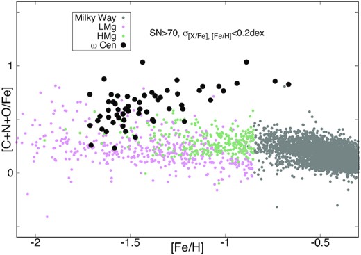
The sum of C+N+O in ω Cen (black dots) and the Milky Way.
![[O/Fe] as a function of metallicity and effective temperature colour coded by [Al/Fe] to distinguish between FG and SG stars. [O/Fe] of FG stars slightly increases with metallicity.](https://oup.silverchair-cdn.com/oup/backfile/Content_public/Journal/mnras/505/2/10.1093_mnras_stab1208/2/m_stab1208fig12.jpeg?Expires=1750097012&Signature=hcwQCFEZ00N8evLp7luS3u4RJpwwd0t8HlYZRGQsKe5aWY15DKK9ymwuRo6dKz~o9BQskiEMXLu4eJdb2pcL~1qjC99LgDMSZP7MbQrw5aiBPGe7xdOVZJnW6vl0X~OK2UohfvGuy-Opz1l8qBYrXbmWqX2G4Hn09u-DoQmULfHuxaO91S6K87mR8hIdzUDuQSd2VBElKDVWAffm6U07HUOybirOMHkl2~jgccDZ~38xkrC26vvp1cwUp2-gVzMq5HWuF8A8zulZtIZ22tXqTtz8xstT79vWQ4DcHlIDBEn2DYB2~cUgSmzHjM1c2v7ZfnQ0cKf9otU-gKFKWxqGOg__&Key-Pair-Id=APKAIE5G5CRDK6RD3PGA)
[O/Fe] as a function of metallicity and effective temperature colour coded by [Al/Fe] to distinguish between FG and SG stars. [O/Fe] of FG stars slightly increases with metallicity.
The existence of the enhanced C+N+O is not currently explained, Marino et al. (2012) could only explain it by SNe coming from an arbitrary initial mass function. Most of the stars with very large C+N+O belong to P7, the most metal-rich population in ω Cen.
6 THE STELLAR POPULATIONS OF ω CEN
6.1 An overview of the seven populations
A comparison of the chemical abundances in Milky Way populations can now be made with the seven populations defined here on the basis of their Al–Fe patterns. The seven populations (P1 through P7) are shown in Figs 13 and 14, where values of [X/Fe] are plotted versus [Fe/H] for nine elements (Al, Mg, Si, Ca, O, C, N, C+N+O, Ce) whose abundances are derived either here or from Mészáros et al. (2020). The small points in these figures represent the Milky Way populations of thin and thick discs (grey), the metal-poor thick disc (green), and halo (pink); the metal-poor thick disc and halo stars are delineated according to the criteria from Hayes et al. (2018) of low-Mg (LMg) and high-Mg (HMg) sequences defining the halo and metal-poor thick disc populations, respectively. In the top left-hand panel of both figures are the values of [Al/Fe] versus [Fe/H], with the seven ω Cen populations identified by colour. Closer examination of the populations confirms the visual impression that P1, P2, P3, and P4 are characterized by a nearly uniform iron abundance; average values confirm this, with 〈[Fe/H]〉P1 = −1.64 ± 0.12, 〈[Fe/H]〉P2 = −1.60 ± 0.11, 〈[Fe/H]〉P3 = −1.64 ± 0.14, 〈[Fe/H]〉P4 = −1.64 ± 0.11. The standard deviations of these values of [Fe/H] are not much larger than the uncertainties in the iron abundances themselves. In this sense, P1, P2, P3, and P4 resemble closely many typical GC populations, which exhibit a large spread in [Al/Fe] abundances, while having only small (if any) [Fe/H] variations. Referring back to Fig. 2, we note that these populations account for ∼2/3 of the ω Cen stars.
![The distribution of [Al/Fe], [Mg/Fe], [Si/Fe], [Ca/Fe], and [O/Fe] as a function of [Fe/H] in ω Cen and the Milky Way. Light green and purple dots represent the HMg (metal-poor thick disc) and LMg groups (halo) in our Galaxy as defined by Hayes et al. (2018). The colouring of the populations in ω Cen is identical to that of the bottom panel of Fig. 6. Unclassified stars are not shown.](https://oup.silverchair-cdn.com/oup/backfile/Content_public/Journal/mnras/505/2/10.1093_mnras_stab1208/2/m_stab1208fig13.jpeg?Expires=1750097012&Signature=nIi25Uw7ypFkSmeapvm6nccG3n1vERIoraLRsCMds3GPQUqVmT2O-NW-lK7IK4VzMgU~FD1vQNQDUWj4BNwVIDKI5WS2ECwJYmMBiJlnBJjbYAYuIYG7veovqiw4dAh3NmyaEzQrz7pVTdQIUxGbOoMd19ChDln7hFrokQhVmpsnj5DMgD-M0k~8jT7GKHSF17RMGF4Qfn4nMYVkbqHbMuEON4ltcKaCkg-WnAYWw8acMs3HmtIlcT-OKs-dQGk0mBeFBPdZYzXKuOpiNlUq3T8iB4WM7Wv1d~eFfX7R~lg~oJhvJDfLs6MS1zD6n12MCA1v9y0OuznhAO7KPyQtYQ__&Key-Pair-Id=APKAIE5G5CRDK6RD3PGA)
The distribution of [Al/Fe], [Mg/Fe], [Si/Fe], [Ca/Fe], and [O/Fe] as a function of [Fe/H] in ω Cen and the Milky Way. Light green and purple dots represent the HMg (metal-poor thick disc) and LMg groups (halo) in our Galaxy as defined by Hayes et al. (2018). The colouring of the populations in ω Cen is identical to that of the bottom panel of Fig. 6. Unclassified stars are not shown.
![The distribution of [Al/Fe], [C/Fe], [N/Fe], [(C+N+O)/Fe], and [Ce/Fe] as a function of [Fe/H] in ω Cen and the Milky Way. Light green and purple dots represent the HMg (metal-poor thick disc) and LMg groups (halo) in our Galaxy as defined by Hayes et al. (2018). The colouring of the populations in ω Cen is identical to that of the bottom panel of Fig. 6. Unclassified stars are not shown.](https://oup.silverchair-cdn.com/oup/backfile/Content_public/Journal/mnras/505/2/10.1093_mnras_stab1208/2/m_stab1208fig14.jpeg?Expires=1750097012&Signature=0tWomnCvz7eOeONdA7AH63rKneNQiXOE9YDALyXNcq~stImGnKH0O0-GG3L8L663S54Sk-qDFIBspqBLpLzU61uqtuvJdiSVm7LrXHFUGnFhGigxBUNvDqYivmQOmoao7dpoaIfjunV~PnBzkGtsxW3Vs3-r2sYQJIWF7t8WvXRPubSl--MRIMIOQHrxNrKcIU3dscWRLiyIdcAgP8qDk3CBsPYntztbo8sqoYRX5f8AmkcFlWTA4I9Mz6BzAsddQhLJ8ra3qksRnozJtEPqDdmPwm~PBjML0dyBhwhFTCvgnKDL~5sfPmZEFkjn~wbsiS753N8sZgWGnIT66ZSUzA__&Key-Pair-Id=APKAIE5G5CRDK6RD3PGA)
The distribution of [Al/Fe], [C/Fe], [N/Fe], [(C+N+O)/Fe], and [Ce/Fe] as a function of [Fe/H] in ω Cen and the Milky Way. Light green and purple dots represent the HMg (metal-poor thick disc) and LMg groups (halo) in our Galaxy as defined by Hayes et al. (2018). The colouring of the populations in ω Cen is identical to that of the bottom panel of Fig. 6. Unclassified stars are not shown.
The remaining three populations identified here (P5, P6, and P7) are more enigmatic in terms of their possible relationship, if any, to the main ω Cen population (P1 through P4). Looking first at their respective Fe abundances reveals that P5 is, within the APOGEE uncertainties, single-valued in iron, with 〈[Fe/H]〉P5 = −1.38 ± 0.04, while P6 and P7 display large ranges in their Fe abundances: 〈[Fe/H]〉P6 = −1.17 ± 0.29 and 〈[Fe/H]〉P7 = −1.05 ± 0.27. Based on the [Al/Fe] and [Fe/H] abundance ratios, P5 and P7 tend to follow the Milky Way halo and thick disc trends, as shown in Fig. 13; however, their [Mg/Fe] values find them falling well above the Milky Way halo and thick disc trends, strengthening the case for ω Cen being a captured system. This trend is born out by the lower panel of Fig. 13, showing that both P5 and P7 also fall well above the Milky Way trends for [O/Fe] versus [Fe/H]. Magnesium and oxygen are produced by, primarily, hydrostatic helium (16O) and carbon (24Mg) burning in massive stars and these overabundances, relative to Fe, in P5 and P7 may indicate significant enrichment from very massive stars, perhaps as a result of a starburst. Unlike P1, P2, P3, and P4, the majority of stars in P5 and P7 do not show evidence of having been formed from material exposed to H-burning via the Mg-Al cycle, although both populations seem to contain a small fraction of Al-rich stars.
Compared to the other populations, P6 is unique in being offset to a higher Fe abundance, when compared to populations P1 through P4, yet composed of stars that were all formed from material that is Al-rich and Mg-poor. It may be that P6 is linked to P1, P2, P3, and P4 by the simple addition of Fe from SN (perhaps SN Ia) increasing [Fe/H] in P6.
Other elements can be used to further illuminate and constrain a picture of chemical evolution within ω Cen. The middle left panel in Fig. 13 shows the behaviour of [Si/Fe], with all populations in ω Cen generally following the Milky Way halo and thick disc evolution. Close inspection does reveal the signature of Si production in P4 and P6, where these populations fall above the trend of [Si/Fe] with [Fe/H] by ∼+0.1 dex. Ventura et al. (2016) find that Si production resulting from H-burning in IMS occurs only in metal-poor ([M/H] ∼ −3.5) massive AGB stars (M ∼ 5 M⊙). The ω Cen results for [Ca/Fe] are quite scattered, likely due to the weakness of the Ca i lines in the APOGEE wavelength window, but follow the Milky Way trends.
Abundances from the heavy s-process element cerium are shown in the bottom panel of Fig. 14 and provide further information on chemical evolution within the ω Cen populations. The populations P1 and P2 have [Ce/Fe] abundances that scatter around values of ∼0.0, while all of the other populations show generally enhanced Ce abundances. Thermally pulsing AGB (TP-AGB) stars are the main producers of the s-process elements, including Ce, pointing to significant contributions from AGB stars to the chemical evolution within ω Cen. Our observation reinforces the findings of Norris & Da Costa (1995), Smith, Terndrup & Suntzeff (2002) who suggested that the pollution from low-mass AGB stars played a crucial part in the evolution of this cluster.
Taken together, the summary abundance results displayed in Figs 13 and 14 provide insights into understanding the stellar populations that constitute the ω Cen system. The pronounced narrow peak in the [Fe/H] distribution (near [Fe/H] ∼ −1.6) in Fig. 2 is composed of stars that display a strong Al–Mg anticorrelation occurring over a very narrow range in Fe abundance (as well as a N–O anticorrelation and an Al–Si correlation), which are signatures that typify many GCs. These stars form the population sequence of P1, P2, P3, and P4, as well as P6 (whose stars have significantly larger Fe abundances and a significant abundance spread): these populations contain over two-thirds of the stars within ω Cen. The populations P5 and P7 have different chemical signatures and do not contain the strong GC Al–Mg anticorrelation. P5 and P7 both exhibit large Fe abundance spreads, as well as [Mg/Fe] and [O/Fe] abundances that fall well above those of the Milky Way halo and thick disk. Both of these populations also exhibit large [Ce/Fe] abundance ratios, with the possibility that P5 and P7 are related stellar systems.
Distilling the abundance patterns in Figs 13 and 14, into, perhaps, the simplest scenario to explain the seven populations defined by the [Al/Fe] abundance ratios would be that ω Cen consists of two general populations. The first population (consisting of P1, P2, P3, P4, and P6) is the underlying GC system that defines the classification of ω Cen as a GC, but one that is very massive and contains a significant spread of Fe abundances (driven by P6). In addition, there is a second distinct population (P5 and P7) characterized by large [hydrostatic-α/Fe] abundances, as well as large s-process abundances. Chemical evolution models would require that P5 and P7 contain material that has been cycled through very massive stars (perhaps a starburst) mixed with ejecta from low-mass TP-AGB stars, which evolve over at least a few Gyr. These two intermingled populations, P5 and P7, within ω Cen presumably represent the central nuclear remnants of a disrupted and captured dwarf galaxy. Such a comparison cannot be made explicitly for ω Cen, as we do not observe the parent dwarf galaxy, but a clear connection between the chemical properties of M54 and the Sagittarius dwarf spheroidal galaxy was explored before showing that interaction between GCs and dwarf galaxies happened in the past (Mucciarelli et al. 2017).
6.2 Comparing with the Milky Way
The discussion in the previous section sketched out possible relationships between the seven ω Cen populations identified here based on their various elemental abundance patterns, a process known as chemical tagging. A comparison of chemical abundances in the ω Cen populations with those of the Milky Way, via chemical tagging, is a useful exercise to illuminate both similarities, as well as differences, in chemical evolution within the two stellar systems. Chemical tagging uses the idea that detailed abundance measurements can be used to identify spatially separated stars that were born in the same molecular cloud, as first presented by Hogg et al. (2016) using APOGEE data. For our chemical tagging, stars from the Milky Way were selected by applying the criteria defined by Hayes et al. (2018) to the DR16 data (Ahumada et al. 2020). Hayes et al. (2018) has divided the metal-poor stars into two groups based on the Mg abundances that are separated from each other by a low density gap. At low metallicities, [Fe/H] < −0.9, the [Mg/Fe] = −0.2 ·[Fe/H] was used by Hayes et al. (2018) to separate the low-[Mg/Fe] population from the high-[Mg/Fe] one. Since we have updated the data to DR16, which has a slightly different abundance scale, this selection function was also updated to [Fe/H] < −0.85 to still avoid most of the thick disk stars, and [Mg/Fe] = −0.29 ·[Fe/H]−0.07 to account for the new position of the gap, which starts to open up in the [Fe/H] = −1.4 to −1.3 range.
It is important to note that while both our analysis and DR16 uses APOGEE data, the abundances were derived independently from each other. Our analysis method is described in detail by Masseron et al. (2019), and the differences amount to about an average 0.1 dex shift in metallicity and 0.2 dex shift in [Al/Fe] between BACCHUS and ASPCAP DR16. These discrepancies also depend on effective temperature, because of differences between photometric and ASPCAP temperatures. We do not calibrate our results to those of ASPCAP, but when doing comparisons between ω Cen and the Milky Way one must keep in mind that such small discrepancies in abundances exist.
Inspection of the various elemental abundances in Figs 13 and 14 reveals that ω Cen is quite different in the behaviour of most elements as a function of Fe abundance. The large numbers of second-generation (SG) stars in P2, P3, P4, and P6 reveal strong signatures of hot H-burning in their Mg and Al abundances, as well as in their N and O abundances (as do most Galactic GCs). Even the populations dominated by first-generation (FG) stars (P1, P5, and P7) exhibit different behaviours, relative to the Milky Way, in their Mg, Al, N, and O abundances, with these values, relative to Fe, tending to fall above the Milky Way trends. The larger values of [O/Fe] and [Mg/Fe] are likely due to larger contributions from massive stars, via SN II, relative to the Milky Way, as noted in the previous section. The larger values of [N/Fe], [C/Fe] point to significant material that has been cycled through intermediate-mass stars (IMS), with the additional steep increase in [Ce/Fe] created by these same IMS stars, along with lower-masses, evolving through the TP-AGB phase of stellar evolution. It is only [Si/Fe] that behaves similarly to the Milky Way, excluding the extreme SG populations of P4 and P6, which exhibit Si enhancement from hot H-burning. The results for [Ca/Fe] are more scattered, making a definitive comparison difficult.
The comparison of the detailed chemical abundance patterns within the numerous ω Cen populations with those of the Milky Way (chemical tagging) reveals a unique mixture of chemical evolutionary signatures, peculiar to ω Cen. There is evidence of significant chemical evolution due to SN II, with perhaps larger contributions from the more massive stars (with larger values of O and Mg, relative to Si), while at the same time, there is evidence for substantial chemical evolution dominated by low and intermediate mass AGB stars. Adding to the complexity and peculiarity of ω Cen is the mixture of both GC abundance signatures (P1, P2, P3, P4, and P6) along with P5 and P7, which do not show such extreme Al, Mg, and N abundance variations.
6.3 Comparison with other GCs
It is of interest to compare the ω Cen results for [Al/Fe] as a function of [Fe/H] with those from other GCs of the Milky Way. This is shown in Fig. 15 for the GCs NGC 1851, NGC 362, M 12, NGC 2808, and 47 Tuc. The GCs NGC 1851 and NGC 362 were selected because these show Ce abundance enhancements similar to ω Cen (Mészáros et al. 2020), indicating that there has been pollution from low mass AGB stars in these clusters. M12 was selected because it covers the metallicity range where the Low-Mg and High-Mg groups segregate, although this cluster shows only a small spread in the Al abundances; NGC 2808 covers the metallicity range (−1.1 <[Fe/H] < −0.8) where ω Cen has no, or very few stars with halo-like [Al/Fe] values, and 47 Tuc is an example of a more metal-rich GC with no significant Al abundance scatter. There are other clusters with [Fe/H] > −1.6, for example M107 and M71, but the five selected GCs are representative of the Al abundance distributions found in other GCs. For a more detailed discussion on other clusters we refer to Mészáros et al. (2020).
![The distribution of [Al/Fe] as a function of [Fe/H] in NGC 1851, NGC 362, NGC 2808, M5 and 47 Tuc and the Milky Way. Green and purple dots represent the HMg (metal-poor thick disk) and LMg groups (halo) in our Galaxy as defined by Hayes et al. (2018). Blue symbols denote FG stars with [Al/Fe] < 0.3, red dots are used for SG stars with [Al/Fe] > 0.3. Because Al is nearly constant in 47 Tuc we use [N/Fe] > 0.7 to separate SG stars from the FG ones.](https://oup.silverchair-cdn.com/oup/backfile/Content_public/Journal/mnras/505/2/10.1093_mnras_stab1208/2/m_stab1208fig15.jpeg?Expires=1750097012&Signature=isoOS5MwshRJceJrHz5XkknpwfY~~V2lA8URMd3xt5a4b-g2652sTbWcRhvBfYTpVaQwGkGJvJ1AZdWIJwMGYpI8WYbexDYrBzHHTYt76DTYtgrkkpjjxPoCwPkBAmJaWxbsbTDie8N5ub7gDN5n0Ic745kG~m1G5VOUv0CZHObiwJSMy6InPVSHemC637qLHscg4FF5VYQjWHKCrqY82I5caDiuf18Ebgjdk776OhC-XCmifHNYqc3cnbOuEgx7IUi5xbzVv054PNHFJ~r6ilvUtpBHMG2E~xLRpXcoK0CMAD9aztBcbu2yL4pEoBQcafLnDwjrZ4B-UqWcv4Z6XA__&Key-Pair-Id=APKAIE5G5CRDK6RD3PGA)
The distribution of [Al/Fe] as a function of [Fe/H] in NGC 1851, NGC 362, NGC 2808, M5 and 47 Tuc and the Milky Way. Green and purple dots represent the HMg (metal-poor thick disk) and LMg groups (halo) in our Galaxy as defined by Hayes et al. (2018). Blue symbols denote FG stars with [Al/Fe] < 0.3, red dots are used for SG stars with [Al/Fe] > 0.3. Because Al is nearly constant in 47 Tuc we use [N/Fe] > 0.7 to separate SG stars from the FG ones.
![Metal-rich stars with low [Al/Fe] values are denoted by red dots from both our study (top panel) and that of Johnson & Pilachowski (2010) (bottom panel). There are no common stars in the two studies, thus their existence must be confirmed by subsequent observations.](https://oup.silverchair-cdn.com/oup/backfile/Content_public/Journal/mnras/505/2/10.1093_mnras_stab1208/2/m_stab1208fig16.jpeg?Expires=1750097012&Signature=Zqf09XVSay5gUqsXs~~eR0KF1-97LfehgsxY~LJkxWPQNimtqgkORMM141JafSHJLEcDqg6~OKJXjzHPy4VM0r-2W6DejVbYHTy--8IMmSnNwcjHMuwJZRs8DftJgnTVnsazluZ5hv3wTAZNXDuMbrsoFzN2LdCB3kAVXG8z~o1-exTAiA~AceXDHO3E3k-OZh4SzAbcdjdYTbjITWtT0C97r1mYaEF84OfKu8Eboawgsq3HdSFHlTJ7OVsafnQ4gwcHrOfBVAcI6kKJzCn3xpD98q7sG-72hyBJtJ5imf1uV2QIzKtl0nHRIjiXJRpv3iJI4KidqOAWQkIiRNe2Ng__&Key-Pair-Id=APKAIE5G5CRDK6RD3PGA)
Metal-rich stars with low [Al/Fe] values are denoted by red dots from both our study (top panel) and that of Johnson & Pilachowski (2010) (bottom panel). There are no common stars in the two studies, thus their existence must be confirmed by subsequent observations.
Most of the FG stars of NGC 1851 and NGC 362 have [Al/Fe] values that are similar to the halo, while M12 is interesting as it shows similarity to ω Cen in that almost all of its FG stars have larger, thick disk-like [Al/Fe] ratios. But this similarity ends here as M12 does not have Ce enhancement, thus no low-mass AGB pollution unlike NGC 1851, NGC 362, and ω Cen. 47 Tuc formed from a thick disc like cloud with no obvious further Al enrichment visible, the scatter is on the level of the average uncertainty of [Al/Fe]. Thus, our conclusion is that M12 and 47 Tuc formed from interstellar gas that had a similar Al/Fe composition to the thick disk.
None of the five clusters show a similar distribution to ω Cen, but these observations show that NGC 1851, NGC 362, and NGC 2808 started with halo-like FG stars and internally self-enriched SG stars with no additional gas added from the thick disc. We believe this is the case because there are no clear Al peaks in their Al histogram at around [Al/Fe] = 0.3−0.4, where the thick disk concentrates. NGC 2808 have a small peak at [Al/Fe] = 0.39 (Mészáros et al. 2020), but that is based on a sample of only six stars. Note that Carretta et al. (2018) did find a population of 28 stars centring around [Al/Fe] = 0.206; however, most of those stars lie between the thick disc and halo in Fig. 15 in our analysis.
Overall, we can conclude that none of the APOGEE sampled GCs have similar abundance patterns to that of the P7 group in ω Cen: we do not find any existing GCs that replicate the properties of the most metal-rich population in ω Cen.
6.4 The case of P7: interaction with the thick disc?
As discussed in the previous three sections, the most metal-rich population classified in this study, P7, presents a challenge in establishing its relationship to the other populations. The possibility that ω Cen is composed of a collection of captured, or merged components is supported by the observations of Jurcsik (1998), Pancino et al. (2000, 2003), and Calamida et al. (2017), all of whom showed that the more metal-rich stars are spatially different from the metal-poor ones, including stars from P7. While there are some discrepancies between these literature sources about the exact details in the accurate structure of the spatial coverage, all of them agree that the metal-rich stars with [Fe/H] > −1.2 (RGB-Int2+3 and RGB-a groups) are more concentrated in the southern part of the cluster. We note that the discrepancy of spatial coverage of the different metallicity groups is not visible from our data alone, but our sample (982 stars) is not only orders of magnitudes smaller than the photometric surveys mentioned above, but also does not contain any stars from the inner 10–15 arcmin part of the cluster. The connection between the spatial coverage and our observation of how the Al behaves in the FG stars in these metal-rich groups may suggest the idea that the majority of the metal-rich FG stars formed from gas originating from an environment distinct from that of the more metal-poor populations.
In earlier discussion here, we noted that P7 resembles the thick disc in the values of [Al/Fe] over the Fe abundance range spanned by P7; however, when other elemental ratios are considered, such as [O/Fe], [Mg/Fe], [C/Fe], or [Ce/Fe], the trends defined by this suite of elements all fall well above the Milky Way thick disc. This suggests that P7 has no chemical connection to a Milky Way population, and the merging, or capture with the dominant populations of ω Cen occurred before the assimilation of ω Cen into the inner reaches of the Milky Way.
There remains an additional peculiarity about P7, in that it contains six stars (2M13262643-4736438, 2M13275189-4750038, 2M13272565-4715345, 2M13253337-4730395, 2M13262451-4709113, 2M13260181-4739340) that have low values of [Al/Fe], close to that of the halo and considerably lower than the rest of the P7 stars shown in Fig. 16. These stars may indicate a more complex origin for the metal-rich component of ω Cen. But, we must be careful in assessing if these stars are indeed metal-rich and Al-poor. After checking our abundance analysis, we identified four stars that have unusually high photometric temperatures compared to ASPCAP (Teff > 500 K). If their photometric temperatures turned out to too high due to photometric errors, then their metallicities would be lower and those stars would not pertain any more to the peculiar metal-rich and Al-poor group. Yet, this still leaves us with two stars, 2M13275189-4750038 and 2M13272565-4715345, the two most metal-rich out of these six, for which the temperature differences are smaller, and thus their metallicities more reliable. Johnson & Pilachowski (2010) have also observed three stars (50187, 55028, 60058) that satisfy our criteria to be metal-rich and al-poor. Unfortunately, we do not have any of these stars in common between the two studies, thus we cannot reliably conclude that either the observations of Johnson & Pilachowski (2010), or ours have found halo-like stars in the most metal-rich population of ω Cen. Nevertheless, the fact the two independent studies found stars like these hints at their existence and more observations are needed to firmly confirm their abundances.
7 SUMMARY
We investigated the MPs of ω Cen by analysing the observational effects of the MgAl and CNO cycles using APOGEE data, Based on our findings we conclude the following:
The four metallicity groups found by Johnson & Pilachowski (2010) are confirmed, and we found seven populations based on their [Fe/H], [Al/Fe], and [Mg/Fe] abundances. This confirms the findings of Gratton et al. (2011) by using different elements to trace populations.
We find that the shape of the Al-Mg anticorrelation clearly depends on metallicity, the metal-poor groups ([Fe/H] < −1.2) show continuous, the metal-rich groups ([Fe/H] > −1.2) bimodal distributions.
We find evidence of that the evolution of Al in the FG stars is very similar to that of thick disc of the Milky Way by comparing the [Al/Fe]–[Fe/H] distribution of ω Cen with that of our Galaxy, but our findings of elevated α −elements, CNO, and Ce suggests that P7 has no chemical connection to a Milky Way population, and the merging, or capture with the dominant populations of ω Cen occurred before the assimilation of ω Cen into the inner reaches of the Milky Way.
There are six stars observed in P7 that have [Al/Fe] < 0.0. These may suggest that ω Cen could be the remnant core of a larger dwarf galaxy, but the existence of these stars needs an independent confirmation.
We report that the N–C anticorrelation also depends on metallicity, similarly to the Al-Mg anticorrelation. The distribution is continuous up to [Fe/H] < −1.2, then becomes bimodal at higher metallicities.
The two populations have different [C/N] values. We may observe a slight positive correlation between [C/N] and metallicity in the FG stars.
The increased C+N+O with increased metallicity previously found in the literature is confirmed.
SUPPORTING INFORMATION
Table 1. Atmospheric Parameters and Abundances of Individual Stars.
Please note: Oxford University Press is not responsible for the content or functionality of any supporting materials supplied by the authors. Any queries (other than missing material) should be directed to the corresponding author for the article.
ACKNOWLEDGEMENTS
SzM has been supported by the János Bolyai Research Scholarship of the Hungarian Academy of Sciences, by the Hungarian NKFI Grants K-119517 and GINOP-2.3.2-15-2016-00003 of the Hungarian National Research, Development and Innovation Office, and by the ÚNKP-19-4 and ÚNKP-20-5 New National Excellence Program of the Ministry for Innovation and Technology from the source of the National Research, Development and Innovation Fund. DAGH and TM acknowledge support from the State Research Agency (AEI) of the Spanish Ministry of Science, Innovation and Universities (MCIU), and the European Regional Development Fund (FEDER) under grant AYA2017-88254-P. JGF-T is supported by FONDECYT No. 3180210. DG gratefully acknowledges support from the Chilean Centro de Excelencia en Astrofísicay Tecnologías Afines (CATA) BASAL grant no. AFB-170002. DG also acknowledges financial support from the Dirección de Investigación y Desarrollo de la Universidad de La Serena through the Programa de Incentivo a la Investigación de Académicos (PIA-DIDULS). TCB acknowledges partial support from grant no. PHY 14-30152, Physics Frontier Center/JINA Center for the Evolution of the Elements (JINA-CEE), awarded by the US National Science Foundation.
Funding for the Sloan Digital Sky Survey IV has been provided by the Alfred P. Sloan Foundation, the U.S. Department of Energy Office of Science, and the Participating Institutions. SDSS-IV acknowledges support and resources from the Center for High-Performance Computing at the University of Utah. The SDSS web site is www.sdss.org.
SDSS-IV is managed by the Astrophysical Research Consortium for the Participating Institutions of the SDSS Collaboration including the Brazilian Participation Group, the Carnegie Institution for Science, Carnegie Mellon University, the Chilean Participation Group, the French Participation Group, Harvard-Smithsonian Center for Astrophysics, Instituto de Astrofísica de Canarias, The Johns Hopkins University, Kavli Institute for the Physics and Mathematics of the Universe (IPMU) / University of Tokyo, Lawrence Berkeley National Laboratory, Leibniz Institut für Astrophysik Potsdam (AIP), Max-Planck-Institut für Astronomie (MPIA Heidelberg), Max-Planck-Institut für Astrophysik (MPA Garching), Max-Planck-Institut für Extraterrestrische Physik (MPE), National Astronomical Observatories of China, New Mexico State University, New York University, University of Notre Dame, Observatário Nacional / MCTI, The Ohio State University, Pennsylvania State University, Shanghai Astronomical Observatory, United Kingdom Participation Group, Universidad Nacional Autónoma de México, University of Arizona, University of Colorado Boulder, University of Oxford, University of Portsmouth, University of Utah, University of Virginia, University of Washington, University of Wisconsin, Vanderbilt University, and Yale University.
DATA AVAILABILITY
The data underlying this article are available in the article and in its online supplementary material.
