


ABSTRACT
We develop a series of N-body data challenges, functional to the final analysis of the extended Baryon Oscillation Spectroscopic Survey (eBOSS) Data Release 16 (DR16) galaxy sample. The challenges are primarily based on high-fidelity catalogues constructed from the Outer Rim simulation – a large box size realization (3h−1Gpc) characterized by an unprecedented combination of volume and mass resolution, down to 1.85 × 10⁹h−1M⊙. We generate synthetic galaxy mocks by populating Outer Rim haloes with a variety of halo occupation distribution (HOD) schemes of increasing complexity, spanning different redshift intervals. We then assess the performance of three complementary redshift space distortion (RSD) models in configuration and Fourier space, adopted for the analysis of the complete DR16 eBOSS sample of Luminous Red Galaxies (LRGs). We find all the methods mutually consistent, with comparable systematic errors on the Alcock–Paczynski parameters and the growth of structure, and robust to different HOD prescriptions – thus validating the robustness of the models and the pipelines used for the baryon acoustic oscillation (BAO) and full shape clustering analysis. In particular, all the techniques are able to recover α∥ and α⊥ to within |$0.9{{\ \rm per\ cent}}$|, and fσ8 to within |$1.5{{\ \rm per\ cent}}$|. As a by-product of our work, we are also able to gain interesting insights on the galaxy–halo connection. Our study is relevant for the final eBOSS DR16 ‘consensus cosmology’, as the systematic error budget is informed by testing the results of analyses against these high-resolution mocks. In addition, it is also useful for future large-volume surveys, since similar mock-making techniques and systematic corrections can be readily extended to model for instance the Dark Energy Spectroscopic Instrument (DESI) galaxy sample.
1 INTRODUCTION
The Sloan Digital Sky Survey (SDSS; York et al. 2000), currently in its fourth generation (SDSS-IV; see Blanton et al. 2017 for a review), has established a remarkable legacy in astronomy and set new standards for precision cosmology. A key component of the SDSS-IV, the Extended Baryon Oscillation Spectroscopic Survey (eBOSS; Dawson et al. 2016) is now releasing the final cosmological catalogues (Lyke et al. 2020; Raichoor et al. 2020; Ross et al. 2020) with the Data Release 16 (DR16), summarizing the efforts of more than 10 yr of operations. eBOSS spectroscopically targets four distinct astrophysical populations: luminous red galaxies (LRGs, the primary focus of this work), emission-line galaxies (ELGs), clustering quasars (QSOs), and the Lyman-α (Ly α) forest of quasars at high redshift. In a novel and yet uncharted redshift interval, eBOSS has built the most complete, unprecedented large volume map of the universe usable for large-scale structure (LSS) to date.
Exquisite high-quality data from the SDSS have been pivotal in firmly establishing the standard minimal six-parameter concordance cosmological scenario dominated by cold dark matter (CDM) and a dark energy (DE) component in the form of a cosmological constant Λ, known as the ΛCDM model. Traditionally, this has been achieved by using the baryon acoustic oscillation (BAO) feature as measured in galaxy and quasar clustering, to estimate the angular diameter distance DM and the Hubble parameter H, as well as their product from the Alcock–Paczynski effect (AP; Alcock & Paczynski 1979), and the growth of structure quantified by fσ8(z) from redshift-space distortions (RSD) – with f(z) the logarithmic growth rate of the linear fluctuation amplitude with respect to the expansion factor, and σ8(z) the normalization of the linear theory matter power spectrum at redshift z via the rms fluctuation in |$8h^{-1}\, {\rm Mpc}$| spheres. Since the very first BAO detections (Colless et al. 2003; Cole et al. 2005; Eisenstein et al. 2005), measurements of the BAO peak have been sharpening and expanding in redshift range, allowing for multiple accurate cosmological constraints and solid confirmations of the ΛCDM framework. Noticeably, the eBOSS team has recently presented the first measurement of the BAO signal in a novel uncharted redshift range (0.8 < z < 2.2) using the clustering properties of 147 000 new quasars (Ata et al. 2018), and reported a BAO detection with a significance >2.8σ along with detailed high-z distance measurements (within 3.8 per cent), a remarkable result that confirms and extends the validity of the standard ΛCDM cosmological model to an unprecedented large volume.
To this end, multiple techniques involving RSD methods and clustering estimators along with BAO reconstructions in configuration or Fourier space are generally adopted for the analysis of the various LSS tracers, to extract cosmological information. The most up-to-date SDSS results involving LRGs can be found in Beutler et al. (2017a, b), Gil-Marín et al. (2017), Bautista et al. (2018), Mueller et al. (2018), Vargas-Magaña et al. (2018), Wang et al. (2018b), Zheng et al. (2019), and Icaza-Lizaola et al. (2020). Regarding ELGs, one of the novelties in eBOSS, recent studies have been carried out by Comparat et al. (2016), Raichoor et al. (2017), Guo et al. (2019). For the QSO population, see e.g. Gil-Marín et al. (2018), Hou et al. (2018), Wang et al. (2018a), Zarrouk et al. (2018), Zhu et al. (2018), Ruggeri et al. (2019), Zhao et al. (2019); and for Ly α QSOs see Blomqvist et al. (2019) and de Sainte Agathe et al. (2019).
Traditionally, all the main results from different SDSS tracers are eventually combined in a ‘consensus’ publication (e.g. Aubourg et al. 2015; Alam et al. 2017; Ata et al. 2018), and confronted with measurements from other state-of-the-art surveys – such as Planck (2018). This consensus is then of utmost importance, as it represents a legacy for the entire science community. We are now releasing the final eBOSS DR16 consensus analysis that summarizes the full impact of the SDSS spectroscopic surveys on the cosmological model (eBOSS Collaboration 2020), which encapsulates all the supporting clustering measurements presented in Bautista et al. (2020) and Gil-Marín et al. (2020) for LRGs, Hou et al. (2021) and Neveux et al. (2020) for QSOs, de Mattia et al. (2021) and Tamone et al. (2020) for ELGs, as well as du Mas des Bourboux et al. (2020) for the Ly α forest.1
In this respect, quantifying the systematic error budget in RSD methods and BAO clustering estimators for all of the eBOSS tracers as well as characterizing the robustness of the analysis pipelines are essential tasks, in order to obtain unbiased cosmological parameters, accurate fσ8 constraints, and reliable consensus likelihoods. This is indeed the central aim of our work: here we focus on galaxies, and assess the performance and robustness of the BAO fitting methods and of three complementary RSD full shape (FS) models in configuration and redshift space, adopted in Bautista et al. (2020) and Gil-Marín et al. (2020) for the analysis of the complete DR16 eBOSS LRG sample – briefly described in Section 5. See also Smith et al. (2020) for an analogous effort on the QSO sample, and Alam et al. (2020), Avila et al. (2020), and Lin et al. (2020) for ELGs.
With this primary goal in mind, we have devised a targeted galaxy mock challenge. In embryonic form, a similar mini-challenge was already present in the consensus eBOSS Data Release 12 (DR12) LRG analysis (Alam et al. 2017, see their Section 7). Here we expand on that, and carry out a more systematic investigation. Specifically, in our challenge (detailed in Section 6) we test the performance of BAO/RSD LRG fitting techniques against different galaxy population schemes and bias models having analogous clustering properties, with the main objective of validation and calibration of such methods and the quantification of theoretical systematics.
Assessing the robustness and accuracy of RSD models is only possible via high-fidelity (N-body-based) synthetic realizations. In this work, we construct new heterogeneous sets of galaxy mocks from the Outer Rim (Heitmann et al. 2019, see Section 4) – a large box size run (|$3 \, h^{-1} \, {\rm Gpc}$|) characterized by a high mass resolution, down to |$1.85 \times 10^9 \, h^{-1} \, \mathrm{M}_{\odot }$|. We base our methodology on Halo Occupation Distribution (HOD) techniques, in an increasing level of complexity (as thoroughly explained in Section 3): in particular, moving from the most conventional HOD framework, we explore more sophisticated scenarios able to distinguish between quiescent and star-forming galaxies and with the inclusion of assembly bias, that generalize further the standard HOD framework. Since our primary goal is to test and validate LRG analysis pipelines under a common set of high-resolution mocks sharing similar clustering properties, rather than improve the HOD modelling, for this study we select a few representative galaxy–halo connection schemes from the plethora of HODs available in the literature: the inclusion of further models that go beyond the more conventional HOD formulation is left to future studies. We also exploit a small homogeneous set of cut-sky mocks (the nseries) – which has been previously used in the SDSS DR12 galaxy clustering analysis (Alam et al. 2017) – to address the impact of cosmic variance and related theoretical systematics, and make use of a new series of DR16 ezmocks (Zhao et al. 2020) for determining the rescaled covariance matrices functional to all the analyses. The mock-making procedure is explained in detail in Section 4.
By confronting the different BAO and RSD LRG fitting techniques on a common ground against a subset of those high-fidelity mocks having different HOD prescriptions, we are thus able to assess their performance, quantify the systematic errors on the AP parameters and the growth of structure, and eventually confirm the effectiveness of the LRG analysis pipelines. In particular, we anticipate that we find all the methods mutually consistent, and robust to different HOD prescriptions, validating the models used for the LRG clustering analysis.
Furthermore, the mock challenge developed here is suitable to a number of applications. Beside being directly useful for the final eBOSS DR16 ‘consensus cosmology’ (eBOSS Collaboration 2020), as the systematic error budget for the ultimate fσ8 constraint are informed by testing the results of analyses against these high-resolution mocks, our work may be relevant for future large-volume surveys. For example, similar mock-making techniques and systematic corrections can be readily extended to model the Dark Energy Spectroscopic Instrument (DESI; DESI Collaboration 2016) and the Large Synoptic Survey Telescope (LSST; Ivezić et al. 2019) galaxy samples.
The layout of the paper is organized as follows. Section 2 briefly describes the eBOSS DR16 data release, and the final LRG sample. Section 3 provides the theoretical foundation for modelling the galaxy–halo connection, and explains the different HOD schemes adopted in the mock-making procedure – along with the rationale behind our choices. Section 4 describes the tools and methodology used to construct high-fidelity mocks; the expert reader may wish to jump directly to the next sections, while a reader less familiar with HOD modelling could benefit from these parts, without the need of consulting extensive literature works. Section 5 briefly presents the different RSD models, that are described in depth in companion papers. Section 6 shows selected results from the mock challenge, and compares the various LRG BAO and RSD models in configuration and Fourier space. Section 7 presents the global error budget for the completed eBOSS DR16 LRG sample, with a primary focus on theoretical systematics. Finally, we conclude in Section 8, where we summarize the main findings and indicate future avenues. We leave in Appendix A an extensive description of all of the mock products developed and publicly released with this study, and report in Appendix B some useful tables.
Throughout the paper and if not specified otherwise, all numerical values of length and mass are understood to be in h = 1 units.
2 SDSS-IV EBOSS AND DR16 LRG SAMPLE
2.1 SDSS legacy and eBOSS
SDSS observations, carried out on the 2.5-m Sloan Foundation telescope at Apache Point Observatory (Gunn et al. 2006), first begun in 2014 July (SDSS-I and SDSS-II; York et al. 2000). Since then, thanks to the remarkable efforts of more than 10 yr of operations, the survey has evolved till its current fourth generation (SDSS-IV), collecting an increasing number of high-quality data for high-precision cosmology – outperforming on the targets that drove the initial survey design. eBOSS, a key component of the SDSS-IV and ranked in the highest tier in the 2018 DOE-HEP Portfolio Review, is a continuation of the Baryon Oscillation Spectroscopic Survey (BOSS) – part of the SDSS-III (Eisenstein et al. 2011) – and a pre-cursor for DESI (DESI Collaboration 2016). eBOSS lies at the leading edge of cosmological experimentation: by spectroscopically targeting four distinct astrophysical populations in a unique redshift interval, eBOSS has built the largest volume and most complete map of the Universe to date of any redshift survey. The primary innovation in eBOSS is extending BAO measurements with ELGs and a much larger number of quasars, enabling a per cent-level measurement in the critical epoch of transition from deceleration to acceleration (i.e. 0.8 < z < 2.2). This is why the eBOSS data set allows exploration of DE in epochs where no precision cosmological measurements currently exist (improving the DE Figure of Merit by a factor of 3), by addressing three Particle Physics Project Prioritization Panel (P5) science drivers and pursuing four key goals: BAO measurements of the Hubble parameter and distance as a function of z, RSD measurements of the gravitational growth of structure, constraints on the neutrino mass sum, and constraints on inflation through measurements of primordial non-Gaussianity. In particular, the exquisite BAO and RSD measurements that eBOSS provide (see e.g. eBOSS Collaboration 2020) are key for DE and gravity studies. Moreover, eBOSS has the spectroscopic capabilities to complement and enhance other current and future cosmological probes, representing a strategic asset and a pathfinder for upcoming experiments.
2.2 The eBOSS DR16 LRG sample
The LRG spectroscopic sample allowed the first SDSS detection of the BAO peak in the galaxy large-scale correlation function (Eisenstein et al. 2005). Since its original version, comprised by 46 748 LRGs over 3816 deg2 at 0.16 < z < 0.47, the SDSS LRG catalogue has considerably grown both in size and redshift depth, thanks to over about a decade of observations. In particular, BOSS was designed to measure BAOs with LRGs over the redshift range 0.2 < z < 0.75, while eBOSS increases the redshift coverage up to z = 1. With the final eBOSS DR16, completed on 2019 March 1, the LRG eBOSS-only released sample contains 174 816 galaxies with good redshifts in the interval range 0.6 < z < 1.0, with an effective redshift |$\bar{z}= 0.698$|, spanning a total area of 4104 deg2 and an effective volume of 1.241 Gpc3. LRG targets were selected via optical and infrared imaging over 7500 deg2 angular footprint, using photometry with updated calibration (Dawson et al. 2016): full details of LRG selections are provided in Prakash et al. (2016). To this end, Bautista et al. (2018) recently demonstrated that the sample is well-suited for LSS studies. The final DR16 eBOSS-only LRG sample is combined with the high redshift tail of the BOSS galaxy sample (denoted as CMASS), in order to provide one catalogue of luminous galaxies with z > 0.6. Overall, BOSS CMASS galaxies make up slightly more than half of the total sample, and the area they occupy is more than twice that of eBOSS LRGs – over an effective volume of 1.445 Gpc3, hence the total effective volume of the combined DR16 LRG sample is 2.654 Gpc3. Most of the BOSS CMASS footprint was re-observed by the eBOSS LRG program, which covered |$37{{\ \rm per\ cent}}$| and |$65{{\ \rm per\ cent}}$| of the original Northern Galactic Cup (NGC) and Southern Galactic Cup (SGC) CMASS areas, respectively. The projected number density of galaxies with 0.6 < z < 1.0 is more than twice as high for the eBOSS LRGs (44 deg−2 compared to 21 deg−2).
Regarding redshift assignment, a different philosophy both for redshift estimates and spectral classification has been designed specifically for the eBOSS clustering catalogues, motivated by new challenges due to low signal-to-noise eBOSS galaxy spectra. In fact, previous routines used for BOSS were not optimized for the fainter and higher redshift LRG galaxies that comprise the eBOSS LRG sample, and therefore a new approach and software development to provide accurate redshift estimation (indicated as redrock2) was necessary. As a result, the redshift completeness approaches 98 per cent for the eBOSS LRG sample with a rate of ‘catastrophic failures’ estimated to be less than 1 per cent – hence such redshift failures are not a concern for the LRG sample.
About sector completeness (a sector being an area covered by a unique set of plates), for the eBOSS LRG sample the 100 per cent completeness requirement was relaxed, to increase the fibre efficiency and total survey area. To this end, the completeness of the eBOSS LRG sample exceeds 95 per cent in every relevant chunk (i.e. an area tiled in a single software run) of the survey, where completeness statistics are determined on a per-sector basis.
A technical description of the LRG observational strategy, and on how spectra are turned into redshift estimates, can be found in Ross et al. (2020). Extensive details on the LRG catalogue creation, observing strategy, matching targets and spectroscopic observations, veto masks etc., as well as observational effects such as varying completeness, collision priority, close pairs, redshift failures, systematics related to imaging and their correction are also presented in Ross et al. (2020).
3 MODELLING THE GALAXY–HALO CONNECTION: THEORETICAL BACKGROUND
In this section, we provide a concise overview of the theoretical formalism underlying our mock-making procedure, in an increasing level of complexity. Starting from the most conventional HOD approach, we then consider more sophisticated scenarios able to distinguish between quiescent or star-forming galaxies, and with the inclusion of assembly bias – that generalize further the standard HOD framework.
3.1 HOD modelling: basics
The Halo Occupation Distribution (HOD; see e.g. Peacock & Smith 2000; Seljak 2000; Scoccimarro et al. 2001; Berlind & Weinberg 2002; Kravtsov et al. 2004; Zheng et al. 2005 for pioneering works, and e.g. Guo et al. 2016; Yuan, Eisenstein & Garrison 2018; Tinker et al. 2019; Alpaslan & Tinker 2020 for more recent implementations and extensions) is a popular framework able to establish a statistical connection between galaxies and dark matter haloes bypassing the complex galaxy formation physics, useful to inform models of galaxy formation, interpret LSS measurements, and eventually constrain cosmological parameters. The core assumption underlying any HOD modelling is that all galaxies reside in dark matter haloes, and that haloes are biased tracers of the dark matter density field. In this regards, knowledge of how galaxies populate, and are distributed within, dark matter haloes enables a complete description of all the statistics of the observed galaxy distribution.
The widespread success of the standard HOD framework in interpreting galaxy clustering statistics, the galaxy–halo connection, and testing cosmology at small scales is not free from several drawbacks. There are in fact a number of simplifying assumptions that enter in the conventional HOD modelling, and may represent a limitation of its predicative power – see for example the recent interesting study by Hadzhiyska et al. (2020).
To start with, while certainly halo mass is the dominant parameter governing the environmental demographics of galaxies, in reality semi-analytical models and hydrodynamical simulations of galaxy formation and evolution predict significant correlations between galaxy properties and halo properties other than mass (i.e. halo formation time, concentration, halo spin, merger history, star formation rate, etc.). Such dependence of the spatial distribution of dark matter haloes upon properties besides mass in generically referred to as halo assembly bias. To date, a clear detection of assembly bias remains still controversial, as some earlier claims of detection in a sample of SDSS galaxy clusters (Miyatake et al. 2016) have been called into significant question – see e.g. Zu et al. (2017). However, some level of assembly bias may be present in the eBOSS LRG sample, as recent studies seem to indicate (Zentner et al. 2019; Obuljen, Percival & Dalal 2020; Yuan et al. 2020). Moreover, it has been shown that ignoring assembly bias in HOD modelling yields constraints on the galaxy–DM connection that may be plagued by significant systematic errors (Yang et al. 2006; Blanton & Berlind 2007; Zentner, Hearin & van den Bosch 2014). In addition, while in standard HOD studies centrals and satellite HODs are completely uncorrelated, likely, a degree of central–satellite correlation is always present: such correlations are induced by interesting astrophysics, rather than being simply a nuisance systematics. In fact, the correlation encodes the extent to which the properties of satellite galaxies (stellar mass, colour, etc.) may be correlated with the properties of its central galaxy at fixed halo mass (i.e. galactic cannibalism or conformity). Moreover, central galaxies may not be located at the central (minimum) of the halo potential well, the occupation statistics of subhaloes in host haloes of fixed mass has been shown to deviate from a Poisson distribution especially in the limit where the first occupation moment become large, the satellite distribution may not track the NFW spatial profile of the dark matter halo, and much more – see for example Yuan et al. (2018) and the most recent study by Duan & Eisenstein (2019) for an extensive discussion on such challenges.
Within this complex framework, the main goal of our study is to produce a series of synthetic galaxy catalogues spanning a variety of HODs exhibiting similar clustering properties, in order to assess the robustness of different fitting methodologies relevant for LRG clustering. In this respect, the primary focus is not to improve the HOD modelling and the galaxy–halo connection. However, we have devised the mock challenge in an increasing order of HOD complexity by exploring various methodologies, so that our study may be helpful for ameliorating the galaxy–halo connection in future works. Motivated by these reasons, we start from the simplest and most conventional HOD framework, and gradually increase the complexity till considering models with assembly bias, particularly useful in exploring intermediate correlations between central-satellites, as well as more generalized HOD approaches. As a byproduct of our work, we are thus able to draw some interesting conclusions regarding the galaxy–halo connection, based on our high-fidelity mocks.
In this work, unless specified otherwise, we always consider two galaxy populations (referred as centrals and satellites); moreover, as commonly adopted in the most conventional HOD implementations, we generally assume that the central phase space model requires central galaxies to be located at the exact centre of the host halo with the same halo velocity, and that the satellite phase space model follows an unbiased NFW profile with a phase space distribution of mass and/or galaxies in isotropic Jeans equilibrium, where the concentration of galaxies is identical to one of the parent halo.
3.2 Traditional HOD: Zheng model
Following halotools conventions (Hearin et al. 2017; see Section 4.4), the setting of these parameters in our mock-making procedure is controlled by a luminosity threshold, intended as the r-band absolute magnitude of the luminosity of the galaxy sample. The HOD parameters used in our modelling are those of table 2 in Zheng et al. (2007), and conveniently reported in Table 1 as a function of threshold: specifically, we consider three thresholds in this work, referred globally as ‘threshold 1’ (Th1; Mr = −19), ‘standard’ (Std; Mr = −20), and ‘threshold 2’ (Th2; Mr = −21); the latter one is closer to the characteristics of the eBOSS DR16 LRG sample. Since the meaning of the parameter ‘threshold’ in the Zheng model, according to halotools conventions, is effectively different from that of the other HOD models considered (based on stellar mass rather than luminosity, thus not direct correspondent because we choose to maintain HOD literature parameters – see again Section 4.4 and Table A2), we opted to keep the Zheng framework separate from the other models in the following presentation, in order to avoid confusion; we also notice that in general stellar mass is a more faithful tracer of the halo mass than galaxy luminosity – see e.g. Leauthaud et al. (2011,2012), Tinker et al. (2013). However, we reiterate that the five-parameter Zheng HOD framework is the starting point of our work, and results involving the Zheng model can be found in Appendix B (Table B1), as well as in our companion paper Gil-Marín et al. (2020) – see in particular their fig. 11. Simply, in the main analysis presented in Section 6 we have chosen to display only results involving the HOD models discussed next, as their selected HOD parameters for Th2 provide mocks closer in terms of number density to the eBOSS LRG sample (i.e. Table A2), and thus more suitable for our main science targets.
HOD parameters adopted for the Zheng et al. (2007) model, corresponding to different ‘luminosity threshold’ values.
| ZHENG MODEL | |||||
|---|---|---|---|---|---|
| Threshold | log Mmin | |$\sigma _{ \log \rm M}$| | α | M0 | M1 |
| Th1 (Mr = −19) | 11.60 | 0.26 | 1.02 | 11.49 | 12.83 |
| Std (Mr = −20) | 12.02 | 0.26 | 1.06 | 11.38 | 13.31 |
| Th2 (Mr = −21) | 12.79 | 0.39 | 1.15 | 11.92 | 13.94 |
| ZHENG MODEL | |||||
|---|---|---|---|---|---|
| Threshold | log Mmin | |$\sigma _{ \log \rm M}$| | α | M0 | M1 |
| Th1 (Mr = −19) | 11.60 | 0.26 | 1.02 | 11.49 | 12.83 |
| Std (Mr = −20) | 12.02 | 0.26 | 1.06 | 11.38 | 13.31 |
| Th2 (Mr = −21) | 12.79 | 0.39 | 1.15 | 11.92 | 13.94 |
The shapes of the Zheng HODs used in this work are shown in Fig. 1, for the three conventional choices of HOD parameters corresponding to the previously mentioned threshold values (see Table 1). Note also that in our HOD modelling we do not modulate the satellite distribution by the central one, unless specified otherwise.
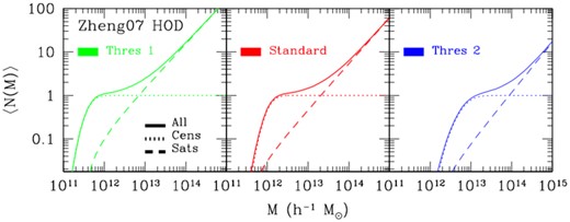
HOD shapes in the Zheng, Coil & Zehavi (2007) model, used for the production of galaxy mocks. In the various panels, dotted lines describe the central occupation statistics (equation 2), dashed lines are used for the satellite occupation statistics (equation 3), and solid lines represent the composite HODs. Three luminosity thresholds are considered, corresponding to different HOD parameter choices, as reported in Table 1. See the main text for more details.
3.3 Adding the SHMR complexity: Leauthaud model
HOD parameters for central and satellite galaxies assumed for the calibration of the Leauthaud et al. (2011) model.
| Leauthaud model | |
|---|---|
| Centrals | |
| log [M1, 0] | 12.35 |
| |$\log [M_{1 \rm a}]$| | 0.30 |
| log [M0, 0] | 10.72 |
| |$\log [M_{0 \rm a}]$| | 0.59 |
| β0 | 0.43 |
| βa | 0.18 |
| δ0 | 0.56 |
| δa | 0.18 |
| γ0 | 1.54 |
| γa | 2.52 |
| |$\sigma _{\log M_{*}}$| | 0.20 |
| Satellites | |
| αsat | 1.0 |
| βsat | 0.859 |
| Bsat | 10.62 |
| βcut | −0.13 |
| Bcut | 1.47 |
The top panel of Fig. 2 provides an example of the effects of varying in turn the five main parameters that control the SHMF (equation 5) at z = 0 by 10 per cent and up to 50 per cent – as specified in the plot with different line styles and colours, when the lognormal scatter is kept constant. The baseline parameters are fixed as in Behroozi et al. (2010) at z = 0 (solid black line, and upper part in Table 2). The bottom panel of the same figure displays the SHMF underlying the Leauthaud model at z = 0, along with its redshift evolution for the two main redshift snapshots considered in our mock-making procedure (z = 0.695 and z = 0.865, respectively – see Section 4): we use these SHMRs in our modelling.
![[Top] Effects of varying the main parameters controlling the SHMF for central galaxies (equation 5), modelled as a mean–log relation in the Leauthaud model and heavily based on Behroozi, Conroy & Wechsler (2010). The key shape parameters are altered in turn by $10{{\ \rm per\ cent}}$ (M0, M1), $20{{\ \rm per\ cent}}$ (β, δ), and $50{{\ \rm per\ cent}}$ (γ), respectively, from the baseline Behroozi et al. (2010) model at z = 0 (solid black line and upper part in Table 2), when $\sigma _{\log \rm M_{*}}=0.20$. Different line styles and colors refer to such variations, as clearly indicated in the panel. [Bottom] SHMF underlying the Leauthaud model at z = 0, and its redshift evolution at z = 0.695 and z = 0.865: we use these SHMRs in our mock-making procedure.](https://oup.silverchair-cdn.com/oup/backfile/Content_public/Journal/mnras/505/1/10.1093_mnras_staa3955/1/m_staa3955fig2.jpeg?Expires=1750312678&Signature=hWKACFYDkoCmSzKlzbNit-KczZtFyVoV04X2dXa4tB58hx41HJNuuiyXRlnaQf55CyF-YfGMtuKtlzXWOm9gbJP3S47SaL-kT8kdU2-Z6S8pqhPudLIU5jqfyFvlMst-U7-vaRlnCAFAjc7T2y5fMahr6YoDWnZu9c3sP3JWfrOpVPKHnEUklXILTEZYnySE-lUNv7QUAalFqRSR3okuNZiQJozP-xwiQ8Tmksr5erw8oY248fbVCas6-r~9iG1aJw0rOG-g4mmkF4N9JFMMVMDTd0tgBPygQTfm7IlbU9TFYbJgO7cJ793-KPH37TWbb7BRjjZOuLHuD0h5wlTZQw__&Key-Pair-Id=APKAIE5G5CRDK6RD3PGA)
[Top] Effects of varying the main parameters controlling the SHMF for central galaxies (equation 5), modelled as a mean–log relation in the Leauthaud model and heavily based on Behroozi, Conroy & Wechsler (2010). The key shape parameters are altered in turn by |$10{{\ \rm per\ cent}}$| (M0, M1), |$20{{\ \rm per\ cent}}$| (β, δ), and |$50{{\ \rm per\ cent}}$| (γ), respectively, from the baseline Behroozi et al. (2010) model at z = 0 (solid black line and upper part in Table 2), when |$\sigma _{\log \rm M_{*}}=0.20$|. Different line styles and colors refer to such variations, as clearly indicated in the panel. [Bottom] SHMF underlying the Leauthaud model at z = 0, and its redshift evolution at z = 0.695 and z = 0.865: we use these SHMRs in our mock-making procedure.
In summary, the Leauthaud framework is completely determined by 11 HOD parameters: six controlling the central galaxies and five for satellite galaxies, plus additional five if we also take into account the redshift evolution of the SHMR. In this framework, ‘threshold’ should be intended as the minimal stellar mass of the galaxy sample, rather than galaxy luminosity.
The shapes of the HODs in the Leauthaud model adopted in this work are shown in the top panels of Fig. 4 for three thresholds in mass, indicated as ‘Threshold 1’ (Th1; |$M^{\rm thr}_{*}=10^{10} \, h^{-1} \, \mathrm{M}_{\odot }$|), ‘Standard’ (Std; |$M^{\rm thr}_{*}=10^{10.5} \, h^{-1} \, \mathrm{M}_{\odot }$|), and ‘Threshold 2’ (Th2; |$M^{\rm thr}_{*}=10^{11} \, h^{-1} \, \mathrm{M}_{\odot }$|), when z = 0.695. In particular, Th2 is the one closer to the eBOSS LRG sample, and we mainly focus on this mass interval in our analysis. Note finally that in the Leauthaud framework |$\langle N_{\rm sat} (M_{\rm h} | M_{*}^{\rm thr}) \rangle$| depends on |$\langle N_{\rm cen} (M_{\rm h} | M_{*}^{\rm thr}) \rangle$|, indicating that in this particular model the occupation statistics of centrals and satellites are correlated: this constitutes an important difference with respect to the traditional five-parameter HOD. In fact, as pointed out by Contreras et al. (2017) and Duan & Eisenstein (2019), if the goal is not to constrain HOD parameters and this fitting difficulty is not of concern (as in our specific case), there is no advantage or motivation for insisting on no correlations between centrals and satellites.
3.4 HOD with colour/SFR: Tinker model
Fig. 3 shows the SHMFs adopted in the Tinker model, as well as in our mock-making procedure, along with their redshift evolution: solid lines refer to z = 0, dotted and dashed lines are at z = 0.695 and z = 0.865, respectively. Active galaxies are represented in blue, while quiescent galaxies are displayed in brown.
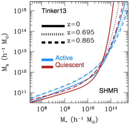
SHMFs for central galaxies adopted in the Tinker model and in our mock-making procedure at z = 0 (solid lines), z = 0.695 (dotted lines), and z = 0.865 (dashed lines). Active galaxies are displayed in blue, while quiescent galaxies are represented in brown.
As the Tinker model inherits almost all the features and methods of the Leauthaud framework, the HOD for centrals is the same as in equation (12), but the parameters of the fSHMR are independent for each subsample: this is indeed an important aspect that clearly differentiates the two models. Moreover, for red central galaxies, the HOD is multiplied by fq(Mh), and by 1 − fq(Mh) for SF central galaxies.
In summary, the Tinker model is characterized by 27 free parameters: 11 are needed for the composite HOD of a given subsample (5 for the central SHMR, one additional for the SHMR scatter, plus 5 for the satellite occupation statistics), and 5 pivot points are necessary to specify fq(Mh). Each set of 27 parameters describes the galaxy–halo relation at a given redshift, and clearly additional quantities are required to characterize the redshift evolution. In this work, we adopt literature values from the lowest redshift bin in table 2 of Tinker et al. (2013), as reported in Table 3; we note that adopting these parameters makes the model differing from that of Leauthaud, even when the full HOD shape is considered.
HOD parameters for central and satellite galaxies assumed for the calibration of the Tinker et al. (2013) model.
| TINKER MODEL | |
|---|---|
| Centrals | |
| |$\log [M_{1,0, \rm active}]$| | 12.56 |
| |$\log [M_{1,0, \rm quiescent}]$| | 12.08 |
| |$\log [M_{0,0, \rm active}]$| | 10.96 |
| |$\log [M_{0, 0, \rm quiescent}]$| | 10.70 |
| |$\beta _{0, \rm active}$| | 0.44 |
| |$\beta _{0, \rm quiescent}$| | 0.32 |
| |$\delta _{0, \rm active}$| | 0.52 |
| |$\delta _{0, \rm quiescent}$| | 0.93 |
| |$\gamma _{0, \rm active}$| | 1.48 |
| |$\gamma _{0, \rm quiescent}$| | 0.81 |
| |$\sigma _{\log \rm M_{*}, active}$| | 0.21 |
| |$\sigma _{\log \rm M_{*}, quiescent}$| | 0.28 |
| Satellites | |
| αsat, active | 0.99 |
| αsat, quiescent | 1.08 |
| βsat, active | 1.05 |
| βsat, quiescent | 0.62 |
| Bsat, active | 33.96 |
| Bsat, quiescent | 17.90 |
| βcut, active | 0.77 |
| βcut, quiescent | −0.12 |
| Bcut, active | 0.28 |
| Bcut, quiescent | 21.42 |
The central panels of Fig. 4 show the shapes of the HODs in the Tinker model adopted in this work at z = 0.695, for the same three thresholds in mass described before in relation to the Leauthaud framework, and also distinguishing between centrals and satellites. Active and quiescent galaxy HODs are represented by different colours, as indicated in the panels, and the global HODs are also displayed. As noted by Tinker et al. (2013) and also evident from our figures, the number of quiescent satellites exhibits minimal redshift evolution; all evolution in the red sequence is due to low-mass central galaxies being quenched of their star formation. Moreover, the efficiency of quenching star formation for centrals increases with cosmic time, while the mechanisms that quench the star formation of satellite galaxies in groups and clusters is losing efficiency.
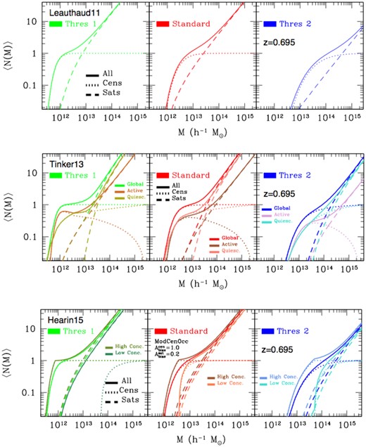
HOD shapes adopted in our mock-making procedure, at z = 0.695, for three thresholds in mass, denoted as ‘Thres 1’ (|$M^{\rm thr}_{*}=10^{10} \, h^{-1} \, \mathrm{M}_{\odot }$|), ‘Standard’ (|$M^{\rm thr}_{*}=10^{10.5} \, h^{-1} \, \mathrm{M}_{\odot }$|), and ‘Thres 2’ (|$M^{\rm thr}_{*}=10^{11} \, h^{-1} \, \mathrm{M}_{\odot }$|). Top panels display the various HODs in the Leauthaud model. Central panels show the Tinker model, where active and quiescent galaxy HODs are represented by different colours, as indicated in the figure. Bottom panels are for the Hearin HODs, where galaxies are split into upper- and lower-percentiles in terms of halo concentration, respectively, with different assembly bias strength for centrals and satellites (|$A_{\rm bias}^{\rm cen} =1.0$| and |$A_{\rm bias}^{\rm sat}=0.2$|). In all the plots, the central occupation statistics is displayed with dotted lines, the satellite occupation statistics with dashed lines, and the global HOD shapes with solid lines.
3.5 Decorated HOD: Hearin model
The fourth galaxy–halo prescription we consider is the Hearin model (Hearin et al. 2016), a decorated HOD framework designed to account for galaxy assembly bias, that naturally extends the standard HOD approach, minimally expands the parameter space, and maximizes the independence between traditional and novel HOD parameters. Galaxy assembly bias, namely the correlation between galaxy properties and halo properties at fixed halo mass, is a challenging and yet important ingredient in the galaxy–halo connection framework. The model builds on early work by Wechsler et al. (2006). The halo occupation statistics are described in terms of two halo properties rather than just one, and the extra degree of freedom has relevant impact on galaxy clustering. The formalism of the model is general and flexible, with parametric freedom, and it can be applied to any halo property in addition to halo mass; it is also readily extendable to describe HODs that depend upon numerous additional halo properties. Interestingly, the decorated HOD formalism allows one to characterize and quantify the degree of central–satellite correlation at fixed halo mass, which is an indication of compelling astrophysics – such as galactic cannibalism or conformity. We refer the reader to Hearin et al. (2016) for extensive modelling details, and report here only a few key aspects relevant to our work – see also, e.g. Xu, Zehavi & Contreras (2020) and Xu & Zheng (2020) for recent studies.
In particular, the core idea is based on the principle of ‘HOD conservation’, which preserves the moments of the standard HOD formalism: namely, it is required that the marginalized moments of a new decorated framework are equal to those of the standard HOD model, in order to minimize the modifications needed for assembly bias. In this regard, any model Pdec(Ng|Mh, x) with marginalized moments that satisfy the HOD conservation preserves the moments of Pstd(Ng|Mh), where Pstd is the occupation statistics of a standard HOD, Pdec is the occupation statistics of a decorated HOD model, and x represents a secondary halo property such that the HOD depends both on x and Mh, and the clustering of haloes depends upon x. Within this formalism, a standard HOD is recovered in the limiting condition that the strength of the assembly bias is zero.
For our purposes, we consider the Hearin model in its simplest formulation, by assuming two discrete halo subpopulations with different occupation statistics at fixed mass; this is essentially a perturbation of the Leauthaud et al. (2011) formalism, with the addition of assembly bias both in centrals and satellites. We choose the halo NFW concentration as the secondary halo property (x) used to modulate the assembly bias. Specifically, the first halo subpopulation (indicated as ‘type 1’ haloes) contains a fraction P1 of all haloes at fixed mass, for which |$x \gt \bar{x} (M_{\rm h})$|; the second subpopulation (‘type 2’ haloes) contains P2 = 1 − P1 of all haloes at fixed mass, for which |$x \lt \bar{x} (M_{\rm h})$|. The halo population is split into the P1 percentile of highest concentration haloes, and assigned a satellite galaxy occupation enhancement, while the remaining P2 = 1 − P1 percentile of lowest concentration haloes receive a satellite galaxy occupation decrement. Essentially, we require haloes at fixed mass above- or below-average concentration to have above- or below-average mean occupation. For simplicity, we assume a 50/50 split at each halo mass based on the conditional secondary percentiles: haloes within the top 50 per cent of concentration at fixed Mh are assigned to the first subpopulation, and the remaining to the second population (so P1 = P2 = 0.5). The strength of assembly bias in the occupation statistics of centrals and satellite galaxies is modulated with two free parameters |$A_{\rm bias}^{\rm cen}$| and |$A_{\rm bias}^{\rm sat}$|, respectively, where |$-1 \le A_{\rm bias}^{\rm cen} \le 1$| and |$-1 \le A_{\rm bias}^{\rm sat} \le 1$|. With this choice, a positive value for Abias implies that haloes with above-average concentration have boosted galaxy occupations; note also that more positive values of Abias correspond to models in which more concentrated haloes host more galaxies relative to less concentrated haloes of the same mass. When both of these parameters are set to zero, the model is formally equivalent to the baseline ‘no assembly bias model’ of Leauthaud et al. (2011). We consider a constant assembly bias strength at all masses for simplicity, and the sign convention is to choose type-1 haloes in the upper percentile of the secondary property. Moreover, we assume that both Pstd(Nsat|Mh) and Pdec(Nsat|Mh, x) are Poisson distributions, so that the decorated HOD is entirely specified by |$A_{\rm bias}^{\rm cen}$| and |$A_{\rm bias}^{\rm sat}$|.
In our mock-making procedure, we consider two cases for the strength of assembly bias related to centrals and satellites: in the first case (more conservative), we simply set |$A_{\rm bias}^{\rm cen} = A_{\rm bias}^{\rm sat}=0.5$|, namely the strength of assembly bias is equal for both centrals and satellites, with the boost to their mean occupation equal to 50 per cent of the maximum allowable strength at each mass; in the second case (less conservative), we set different assembly bias strengths for centrals and satellites, namely |$A_{\rm bias}^{\rm cen} =1.0$| and |$A_{\rm bias}^{\rm sat}=0.2$|. This latter choice is shown in the lower panels of Fig. 4, where we display the shapes of the Hearin HODs for the upper- and lower-percentile split in halo concentration, respectively, as indicated in the plot. In this case, the satellite HODs are also modulated by their corresponding central distributions. The same three thresholds in mass described before for the Leauthaud framework are adopted, at z = 0.695, and as usual we display the central occupation statistics (dotted lines), satellite occupation statistics (dashed lines), as well as the global HOD shapes (solid lines).
As noted by Hearin et al. (2016, 2017) and Tinker et al. (2019), assembly bias can enhance or diminish the clustering on large scales, but in general it increases the clustering on scales below Mpc – being qualitatively different at large and small scales. Also, assembly bias in satellites versus centrals imprints a distinct signature on galaxy clustering as well as lensing, and the degree to which assembly bias alters galaxy clustering statistics can be quite sensitive to the underlying baseline mass-only HOD of the galaxy population under consideration. In particular, the impact of assembly bias on galaxy clustering is quite sensitive to the steepness of the transition from 〈Ncen|Mh〉std = 0 at low host masses to 〈Ncen|Mh〉std = 1 at high host masses. This steepness is controlled by the level of stochasticity in the central galaxy stellar mass at fixed halo mass, parametrized in our baseline model by |$\sigma _{\log \rm M_{*}}$|. Note that changing the values of Abias does not change 〈Ng|Mh〉, the mean number of galaxies averaged over all haloes of fixed mass: this is the defining feature of the decorated HOD, and the meaning of the principle of HOD conservation.
4 MODELLING THE GALAXY–HALO CONNECTION: TOOLS AND METHODOLOGY
In this section, we briefly describe the tools and methodologies behind our mock-making procedure, the main N-body simulation used, and the pipeline to produce novel heterogeneous sets of Outer Rim-based galaxy catalogues.
4.1 Outer Rim mocks
The baseline simulation used for all our mock-making procedure is the Outer Rim (OR) run, extensively described in Heitmann et al. (2019). The simulation has been developed along the glorious tradition of the Millennium simulation (Springel 2005), with similar mass resolution but a volume coverage increase by more than a factor of 200. Currently, the Outer Rim is among the largest high-resolution gravity-only N-body simulations ever performed, spanning a (|$3 \, h^{-1}\, {\rm Gpc})^3$| volume, and characterized by an unprecedented combination of volume and mass resolution (down to |$1.85 \times 10^9 \, h^{-1} \, \mathrm{M}_{\odot }$|) evolving 1.07 trillion particles – i.e. 102403. The actual size of the simulation was chosen to cover a volume large enough to enable synthetic sky catalogues for eBOSS, DESI, and LSST, while maintaining adequate mass resolution to capture haloes reliably down to small masses. The entire run was carried out at the Argonne Leadership Computing Facility on Mira, a Blue-Gene/Q many-core supercomputer. The simulation code adopted is an optimized version of the Hardware/Hybrid Accelerated Cosmology Code (hacc), designed to overcome numerical challenges; see Habib et al. (2016) for all the details. The cosmology of the simulation is close to the best-fittingWMAP-7 fiducial model (Komatsu et al. 2011), namely ωc = 0.1109, ωb = 0.02258, ns = 0.963, h = 0.71, σ8 = 0.8, w = −1, with no massive neutrinos (Ων = 0) and assuming flatness. The dynamical range of the simulation is remarkable, spanning 106 orders of magnitudes, with a force resolution of |$6h^{-1}\, {\rm kpc}$|. Initial conditions are fixed at zin = 200 with the Zel’dovich approximation (Zel’dovich 1970). Transfer functions are generated via camb (Lewis, Challinor & Lasenby 2000).
A total of 101 redshifts in output were originally saved, from z = 10 to z = 0, evenly spaced in log a, with a the scale factor. In our study, we mainly focus on 2 redshift intervals, namely z = 0.695 and z = 0.865, although we also consider a variety of other redshifts from some of the realizations to assess redshift evolution. Each snapshot encompasses globally about 40TB of data, and the entire data volume of the simulation is more than 5PB; all particle information for haloes with more than 100 000 particles is stored for substructures and shape studies, as well as a random selection of 1 per cent of particles in each halo (with a minimum of five particles per halo).
For our mock-making purposes, we had access to the friends-of-friends (FOF) halo catalogue at various redshifts, generated using a linking length b = 0.168.5 Haloes are defined by more than 20 particles, and found with a customized FOF finder (Woodring et al. 2011; Heitmann et al. 2019) that follows the standard implementation, having the linking length defined with respect to the mean interparticle spacing. All the centres of the haloes are determined by the location of the FOF halo’s minimum gravitational potential, and the centre-of-mass and the halo velocities are obtained by summing over all positions and velocities and dividing by the number of particles. The FOF halo mass is simply determined by the number count of particles in each halo.
For a given redshift, our halo catalogue (split into 110 subfiles, stored in a way such that they are not contiguous volumes) contains the number of particles in halo (Halo Count), the halo ID (Halo Tag), the halo FOF mass in |$h^{-1}\, {\rm M}_{\odot }$| units, the comoving halo centre positions from the potential minimum (in |$h^{-1}\, {\rm Mpc}$|), and the comoving peculiar velocities of halo centres (in km s−1). Note that the halo centre is defined by its potential minimum most bound particle, since accurate centre-finding is important for measuring the halo concentration, for halo stacking, and for placing central galaxies from HOD modelling.
Fig. 5 visualizes a small portion of the Outer Rim halo catalogue at z = 0.865. Specifically, the left-hand panel shows a |$100 \times 100 ~[h^{-1} \, {\rm Mpc}]^2$| projection along x and y and across z, having thickness |$\Delta z=50~h^{-1} \, {\rm Mpc}$|; points in the figure are FOF haloes, colour coded by their mass. The middle panel is a progressive zoom into a |$50 \times 50 ~[h^{-1} \, {\rm Mpc}]^2$| block having the same depth as the left one, while the right-hand panel shows an individual halo of mass |$4.938 \times 10^{13}~h^{-1}\, {\rm M_{\odot }}$| rendered with 1 per cent of random particles, located inside the smaller |$7 \times 7~[h^{-1} \, {\rm Mpc}]^2$| white inset: it is possible to appreciate the neat ellipsoidal halo shape. Length units displayed in the left-hand panel are in |$h^{-1} \, {\rm Mpc}$|. The high resolution of the simulation, down to |$1.85 \times 10^9 \, h^{-1} \, \mathrm{M}_{\odot }$|, allows one to resolve accurately also relatively low-mass haloes.
![Small portion of the Outer Rim halo catalogue at z = 0.865. The left-hand panel is a $100 \times 100 ~[h^{-1} \, {\rm Mpc}]^2$ projection along x and y and across z, with thickness $\Delta z=50~h^{-1} \, {\rm Mpc}$, while the middle panel is a progressive zoom into a $50 \times 50 ~[h^{-1} \, {\rm Mpc}]^2$ block. Points the figure are FOF haloes, colour coded by their mass. Zooming into a smaller $7 \times 7~[h^{-1} \, {\rm Mpc}]^2$ inset of the halo catalogue, the right-hand panel displays the ellipsoidal shape of a halo of mass $4.938 \times 10^{13}~h^{-1}\, {\rm M_{\odot }}$ contained inside that area, rendered with a 1 per cent random particle subsample. Length units displayed in the left-hand panel are in $h^{-1} \, {\rm Mpc}$. The high resolution of the simulation, down to $1.85 \times 10^9 \, h^{-1} \, {\rm M_{\odot }}$, allows one to resolve accurately also relatively low-mass haloes.](https://oup.silverchair-cdn.com/oup/backfile/Content_public/Journal/mnras/505/1/10.1093_mnras_staa3955/1/m_staa3955fig5.jpeg?Expires=1750312678&Signature=Gcf-2~xPMPhVK92j0-hwcpWWj0HERD0h4VTKq1Gufk2GKZTn~9KxSfk8d4aQvarF1Kk-3HsCAEU50XTTPO5GcWPPo6Cs4VM~a2tO~ZaET2KSw2oHOAvno1j8NesVb0CFsW7M-N8L37BsnV6~W9zi1J95JaXAX8bsZsLCeqtQ-bfMU8eoeoq0QHmZ3Cg7hX3c9nPOdCHRAqzRNdB1BS4h2h5Zj36SU-8fIfTH8MtmrbEk-F30rP9Gw3qSixshS0soos~t7RBd8tbQlop9IbI0S2tDEOZNisE6IwHui1shq08QjvxKCUlWxs3XlGXmTiZUbudvEnbjXUBNVxnRLx2g2A__&Key-Pair-Id=APKAIE5G5CRDK6RD3PGA)
Small portion of the Outer Rim halo catalogue at z = 0.865. The left-hand panel is a |$100 \times 100 ~[h^{-1} \, {\rm Mpc}]^2$| projection along x and y and across z, with thickness |$\Delta z=50~h^{-1} \, {\rm Mpc}$|, while the middle panel is a progressive zoom into a |$50 \times 50 ~[h^{-1} \, {\rm Mpc}]^2$| block. Points the figure are FOF haloes, colour coded by their mass. Zooming into a smaller |$7 \times 7~[h^{-1} \, {\rm Mpc}]^2$| inset of the halo catalogue, the right-hand panel displays the ellipsoidal shape of a halo of mass |$4.938 \times 10^{13}~h^{-1}\, {\rm M_{\odot }}$| contained inside that area, rendered with a 1 per cent random particle subsample. Length units displayed in the left-hand panel are in |$h^{-1} \, {\rm Mpc}$|. The high resolution of the simulation, down to |$1.85 \times 10^9 \, h^{-1} \, {\rm M_{\odot }}$|, allows one to resolve accurately also relatively low-mass haloes.
4.2 nseries mocks
In addition to the heterogeneous sets of high-fidelity Outer Rim mocks developed in this work, we also exploit a small homogeneous set indicated as the nseries, which has been previously used in the SDSS DR12 galaxy clustering analysis (Alam et al. 2017). The homogeneous set, comprised of 84 mocks in total, is particularly suitable to address cosmic variance and modelling systematics at the sub-per cent level, since all mocks have the same underlying galaxy bias model built upon the same cosmology, but each mock is a quasi-independent realization – thus not sharing the same LSS. Moreover, these mocks are cut sky: they have the same angular and radial selection function as the NGC DR12 CMASS sample within the redshift range 0.43 < z < 0.70, and therefore they include observational artefacts closer to the eBOSS DR16 sample. The N-body simulations from which these cut-sky mocks were created have been produced with gadget2 (Springel 2005), with input parameters to ensure sufficient mass and spatial resolution to resolve the haloes that BOSS galaxies occupy. Specifically, the nseries cosmology is characterized by Ωm = 0.286, h = 0.7, Ωb = 0.047, σ8 = 0.820, and ns = 0.96. The main difference with respect to the Outer Rim mocks – apart from being cut sky and not built on periodic cubes – is that the nseries derive from multiple realizations of the dark matter field on a larger volume with different random seeds (i.e. a series of N-body simulations identical in all but in the initial random seed), which allows one to address the impact of cosmic variance: this is not achievable with only a halo catalogue nor a single N-body simulation at hands.
4.3 EZMOCKS
For determining the rescaled covariance matrices functional to the subsequent analyses, we also make use of a new series of DR16 ezmocks, thoroughly described in Zhao et al. (2020). These large number of galaxy catalogues (1000 per tracer), having accurate clustering properties, are generated with a complex methodology built around the Zel’dovich approximation (Zel’dovich 1970), and effectively including stochastic scale-dependent, non-local, and non-linear biasing contributions; extensive details on the methodology can be found in the first release paper by Chuang et al. (2015). Non-local effects, such as tidal fields not included in linear Lagrangian Perturbation Theory (LPT) or other biasing contributions, are effectively included in both the scatter relation and the tilting of the initial power spectrum. The missing power towards small scales of perturbative approaches is included in the modulation of the initial power spectrum, when fitting for the resulting halo populations. These mocks have accurate clustering properties – nearly indistinguishable from full N-body solutions – in terms of the one-point, two-point, and three-point statistics. The underlying cosmology is based on a flat ΛCDM model, with Ωm = 0.307115, Ωb = 0.048206, h = 0.6777, σ8 = 0.8225, and ns = 0.9611. Specifically for LRGs, they contain the complexity of blending the CMASS plus eBOSS LRG samples, as well as all the realistic effects of mask, cut sky, and observational systematics (i.e. fibre completeness, spectroscopic success rate, redshift failures, photometric systematics). For our analysis, we adopt dedicated cubic ezmocks rather than the cut sky set for covariance estimations, to comply with the characteristics of the high-fidelity Outer Rim-based realizations. The ezmocks are extensively used in all the supporting eBOSS DR16 papers and in the final eBOSS consensus analysis. For additional technical details, we refer the reader to the companion paper by Zhao et al. (2020).
4.4 Galaxy mock-making procedure: methods
Our synthetic high-fidelity galaxy mocks are primarily produced exploiting the standard halotools6 framework (Hearin et al. 2017), and by introducing a number of customizations depending on the desired challenge and model explored (see Section 6, as well as the previous theoretical part). In particular, we interface halotools capabilities with the Outer Rim halo catalogue at different redshifts. halotools is an open-source, community-driven Python powerful package for studying the galaxy–halo connection, which provides a highly modular, object-oriented platform for building HOD models, so that individual modelling features can easily be swapped in and out. This modularity facilitates rigorous study of all the components that makes up a halo occupation model, and has been designed from the ground-up with assembly bias applications in mind. In this view, although our main products are based on the Outer Rim simulation, following the halotools philosophy the pipelines developed here are written in a general and flexible manner, so that any type of customization is readily achievable with minimal efforts and modifications; hence, our modular approach procedure is quite general, and readily applicable to any halo catalogue and survey design in mind. The concept of generality and reusability of the code is in fact what has driven this design from the start. In this view, although we limit here our modelling approach to HOD-based techniques (mainly due to limitations in our available halo catalogue products), we plan to pursue subhalo and abundance matching methods in follow-up studies, using the same code and modular structure.
Adopting halotools conventions, three main primary keyword arguments are used to customize all the instances retrieved by the mock factory, common to all the different HOD models developed here (besides specific HOD parameters), namely: redshift, threshold, and modulate_with_cenocc – the latter being the modulation of the satellite distribution with the central one. In our mock-making procedure, except for the Hearin framework, all other satellite HODs are not modulated by their corresponding central distributions. Also, as previously mentioned, we treat the conventional Zheng model separately since its HOD is effectively redshift-independent and the meaning of ‘threshold’ in the model is based on luminosity rather than stellar mass, unlike for the other three frameworks considered (i.e. Leauthaud, Tinker, Hearin). Specifically, halotools is used to populate dark matter haloes in the Outer Rim simulation with galaxies having a stellar mass |$M_{*} \gt 10^{10.0}~h^{-1} \, \mathrm{M}_{\odot }$| (‘Threshold 1’), |$M_{*} \gt 10^{10.5}~h^{-1} \, \mathrm{M}_{\odot }$| (‘Standard’), and |$M_{*} \gt 10^{11.0}~h^{-1} \, \mathrm{M}_{\odot }$| (‘Threshold 2’). This roughly correspond to ‘Threshold 1’ (Mr = −19), ‘Standard’ (Mr = −20), and ‘Threshold 2’ (Mr = −21), respectively, in the Zheng formalism.
All these high-fidelity mocks have been produced at the National Energy Research Scientific Computing Center (NERSC), a DOE Office of Science User Facility supported by the Office of Science of the U.S. Department of Energy, under Contract No. DE-AC02-05CH11231 using the Cori supercomputer, a Cray XC40 with a peak performance of about 30 petaflops. Cori is comprised of 2388 Intel Xeon ‘Haswell’ processor nodes, and 9688 Intel Xeon Phi ‘Knight’s Landing’ (KNL) nodes. The system also has a large Lustre scratch file system and a first-of-its kind NVRAM ‘burst buffer’ storage device. We devised new customized scripts and pipelines to produce such mocks on Cori, exploiting especially the multithread architecture. Our mock-making code/pipeline is memory efficient and optimized to the machine. Some additional supporting numerical work has also been carried out using the Korea Institute of Science and Technology Information (KISTI) supercomputing infrastructure.
In closing this part, we note that our main goal in the cubic N-body-based mock-making production and in the related mock challenge is to test the validity and robustness of different BAO and RSD fitting techniques on a common ground against a series of different HOD prescriptions, and validate the clustering analysis pipelines and the various RSD models. Hence, we are not concerned with reproducing exactly all the features of the eBOSS DR16 LRG sample, and this is why the various HOD parameters that enter in the models outlined in Section 3 have been maintained to their corresponding literature values. Nevertheless, in Section 6 we show an instructive comparison between eBOSS measurements and those obtained from Outer Rim TH2 mocks. Note also that the HOD parameters adopted from the literature were chosen under cosmologies different from that of the Outer Rim, and therefore we do not expect to find the same results as in the corresponding original publications: this is clearly not affecting the conclusions of our work. Realistic observational artefacts related to the LRG sample, such as cut sky, matching number density, observational systematics, etc., are instead part of the ezmocks release (Zhao et al. 2020).
5 ANALYSIS: METHODOLOGY
In this section, we briefly describe the three configuration and Fourier space techniques used in the analysis of the challenge mocks, based on three different RSD analytical models – exploiting the FS information in the correlation function or power spectrum. The detailed BAO modelling is instead described in our LRG companion papers. All these methods are adopted in the main analysis of the final eBOSS DR16 LRG sample.
5.1 CLPT-GS
With this technique, the FS RSD analysis in configuration space is performed, and for a given cosmology the model has four free parameters, namely (fσ8, F′, F″, σFOG), with f the linear growth factor and F′ and F″ the first and second derivatives of the Lagrangian bias function F. For extensive details on this method see Bautista et al. (2020) and Icaza-Lizaola et al. (2020).
5.2 TNS in configuration space
The linear and non-linear matter power spectra entering in the model are computed with camb and the halofit semi-analytical prescription, respectively. To obtain Pθθ and Pδθ, we use the universal fitting functions provided by Bel et al. (2019). In particular, the overall degree of non-linear evolution is encoded via the amplitude of the matter fluctuation at the effective redshift considered. Finally, the multipole moments of the anisotropic correlation function are obtained by performing the Hankel transform of the model, and regarding the RSD part, the implementation of the AP effect follows the formalism of Xu et al. (2013): the AP distortions are modelled through the α and ϵ parameters, which characterize the isotropic and anisotropic distortion components, respectively.
With this technique, the FS RSD analysis in configuration space is performed, and for a given cosmology the model has five free parameters, namely (f, σ8, b1, b2, σv) – although since f and σ8 are degenerate they are thus combined at the level of the likelihood into the single parameter fσ8. For extensive details on this method see de la Torre et al. (2017), Mohammad et al. (2018), and Bautista et al. (2020).
5.3 TNS in Fourier space
While the previous techniques are used to carry out the analysis of the LRG sample in configuration space, the method described here – also based on the TNS model and indicated as ‘Pk-TNS’ – is performed in Fourier space. To this end, the modelling of the BAO signal within this framework – along with the BAO fitting procedure in Fourier space – are described in Gil-Marín et al. (2020). Here, we briefly illustrate only the strategy adopted for the RSD and AP analysis, exploiting the FS information in the power spectrum.
With this technique, the FS RSD analysis in Fourier space is performed, and for a given cosmology the model has seven free parameters, namely (α∥, α⊥, fσ8) and (b1, b2, Anoise, σFoG). Note that while the BAO analysis consists of using a fixed and arbitrary template to compare the relative BAO-peak positions in the power spectrum multipoles, the FS analysis allows for a full modelling of the shape and amplitude of the power spectrum multipoles, taking into account DM non-linear effects, galaxy bias, and RSDs. For extensive details on this method see Gil-Marín et al. (2020).
6 THE GALAXY MOCK CHALLENGE
In this section, we present the main outcomes of the galaxy mock challenge. After a brief description of the mock products directly useful in the actual fits considered in the HOD systematic error budget, we show selected results in configuration and Fourier space. We eventually compare the complementary BAO/RSD models adopted for the analysis of the complete DR16 eBOSS LRG sample, assessing the theoretical systematic budget. Our findings demonstrate that all the methods are mutually consistent, with comparable systematic errors on the AP parameters and the growth of structures, and robust to different HOD prescriptions – thus validating the clustering analysis pipelines.
6.1 Mock products used in the analysis
For the galaxy mock challenge, we devised three sets of heterogeneous Outer Rim-based galaxy mocks (indicated as ‘Challenge Set 1’, ‘Challenge Set 2’, ‘Challenge Set 3’, respectively).7 These are cubic mocks, in the Outer Rim cosmology, obtained by populating Outer Rim halo catalogues with galaxies using the Zheng, Leauthaud, Tinker, and Hearin HOD prescriptions – as explained in Section 4.1. Extensive details regarding each set are provided in Appendix A. For the main analysis presented here, focused on testing the BAO templates and the RSD models adopted for the characterization of LRG clustering systematics, we only use a subset of those mocks drawn from ‘Challenge Set 1’ at z = 0.695 assuming the ‘Threshold 2’ (Th2) flavour. As explained in Sections 3 and 4.4, the meaning of ‘flavour’ is related to the halotools key parameter ‘threshold’, which globally sets all the individual HOD parameters as best-fitting realizations from the corresponding literature dictionary of each HOD model (unless customizations are introduced). Specifically, we select Th2 mocks with the Leauthaud, Tinker, and Hearin prescriptions, respectively, since their number density is closer to the eBOSS LRG sample (see Table A2). Moreover, since we require fully independent mocks (i.e. not sharing the same DM field), we only consider 27 realizations per HOD per flavour: such realizations are obtained by populating once the full |$3 \, h^{-1} \, {\rm Gpc}$| Outer Rim periodic halo catalogue box with galaxies, and then by cutting the full box into 27 non-overlapping subcubes of |$1h^{-1}\, {\rm Gpc}$| side and rescaling the various spatial positions accordingly. In fact, by construction, at a fixed z and for a fixed set of HOD parameters, the central galaxies will always reside at the centre of their hosted haloes, inheriting the same halo velocity; hence, additional subcubes would be fully or highly correlated in the central galaxy population, depending on how the box is cut. We then add RSDs to each individual mock in two different ways: radially, or with the usual plane-parallel approximation.
In Fig. 6, we show an example on how satellite galaxies are distributed within the same Outer Rim halo, according to the different HOD prescriptions presented in Section 3, to convey some intuition on the galaxy–halo connection modelling and the spatial location of satellites. The plot displays the x–y spatial projection at z = 0.695 of a randomly chosen halo, with its spherical shape determined by its virial radius. The standard Zheng model is shown in the upper left-hand panel, and clockwise the Leauthaud, Hearin, and Tinker models are displayed, respectively. While in all the HOD schemes the satellite phase space statistics follow an unbiased NFW profile with a phase space distribution in isotropic Jeans equilibrium and galaxy concentration identical to that of the parent halo, more sophisticated frameworks such as the Tinker model (lower left corner) are able to distinguish between active and quiescent populations (indicated with different colours in the panel), thus providing additional useful physical insights.
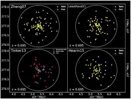
Example of the distribution of satellite galaxies within the same and randomly chosen Outer Rim halo, at z = 0.695, according to the different HOD prescriptions presented in Section 3. The plot represents a spatial projection (x − y) of the halo, and its spherical shape as determined by its virial radius is also indicated in the various panels. Clockwise, starting from the upper left corner, the Zheng, Leauthaud, Hearin, and Tinker models are shown, respectively.
Moreover, in addition to the heterogeneous Outer Rim mocks, as detailed in Section 4.2 we also exploit 84 homogeneous cut-sky nseries mocks, which have been previously used in the SDSS DR12 galaxy clustering analysis (Alam et al. 2017), to address cosmic variance in the various methods – since the nseries derive from multiple realizations of the dark matter field with different random seeds. Here we show only one global nseries application, while in Gil-Marín et al. (2020) and Bautista et al. (2020) those mocks are extensively used to assess systematics related to each individual fitting method in configuration or Fourier space, respectively.
6.2 Galaxy mock challenge: BAO analysis and HOD systematics
Approximate catalogues such as the ezmocks (Zhao et al. 2020) are in principle sufficient for covariance estimates and for quantifying systematic biases in BAO studies, while the analysis of the FS of the correlation function and power spectrum requires high-fidelity (N-body-based) mocks to precisely test the modelling. Nevertheless, using high-resolution mocks, we are able to characterize the impact of systematics in HOD modelling both on BAO and RSD constraints with high-accuracy. Specifically, the main goals are to quantify possible effects induced by different galaxy HOD schemes on the cosmic growth rate and obtain useful information on parameter inference based on HOD variations, to assess the impact of an arbitrary choice of the BAO reference template on the inferred cosmological parameters, and more generally to determine the theoretical systematic budget and validate the clustering analysis pipelines.
The standard procedure common to all BAO fitting methods is to assume a fixed and arbitrary template, and compare the relative BAO peak positions in the correlation function or power spectrum multipoles. Reconstruction techniques such as those presented in Burden et al. (2014), Burden, Percival & Howlett (2015) are then applied to the density field, in order to remove a fraction of the RSDs and the non-linear motions of galaxies. The BAO feature in the 2-point statistics (both in configuration and Fourier space) is sharpened, increasing the precision of the measurement of the acoustic scale.
The BAO scale measurement in configuration space adopted here is the same as the one described in previous SDSS publications (i.e. Alam et al. 2017; Ata et al. 2018; Bautista et al. 2018), and thoroughly illustrated in our companion paper Bautista et al. (2020), while the modelling of the BAO signal along with the BAO fitting procedure in Fourier space are explained in detail in Gil-Marín et al. (2020). In particular, for the latter case, the power spectrum anisotropic signal is modelled in order to measure the BAO peak position and marginalize over the broad-band information – taking into account the BAO signal both in the radial and transverse LOS directions. Generally, BAO results are obtained from pre- and post-reconstructed data, while RSD results use only the non-reconstructed sample. In the following analyses, we assume standard dependence of the growth rate f, and adopt a smoothing scale of 15 h−1Mpc. Whenever required, galaxy redshifts are converted into radial comoving distances for clustering measurements, using the cosmological parameters of the OR simulation. As shown in Bautista et al. (2020), the analysis methodology is insensitive to the choice of a fiducial cosmology.
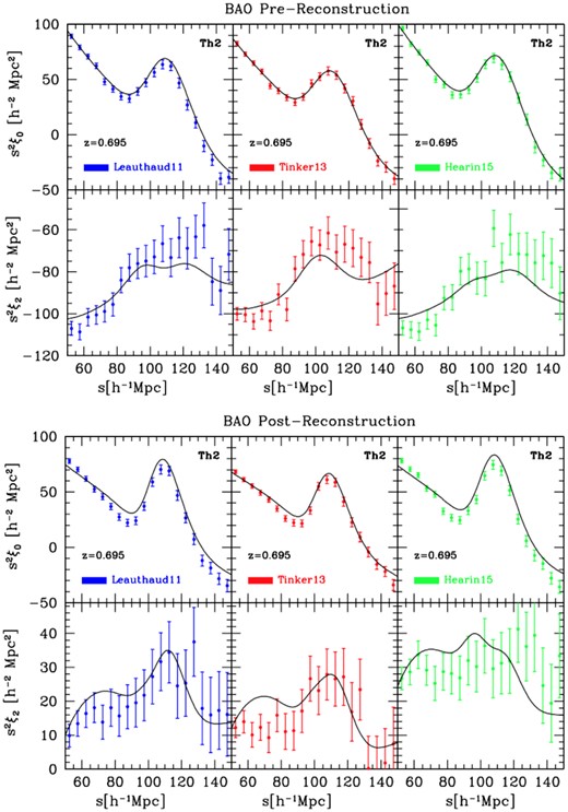
Monopole and quadrupole of the average 2PCFs as computed from a subset of 27 OR-based mocks per HOD type, and fits of the BAO feature as seen in the correlation function multipoles. Top panels show results for the pre-reconstruction case, bottom panels refer to the reconstructed density field. The HOD models of Leauthaud, Tinker, and Hearin are shown – from left to right, respectively – for the ‘Th2’ flavour at z = 0.695. Note that the BAO feature (around |$100 \, h^{-1}\, {\rm Mpc}$|) appears much sharper after application of the reconstruction procedure, as expected. Results of these fits are reported in Table 4.
BAO fits to the average pre- and post-reconstructed 2PCFs for different HOD prescriptions over 27 corresponding Outer Rim mock realizations, at z = 0.695, with the ‘Th2’ flavour – as displayed in Fig. 7.
| CF [Th2] | Leauthaud | Tinker | Hearin |
|---|---|---|---|
| BAO | Pre-Rec | ||
| α⊥ | 0.9990 ± 0.0080 | 0.9922 ± 0.0073 | 1.0074 ± 0.0083 |
| α∥ | 1.0084 ± 0.0164 | 1.0234 ± 0.0147 | 1.0040 ± 0.0157 |
| Σ⊥ | 6.7663 ± 1.1320 | 7.6741 ± 1.2932 | 7.4335 ± 1.0760 |
| Σ∥ | 10.5333 ± 1.5795 | 8.4652 ± 1.5436 | 9.5687 ± 1.6354 |
| β | 0.2685 ± 0.0965 | 0.2404 ± 0.1017 | 0.2137 ± 0.0910 |
| b | 2.6748 ± 0.1315 | 2.4769 ± 0.1393 | 2.7525 ± 0.1339 |
| χ2 | 129.4 | 115.4 | 126.0 |
| BAO | Post-Rec | ||
| α⊥ | 1.0045 ± 0.0056 | 1.0014 ± 0.0060 | 1.0066 ± 0.0057 |
| α∥ | 0.9937 ± 0.0084 | 0.9976 ± 0.0090 | 1.0115 ± 0.0094 |
| Σrec | 15.0 ± 1.5 | 15.0 ± 1.5 | 15.0 ± 1.5 |
| Σ⊥ | 2.0002 ± 11.9307 | 2.0000 ± 0.9844 | 2.9483 ± 1.3018 |
| Σ∥ | 4.0169 ± 1.6667 | 4.9272 ± 1.3161 | 6.8683 ± 1.1810 |
| β | 0.4018 ± 0.0911 | 0.5127 ± 0.0863 | 0.4157 ± 0.0849 |
| b | 2.3873 ± 0.0744 | 2.1669 ± 0.0710 | 2.5137 ± 0.0879 |
| χ2 | 131.3 | 130.0 | 164.5 |
As mentioned in Section 4.4, the OR-based mocks have not been designed to reproduce all of the features of the eBOSS DR16 LRG sample, since that level of complexity is not necessary for our subsequent analysis. Hence, we clearly do not expect to exactly match the clustering properties of the eBOSS LRG sample. Nevertheless, as an instructive example, we show in Fig. 8 a comparison between eBOSS measurements and those made from Th2 OR mocks at z = 0.695. Specifically, green triangles in the figure display eBOSS plus CMASS measurements for the NGC, pink squares are used for eBOSS plus CMASS SGC measurements, and yellow circles show results obtained from the combined samples. Open symbols refer to pre-reconstruction calculations (top panel), while filled symbols indicate post-reconstruction results (bottom panel). Errorbars are estimated from analogous measurements performed on 1000 ezmocks, and via averaging. The solid black line in both panels represents the redshift-space 2PCF monopole expectation assuming the Tinker HOD recipe, derived from 27 Th2 OR mocks. Note that, besides not tuning the various HOD parameters to reproduce the exact clustering properties of the eBOSS DR16 LRG sample, our OR-based realizations are cubic mocks, and do not contain the complications of masks, cut sky, and observational artefacts (as opposed to the ezmocks and nseries) – which would be instead more appropriate for a fair data-mock comparison.
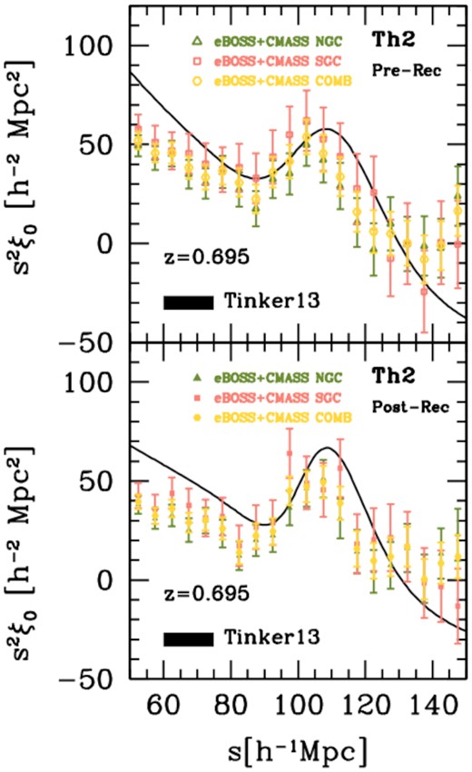
Illustrative example showing the comparison between eBOSS measurements and those made from Th2 OR mocks at z = 0.695. The top panel displays pre-reconstruction calculations (reported with open symbols), while the bottom panel refers to post-reconstruction results (indicated with filled symbols). The green triangles in the figure show eBOSS+CMASS measurements for the NGC, pink squares are used for eBOSS + CMASS SGC measurements, and yellow circles represent the combined samples. Errorbars are estimated from 1000 ezmocks. The solid black line in both panels is the redshift-space 2PCF monopole expectation assuming the Tinker HOD recipe, derived from 27 Th2 OR mocks, without including the complications of masks, cut sky, and observational artefacts.
Fig. 9 shows examples of redshift-space galaxy power spectra as computed from the average of 27 OR-based mocks, each set being characterized by a different HOD scheme, at z = 0.695 for the ‘Th2’ flavour. The plot represents the analogous, in Fourier space, of the previous correlation function estimates in configuration space. The pre- (top panels) and post-reconstructed (bottom panels) monopoles and quadrupoles of the power spectra are shown, for the Leauthaud, Tinker, and Hearin models – from left to right, respectively. Fits are obtained with the BAO theoretical model of Gil-Marín et al. (2020), considering wave numbers between 0.02 ≤ k[hMpc−1] ≤ 0.30, and the corresponding results are reported in Table 5. Unlike correlation function calculations, Discrete Fourier Transform (DFT) methods used to compute the power spectrum multipoles are quite sensitive to the assumption of periodic boundary conditions, and therefore a procedure denoted as ‘padding’ is applied in this process, to mitigate non-periodicity effects. The detailed effects of non-periodicity on BAO measurements are discussed in Gil-Marín et al. (2020). In particular, results of such analyses show that no significant changes are observed in terms of α⊥, while shifts at the level of |$2\!-\!3{{\,\rm per\,cent}}$| can be systematically seen in α∥ if padding is not applied. Hence, non-periodic effects are relevant in determining α∥, but they do not impact significantly α⊥. Moreover, no relative shifts in any of the α parameters are seen when the HOD model or flavour is varied – as we show next.
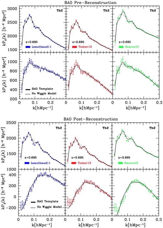
Monopole and quadrupole of the average power spectra as computed from a subset of 27 OR-based mocks per HOD type, and fits of the BAO feature as seen in the power spectrum multipoles (solid lines). The corresponding no-wiggle model is also reported in the figure, with dotted lines. Top panels show results for the pre-reconstruction case, bottom panels refer to the reconstructed density field. The HOD models of Leauthaud, Tinker, and Hearin are shown – from left to right, respectively – for the ‘Th2’ flavour at z = 0.695. Results of these fits are reported in Table 5.
BAO fits to the average pre- and post-reconstructed power spectra for different HOD prescriptions over 27 corresponding Outer Rim mock realizations, at z = 0.695, with the ‘Th2’ flavour – as displayed in Fig. 9.
| PS [Th2] | Leauthaud | Tinker | Hearin |
|---|---|---|---|
| BAO | Pre-Rec | ||
| α⊥ | 1.0028 ± 0.0107 | 0.9953 ± 0.0124 | 1.0108 ± 0.0099 |
| α∥ | 0.9885 ± 0.0178 | 1.0023 ± 0.0177 | 0.9779 ± 0.0143 |
| Σ⊥ | 4.2992 ± 1.8875 | 5.9568 ± 2.0364 | 4.1865 ± 1.8043 |
| Σ∥ | 9.6867 ± 1.8250 | 7.5044 ± 2.2301 | 7.0045 ± 2.0438 |
| χ2 | 44.3 | 34.5 | 57.8 |
| BAO | Post-Rec | ||
| α⊥ | 0.9976 ± 0.0075 | 0.9975 ± 0.0088 | 1.0122 ± 0.0075 |
| α∥ | 0.9938 ± 0.0104 | 0.9976 ± 0.0121 | 1.0002 ± 0.0113 |
| Σrec | 15.0 ± 1.5 | 15.0 ± 1.5 | 15.0 ± 1.5 |
| Σ⊥ | 1.0585 ± 0.7909 | 1.3377 ± 0.9904 | 1.1071 ± 0.8221 |
| Σ∥ | 1.5451 ± 1.1110 | 1.9511 ± 1.3408 | 2.5084 ± 1.5258 |
| χ2 | 94.4 | 69.0 | 120.1 |
Fig. 10 summarizes and confronts the performance of the BAO fitting technique adopted in the analysis of the final eBOSS LRG sample, in configuration and Fourier space, with respect of variations in the underlying HOD model. For each mock realization, at a fixed HOD scheme and threshold flavour, the correlation function and power spectrum are computed along with their multipoles, respectively. Subsequently, fits for the BAO peak position are performed – both to the pre- and post-reconstructed synthetic catalogues – to determine the dilation parameters α∥ and α⊥ and their corresponding errors. The expected values for the dilation parameters are computed in the OR cosmology, at the effective redshift |$\bar{z} =0.695$|. In addition, fits to the average multipoles of a given set of mocks (27 mocks per set) are also carried out, to probe biases in a very high precision configuration. In particular, the BAO pipeline on the power spectrum monopole and quadrupole is run in the interval 0.02 ≤ k[hMpc−1] ≤ 0.30. The various BAO fittings are performed by fixing the BAO damping parameters (Σ∥, Σ⊥) at their best-fitting values on the mean of the pre- and post-reconstructed mocks, and the analysis is done in terms of the scaling parameters α⊥ and α∥. The various covariances used in the analysis of the OR-based mocks are derived from the ezmocks, properly rescaled to account for differences in number density (see Table A2). As explained in detail in Bautista et al. (2020), the final BAO model is a combination of the cosmological multipoles ξℓ and a smooth function of separation, which accounts for unknown systematic effects in the survey that can potentially contaminate the results.
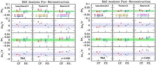
Performance of the BAO fitting methods in configuration and Fourier space, with respect of variations in the underlying HOD model. Fits to individual mock realizations as well as to the mean of a set of 27 independent realizations of the OR mocks (from the ‘Challenge Set 1’) are carried out (see Table B2). The difference between the measured α∥ and α⊥ from pre- (left-hand panels) and post-reconstructed (right-hand panels) catalogues are displayed with different symbols and colours, as indicated in the figure. This BAO fitting methodology is adopted in the analysis of the final eBOSS LRG sample. The shaded dark-green areas in the figure highlight the |$1{{\ \rm per\ cent}}$| error level, while horizontal grey bands display 1σ error levels. Overall, we do not detect any significant systematics due to different HOD prescriptions: after application of the BAO reconstruction procedure, all of the mean measurements are within |$0.5\!-\!1.2{{\ \rm per\ cent}}$| of their expected values, thus below the statistical precision of the eBOSS LRG sample. See the main text for more details.
Table B2 contains the results when fitting the mean correlation functions and power spectra (rows labelled ‘Mean’) of the 27 independent realizations of the OR-based mocks with different HOD prescriptions, as well as the mean of the fits of individual realizations (rows labelled ‘Individual’). Those data are shown in Fig. 10, where each subpanel displays the difference between the measured α∥ and α⊥: their expected value are inferred for the pre- (left-hand panels) and post-reconstructed (right-hand panels) catalogues. Mean estimates are displayed in red with filled rectangles as derived from configuration space techniques, and in blue with filled triangles as determined with Fourier space techniques; in the figure, these points are indicated as ‘MEAN CF’ or ‘MEAN PS’, respectively. The associated errors are consistently the errors of the mean, obtained by rescaling the related ezmocks covariance by the number of realizations, NOR = 27. Therefore, these errors are a factor of |$\sqrt{N_{\rm OR}}$| smaller than the error one would obtain for a single realization of these mocks. In the figure, the dark-orange filled rectangles (related to configuration space measurements, and denoted ‘MEAN HOD CF’) and light-green filled triangles (related to Fourier space measurements, and termed ‘MEAN HOD PS’) show the same mean estimates but now normalized by the corresponding mean expectation value averaged over all the three HODs: hence, by construction, the sum of those points for a given method (CF or PS) will be zero. In this way, one can better disentangle the systematics introduced by the HOD modelling versus the theoretical systematics related to BAO fitting methodologies. Analogous empty symbols are used to display the corresponding individual measurements for pre-and post-reconstruction catalogues, respectively. In this case the error associated is the root mean square (rms) of all the individual fits, scaled by the square root of the number of realizations (|$\sqrt{N_{\rm OR}}$|). The shaded dark-green areas represent the |$1{{\ \rm per\ cent}}$| error level on the α parameters. The second and fourth subpanels in Fig. 10 show the difference between the measured and the expected values of α∥ and α⊥ in terms of number of statistical σ of the error of the mean, and the |${ \rm rms}/\sqrt{N_{\rm OR}}$|. The horizontal grey bands highlight the 1σ error level. In general, considering fits to the mean over 27 realizations, the reported dilation parameters for all the different HODs are consistent with their expected values within |$0.8{{\ \rm per\ cent}}$| for α⊥ and |$1.2{{\ \rm per\ cent}}$| for α∥. Recall that the expected statistical errors in the eBOSS LRG data sample are of the order of |$\sim 1.9{{\ \rm per\ cent}}$| for α⊥ and |$\sim 2.6{{\ \rm per\ cent}}$| for α∥. From the N-body mocks we do not observe any significant BAO peak position shift with respect to their corresponding expected value in any of the post-reconstructed catalogues analysed. The BAO pipeline performs well with different HOD models; some fluctuations are present, but their values lie always below the ±2σ limit, hence the shifts are not significant. Overall, we do not detect any relative systematics due to different HOD modelling, although the statistical precision of the Outer Rim-based mocks is comparable to the statistical precision of the LRG sample (see Section 7). Interestingly, from Fig. 10 it is evident that the reconstruction procedure (right-hand panels) generally ameliorates the agreements of the α-parameters with their expected values. Moreover, it is also worth noticing that for the average values most of the detected discrepancy (after reconstruction) arises from the Hearin HOD model; this is not unexpected, since we have considered a quite extreme case of assembly bias both in the central and satellite galaxy population – as explained in Section 3. Finally, after application of the BAO reconstruction procedure, we find all of the mean measurements to be within |$0.5\!-\!1.2{{\ \rm per\ cent}}$| of their expected values, thus below the statistical precision of the eBOSS LRG sample. Hence, for BAO-only fitting methods, both modelling and HOD systematics are subdominant to the global systematic error budget and the BAO analysis is unbiased. However, sub-per cent level corrections may become relevant for future surveys like DESI, that are expected to achieve sub-per cent statistical precision on the galaxy sample.
6.3 Galaxy mock challenge: RSD analysis and HOD systematics
In Section 5, we have briefly described the three RSD theoretical models adopted for the analysis of the final eBOSS DR16 LRG sample. Here, we confront those models and show that they are mutually consistent, with comparable systematic errors on the AP parameters and the growth of structure – as well as robust to different HOD prescriptions. While for the previous BAO-only analysis simply the BAO peak position has been taken into account, here we consider a full modelling of the shape and amplitude of the correlation function and power spectrum multipoles, including non-linear DM effects, galaxy bias, and RSDs. We generically refer to this methodology as the ‘full shape’ (FS) analysis. Quantitative investigations involving the correlation function or power spectrum FS require high fidelity N-body-based mocks to test and validate the underlying RSD models, and typically such analyses are only performed over pre-reconstructed synthetic catalogues. The overall aim is to quantify the impact of the different HOD prescriptions used to populate simulated haloes with galaxies on RSD constraints. Our primary focus here is thus on modelling and HOD systematics, while Bautista et al. (2020), Gil-Marín et al. (2020), and Icaza-Lizaola et al. (2020) also examined the impact of the choice of scales in the fits and the choice of a fiducial cosmology. In particular, their conclusions (directly relevant for this work) suggest that the most robust results and optimal configuration for the FS analysis of the correlation function are obtained with monopole and quadrupole in the range |$20 \le s {\rm [} \, h^{-1}\, {\rm Mpc} \, {\rm ]} \le 130$|, and hexadecapole in the interval |$25 \le s {\rm [} \, h^{-1}\, {\rm Mpc} \, {\rm ]} \le 130$| for the TNS model in configuration space, while using the interval |$25 \le s {\rm [} \, h^{-1}\, {\rm Mpc} \, {\rm ]} \le 130$| for all the moments when considering CLPT-GS. Regarding power spectrum computations, the optimal range of scales are 0.02 ≤ k[h/Mpc] ≤ 0.15, and results include the hexadecapole. In what follows, the analysis is carried out in the Outer Rim fiducial cosmology, and the monopole, quadrupole, and hexadecapole ranges are those previously specified – always set for optimal performance. Moreover, for the analysis of the challenge mocks in Fourier space, a procedure called padding is applied, in order to prevent the impact of non-periodicity to affect results when applying the discrete Fourier transform. Also, the mock covariances adopted in these investigations are derived from a set of 1000 ezmocks, and properly rescaled by the difference in particle number.
Fig. 11 summarizes the main results of the RSD FS analysis, confronting the three different modelling techniques: two in configuration space (CLPT-GS and CF-TNS), and one in Fourier space (Pk-TNS). Specifically, we analysed the Leauthaud, Tinker, and Hearin HODs (from left to right in the plots) corresponding to ‘Th2’, both in configuration and Fourier space – closer to the characteristics of the eBOSS LRG sample. Individual fits on each of the 27 realizations per model are performed (i.e. open symbols in the panels, denoted with the letter ‘I’ following the specific model), as well as fits on the mean of the mocks (i.e. filled symbols indicated with the letter ‘M’ in the panels, adopting similar conventions). Results are also reported in Table B3. In detail, circles refer to CLPT-GS measurements, squares are used for the CF-TNS model, and triangles indicate results from the Pk-TNS technique. Moreover, open symbols are related to individual fits, while filled symbols display fits on the mean. In the latter case, similarly to what has been done in Fig. 10, we also show fits on the mean normalized by the corresponding mean expectation value averaged over all the three HODs: such points are denoted as ‘MH’ (or ‘Mean HOD’), and are useful to separate the systematics introduced by the HOD modelling versus the theoretical systematics related to individual RSD FS fitting methodologies. In the figure, shaded orange areas represent the |$1{{\ \rm per\ cent}}$| error levels on the α parameters and the |$3{{\ \rm per\ cent}}$| error on fσ8, while shaded grey areas highlight the 1σ error level.
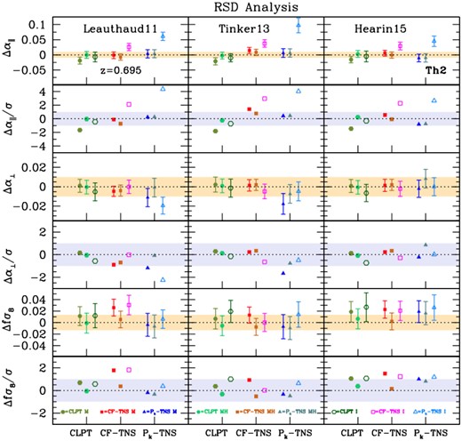
Full shape RSD analysis: main results on the AP parameters and the growth of structure. The three techniques adopted for the analysis of the final eBOSS LRG sample, two in configuration space (CLPT-GS and CF-TNS) and one in Fourier space (Pk-TNS), are confronted on a series of Outer Rim mocks having different HOD prescriptions. From left to right, the Leauthaud, Tinker, and Hearin models corresponding to ‘Th2’ are analysed, as they are closer to the characteristics of the eBOSS LRG sample. Individual fits on each of the 27 realizations per model are performed (open points), as well as fits on the mean of the mocks (filled points), allowing one to obtain accurate estimates of α∥, α⊥, and fσ8. Scatter plots in terms of σ-deviations are also shown. The shaded orange areas represent the |$1{{\ \rm per\ cent}}$| error levels on the α parameters and the |$3{{\ \rm per\ cent}}$| error on fσ8, while shaded grey areas highlight the 1σ error level. The corresponding numerical results are reported in Table B3. Errorbars follow the same conventions as in Fig. 10. See the main text for more details.
Overall, from the fit of the mean, biases observed for CLPT-GS and CF-TNS are mostly within 1.5σ away from the expected values for all the parameters across all models (and always less than 2σ away), and errors estimated from the different RSD models are mutually compatible. In general, CF-TNS seems to imply slightly larger errors than CLPT-GS. Comparing fits on the mean with the mean of individual fits, for α⊥ and fσ8 there is good agreement in values and errors. Also, for α∥, the fit of the mean is a more robust estimate of potential biases. The most significant differences are found for the best fits of α∥, but this comes with no surprise: it is in fact expected that fits on individual mocks are dominated by the low signal to noise, as the effective volume of a single OR mock is 1.10 Gpc3 – thus relatively small. Namely, given the low volume spanned by OR mocks, the fit to the mean and the mean of the fits differ, primarily because individual subcubes are dominated by noise and there are not enough subcubes for this effect to effectively cancel out. A good proof of this fact is provided by Fig. 10: when reconstruction is applied to the mocks (i.e. signal-to-noise increased), the differences between fits to the mean and mean of the fits shrink – as can be inferred by comparing the left-hand and right-hand panels of Fig. 10. Moreover, the ∼4σ discrepancy shown in Fig. 11 from individual fits to the Tinker model happens only for P(k) measurements, and affects primarily α∥ – the variable with the lowest signal (hence providing noisy spectra), as it depends only on the radial direction. In such case, very likely the fitting procedure tends to (incorrectly) identify the BAO signal in those noisier regions of the spectra; however, this does not happen for configuration space analyses, since the BAO signal is localized. In other terms, this is a clear example of inadequate BAO detections in individual fits. Finally, another source of discrepancy could be due to the rescaling for the ezmock covariance adopted in the analysis, that may not provide a full accurate description and causes a much larger variation on individual mocks.
In summary, from the results of fitting the mean, since we do not observe biases larger than 2σ, we conclude that different HODs do not have a significant impact in the fits even from an FS RSD analysis. This type of systematics is always below the statistical error of the LRG sample. It is also quite interesting to notice the remarkable consistency and (non-trivial) agreement between RSD FS techniques in configuration and Fourier space. In general, as demonstrated by Fig. 11, the HOD systematics derived from fits on the mean are within the |$\sim 1{{\ \rm per\ cent}}$| level, even smaller than the modelling systematics, and always below the statistical precision of the eBOSS LRG sample. The modelling systematics instead could reach the percentage level particularly in α∥ and fσ8, and could represent a dominant source of systematics. From a more extensive FS analysis, we thus conclude that while HOD systematics are subdominant to the global systematic error budget, the modelling systematics should be taken into account – although both are below the statistical precision of the eBOSS LRG sample. Moreover, from the FS study, we conclude that the different methodologies adopted for the analysis of the final eBOSS LRG sample are mutually consistent and robust, thus validating the clustering analysis pipelines.
6.4 Galaxy mock challenge: modelling systematics
The heterogeneous set of Outer Rim mocks previously adopted for assessing possible systematic effects in the galaxy–halo connection and imprecisions related to the galaxy clustering modelling (i.e. impact of HODs on BAO and RSD methods, and RSD modelling systematics) is suboptimal in accuracy at the sub-per cent level, although this type of accuracy is well-below the statistical sensitivity of the eBOSS LRG sample. This is mainly because of the relatively small effective volume spanned by each individual independent mock, due to the limitations posed by having only a single Outer Rim halo catalogue at z = 0.695 combined with the constraints intrinsic to the LRG modelling (see Section 3). For this reason, only 27 mocks were used in the previous analyses, as fully independent realizations (i.e. not sharing the same DM field) are required to properly assess cosmic variance. In terms of errorbars, the resolution limit of the OR mocks is in fact around the |$\sim\!1\!-\!2{{\ \rm per\ cent}}$| level. In order to evaluate the performance of the BAO and RSD modelling at a sub-per cent level, a more suitable choice is to abandon a single simulation – although of exquisite mass-resolution such as the Outer Rim – and opt instead for multiple realizations of the same box (i.e. identical initial conditions in all but the random seeds) at a lower mass-resolution and with a larger effective volume.8 This is the logic beyond the nseries, a small homogeneous set of 84 pseudo-independent mocks constructed from seven independent periodic boxes of |$2.6h^{-1}\, {\rm Gpc}$| side, projected through 12 different orientations and cuts per box; the mass resolution of these periodic boxes is much lower than that of the Outer Rim run, but it is still sufficient for resolving LRG-type haloes (|$1.5 \times 10^{11} \, h^{-1}\, \mathrm{M}_{\odot }$|, with 20483 particles per box). The global effective volume spanned is 84 × 3.67 [Gpc]3. The nseries are characterized by the same underlying galaxy bias model built upon the same cosmology, but each mock is a quasi-independent realization – thus not sharing exactly the same LSS – and including observational artefacts closer to the eBOSS DR16 sample, with similar angular and radial selection function of the observed sample. The HOD used is targeted to BOSS CMASS galaxies, at an effective redshift of |$\bar{z}=0.56$|. Although this set was originally devised for BOSS galaxies, it is still useful for evaluating modelling systematics at the sub-percentage level also for eBOSS tracers. This is why the nseries is extensively used in Bautista et al. (2020) and in Gil-Marín et al. (2020) for addressing the modelling systematics related to each complementary analysis in configuration and Fourier space, respectively. Here, we show only an interesting combined example, confronting the fitting methodologies in configuration and Fourier space and the performance of the RSD models previously introduced in Section 5.
Fig. 12 provides a summary result obtained by running the various BAO and RSD FS analysis pipelines on the average of 84 nseries mocks. Specifically, the left-hand panels display the AP parameters derived from a BAO-only fit in configuration and Fourier space, respectively. Filled symbols are used for pre-reconstructed catalogues, while open symbols refer to post-reconstructed catalogues. The left-hand panels show analogous quantities, as well as the growth of structure in terms of fσ8, derived from RSD FS fits. In this case the analysis is performed only over pre-reconstructed catalogues, and carried out in the nseries cosmology (see Section 4.2). Results from the three different RSD models – two in configuration space (CLPT-GS and CF-TNS) and one in Fourier space (Pk-TNS), all set for optimal performance as explained before, including the hexadecapole – are displayed with filled symbols. The corresponding numerical values are reported in Table B4. The grey areas in the figure highlight the |$0.5{{\ \rm per\ cent}}$| error level for the AP parameters, and the |$1.0{{\ \rm per\ cent}}$| error level for fσ8. As clearly seen, all the different methods are mutually consistent, showing a remarkable accuracy in recovering the expected cosmological parameters (α∥, α⊥, fσ8) at an exquisite level of precision, within at worst |$0.9{{\ \rm per\ cent}}$| of their expected values for the α’s and within |$1.5{{\ \rm per\ cent}}$| for fσ8 – as a conservative estimate. These results can be compared with analogous measurements performed on the Outer Rim mocks displayed in Figs 10 and 11. Although here at a sub-percentage level precision, results from the two different sets of mocks are consistent: we observe a similar trend at a fixed HOD recipe, indicating an impressive level of consistency between techniques in configuration and Fourier space. Clearly, the modelling systematics is addressed here with higher accuracy, showing deviations at the sub-per cent level for the AP parameters and fσ8. While this type of systematics may be a dominant source of error in the global systematic budget (despite sub-per cent deviations), the LRG sample is primarily dominated by the statistical error of the data.
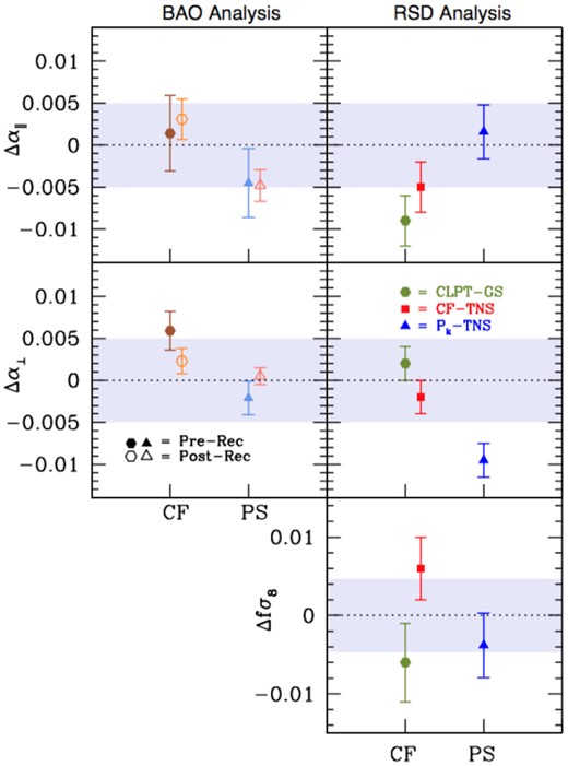
Comparing modelling systematics in BAO and RSD methods, estimated from 84 nseries mocks. Left-hand panels show the AP parameters derived from BAO-only fits in configuration and Fourier space, respectively. Right-hand panels refer to RSD full shape analyses. The filled symbols are used for pre-reconstructed catalogues, while open symbols refer to post-reconstructed catalogues. The gray areas in the figure highlight the |$0.5{{\ \rm per\ cent}}$| error level on α∥ and α⊥, and the |$1.0{{\ \rm per\ cent}}$| error on fσ8. These numerical results are reported in Table B4. All the different methods adopted for the clustering analysis of the eBOSS LRG sample are mutually consistent, showing a remarkable accuracy in recovering the expected cosmological parameters at an exquisite level of precision.
7 SYSTEMATIC ERROR BUDGET
Finally, we address here the LRG global error budget with a major focus on theoretical systematics, and also summarize the previous mock challenge results in term of biases in the estimation of α∥, α⊥, and fσ8.
7.1 Global error budget
Table 6 summarizes the global error budget for the eBOSS DR16 LRG sample. Here, the modelling systematics is inferred from the nseries (see Table B4) and indicated as |$\sigma _{\rm syst}^{\rm model, \rm {\small NS}}$|: we explain later on the reason behind this choice, and why the Outer Rim contribution is not included here. The comprehensive systematic error budget intrinsic to each RSD method (σsyst) is simply obtained by summing in quadrature the modelling and additional systematics, and the total error budget σtot is also derived in quadrature from the contributions of σsyst and σstat. In the table, we provide some useful ratios as well, that allow one to directly compare the contribution of systematics or statistics to the total error estimate. While the BAO-only pipeline is essentially unbiased, from the RSD FS analyses we conclude that systematic errors account for a significant fraction of the total error budget, contributing up to |$50{{\ \rm per\ cent}}$| (or more) to the uncertainties associated with the AP parameters and the growth of structures (see the various ratios). The impact in the determination of α∥ and α⊥ is at the |$\sim 1.0{{\ \rm per\ cent}}$| level, and it can reach even |$\sim\!1.5\!-\!2.0{{\ \rm per\ cent}}$| for fσ8. From configuration space analyses, the most relevant contribution to systematics is caused by observational artefacts. In Fourier space, the most dominant systematic is arising from the assumption of a reference cosmology, that can bias in particular the estimation of fσ8 up to |$2.0{{\ \rm per\ cent}}$|. All of the other effects, including modelling systematics, are within the |$1.0{{\ \rm per\ cent}}$| range or below. Eventually, systematic errors are added only to the diagonal of the covariance of each measurement, assuming that all the contributions to systematics are independent.
Global error budget for the final eBOSS DR16 LRG sample, as derived from configuration and Fourier space analyses.
| RSD-FS analysis | Global Syst. | |||
|---|---|---|---|---|
| Error type | Model | |$\sigma _{\alpha _\parallel }$| | |$\sigma _{\alpha _\perp }$| | |$\sigma _{\rm f \sigma _8}$| |
| RSD modelling | CLPT-GS | 0.0090 | 0.0040 | 0.0100 |
| |$[\sigma _{\rm syst}^{\rm model, \rm {\small NS}}]$| | CF-TNS | 0.0060 | 0.0040 | 0.0080 |
| Pk-TNS | 0.0064 | 0.0095 | 0.0082 | |
| RSD additional | CLPT-GS | 0.0156 | 0.0127 | 0.0220 |
| |$[\sigma _{\rm syst}^{\rm other}]$| | CF-TNS | 0.0153 | 0.0112 | 0.0216 |
| Pk-TNS | 0.0117 | 0.0068 | 0.0155 | |
| RSD systematics | CLPT-GS | 0.0180 | 0.0133 | 0.0242 |
| [σsyst] | CF-TNS | 0.0164 | 0.0119 | 0.0230 |
| Pk-TNS | 0.0133 | 0.0117 | 0.0175 | |
| RSD statistical | CLPT-GS | 0.0280 | 0.0200 | 0.0450 |
| [σstat] | CF-TNS | 0.0310 | 0.0180 | 0.0400 |
| Pk-TNS | 0.0360 | 0.0270 | 0.0420 | |
| RSD total | CLPT-GS | 0.0333 | 0.0240 | 0.0511 |
| [σtot] | CF-TNS | 0.0351 | 0.0216 | 0.0462 |
| Pk-TNS | 0.0384 | 0.0294 | 0.0455 | |
| CLPT-GS | 0.3214 | 0.2000 | 0.2222 | |
| |$\sigma _{\rm syst}^{\rm model, \rm {\small NS}}$|/σstat | CF-TNS | 0.1935 | 0.2222 | 0.2000 |
| Pk-TNS | 0.1778 | 0.3518 | 0.1952 | |
| CLPT-GS | 0.5571 | 0.6350 | 0.4889 | |
| |$\sigma _{\rm syst}^{\rm other}$|/σstat | CF-TNS | 0.4935 | 0.6222 | 0.5400 |
| Pk-TNS | 0.3250 | 0.2518 | 0.3690 | |
| CLPT-GS | 0.6432 | 0.6658 | 0.5370 | |
| σsyst/σstat | CF-TNS | 0.5301 | 0.6607 | 0.5758 |
| Pk-TNS | 0.3704 | 0.4327 | 0.4175 | |
| CLPT-GS | 0.2703 | 0.1665 | 0.1958 | |
| |$\sigma _{\rm syst}^{\rm model, \rm {\small NS}}$|/σtot | CF-TNS | 0.1710 | 0.1854 | 0.1733 |
| Pk-TNS | 0.1667 | 0.3229 | 0.1802 | |
| CLPT-GS | 0.4686 | 0.5286 | 0.4307 | |
| |$\sigma _{\rm syst}^{\rm other}$|/σtot | CF-TNS | 0.4361 | 0.5191 | 0.4679 |
| Pk-TNS | 0.3048 | 0.2311 | 0.3406 | |
| CLPT-GS | 0.5410 | 0.5542 | 0.4731 | |
| σsyst/σtot | CF-TNS | 0.4684 | 0.5513 | 0.4990 |
| Pk-TNS | 0.3474 | 0.3971 | 0.3853 | |
| CLPT-GS | 0.8410 | 0.8324 | 0.8810 | |
| σstat/σtot | CF-TNS | 0.8835 | 0.8343 | 0.8666 |
| Pk-TNS | 0.9378 | 0.9178 | 0.9228 |
7.2 Impact of modelling systematics
The modelling systematics estimated from ‘Th2’ Outer Rim mocks analysed in Section 6 are detailed in Table 7, where we list all the contributions inferred from the individual HODs of Leauthaud (LH), Tinker (TK), and Hearin (HE), respectively, as well as the combined theoretical systematics derived by simply averaging those contributions (|$\sigma _{\rm syst}^{\rm model, OR}$|). We also report some useful ratios, for the ease of comparison. Not surprisingly, the modelling systematics obtained from Outer Rim mocks are much larger than those derived from the nseries. The reason is related to the difference in effective volume, combined with the limited number of fully independent realizations available (27 synthetic catalogues per flavour). In fact, the global effective volume of ‘Th2’ Outer Rim mocks is 29.7 Gpc3, about 11 times bigger than the combined CMASS plus eBOSS LRG sample, but ∼10.27 times smaller than the global effective volume spanned by the nseries – which is 308.28 Gpc3, and thus 113 times larger than the combined DR16 LRG sample. In this respect, the statistical threshold of the nseries is at the |$0.1\!-\!0.5{{\ \rm per\ cent}}$| level, while the resolution of Outer Rim mocks is around |$1.0\!-\!1.5{{\ \rm per\ cent}}$|. As evident from Table 7, the modelling systematics inferred from Outer Rim mocks is closer to the statistical error of the LRG sample (see the various ratios |$\sigma _{\rm syst, LH}^{\rm model, OR}/\sigma _{\rm stat}$|, |$\sigma _{\rm syst, TK}^{\rm model, OR}/\sigma _{\rm stat}$|, |$\sigma _{\rm syst, HE}^{\rm model, OR}/\sigma _{\rm stat}$|), and a factor ∼2–5 times bigger than uncertainties derived from the nseries. The size of the errorbars simply scales with the global effective volume and the number of available realizations, as clearly highlighted by the various ratios |$\sigma _{\rm syst, LH}^{\rm model,OR}/\sigma _{\rm syst}^{\rm model,NS}$|, |$\sigma _{\rm syst, TK}^{\rm model,OR}/\sigma _{\rm syst}^{\rm model,NS}$|, and |$\sigma _{\rm syst, HE}^{\rm model,OR}/\sigma _{\rm syst}^{\rm model,NS}$|. This is the main reason why we omit to include these theoretical systematics in the previous global error budget, as the larger errorbars are primarily due to limited volume and statistics. Note, however, that the Outer Rim mocks are fully independent, and not pseudo-independent realizations, hence the errorbars are completely uncorrelated. After all, although closer to the statistical limit of the sample, the Outer Rim mocks allowed us to test and validate the robustness of the LRG analysis pipelines, the sensitivity to a number of HOD prescriptions, and to confirm the remarkable consistency across different methods in configuration and Fourier space.
| RSD-FS analysis | Model. Syst. | |||
|---|---|---|---|---|
| Systematic type | Model | |$\sigma _{\alpha _\parallel }$| | |$\sigma _{\alpha _\perp }$| | |$\sigma _{\rm f \sigma _8}$| |
| RSD modelling | CLPT-GS | 0.0228 | 0.0134 | 0.0330 |
| |$[\sigma _{\rm syst, LH}^{\rm model, \rm {\small OR}}]$| | CF-TNS | 0.0220 | 0.0104 | 0.0292 |
| Pk-TNS | 0.0276 | 0.0188 | 0.0400 | |
| RSD modelling | CLPT-GS | 0.0234 | 0.0154 | 0.0356 |
| |$[\sigma _{\rm syst, TK}^{\rm model, \rm {\small OR}}]$| | CF-TNS | 0.0204 | 0.0118 | 0.0280 |
| Pk-TNS | 0.0288 | 0.0214 | 0.0420 | |
| RSD modelling | CLPT-GS | 0.0218 | 0.0134 | 0.0356 |
| |$[\sigma _{\rm syst, HE}^{\rm model, \rm {\small OR}}]$| | CF-TNS | 0.0196 | 0.0124 | 0.0304 |
| Pk-TNS | 0.0258 | 0.0178 | 0.0380 | |
| RSD modelling | CLPT-GS | 0.0227 | 0.0141 | 0.0347 |
| |$[\sigma _{\rm syst}^{\rm model, \rm {\small OR}}]$| | CF-TNS | 0.0207 | 0.0115 | 0.0292 |
| Pk-TNS | 0.0274 | 0.0193 | 0.0400 | |
| CLPT-GS | 0.8143 | 0.6700 | 0.7334 | |
| |$\sigma _{\rm syst, LH}^{\rm model, \rm {\small OR}}$|/σstat | CF-TNS | 0.7097 | 0.5778 | 0.7300 |
| Pk-TNS | 0.7667 | 0.6963 | 0.9524 | |
| CLPT-GS | 0.8357 | 0.7700 | 0.7911 | |
| |$\sigma _{\rm syst, TK}^{\rm model, \rm {\small OR}}$|/σstat | CF-TNS | 0.6581 | 0.6556 | 0.7000 |
| Pk-TNS | 0.8000 | 0.7926 | 1.0000 | |
| CLPT-GS | 0.7786 | 0.6700 | 0.7911 | |
| |$\sigma _{\rm syst, HE}^{\rm model, \rm {\small OR}}$|/σstat | CF-TNS | 0.6323 | 0.6889 | 0.7600 |
| Pk-TNS | 0.7167 | 0.6593 | 0.9048 | |
| CLPT-GS | 0.8095 | 0.7033 | 0.7718 | |
| |$\sigma _{\rm syst}^{\rm model, \rm {\small OR}}$|/σstat | CF-TNS | 0.6667 | 0.6407 | 0.7300 |
| Pk-TNS | 0.7611 | 0.7160 | 0.9524 | |
| CLPT-GS | 2.5334 | 3.3500 | 3.3000 | |
| |$\sigma _{\rm syst, LH}^{\rm model, \rm {\small OR}}$|/|$\sigma _{\rm syst}^{\rm model, \rm {\small NS}}$| | CF-TNS | 3.6667 | 2.6000 | 3.6500 |
| Pk-TNS | 4.3125 | 1.9789 | 4.8781 | |
| CLPT-GS | 2.6000 | 3.8000 | 3.5600 | |
| |$\sigma _{\rm syst, TK}^{\rm model, \rm {\small OR}}$|/|$\sigma _{\rm syst}^{\rm model, \rm {\small NS}}$| | CF-TNS | 3.4000 | 2.9500 | 3.5000 |
| Pk-TNS | 4.5000 | 2.2526 | 5.1219 | |
| CLPT-GS | 2.4222 | 3.3500 | 3.5600 | |
| |$\sigma _{\rm syst, HE}^{\rm model, \rm {\small OR}}$|/|$\sigma _{\rm syst}^{\rm model, \rm {\small NS}}$| | CF-TNS | 3.2667 | 3.1000 | 3.8000 |
| Pk-TNS | 4.0312 | 1.8737 | 4.6341 | |
| CLPT-GS | 2.5185 | 3.5167 | 3.4733 | |
| |$\sigma _{\rm syst}^{\rm model, \rm {\small OR}}$|/|$\sigma _{\rm syst}^{\rm model, \rm {\small NS}}$| | CF-TNS | 3.4445 | 2.8834 | 3.6500 |
| Pk-TNS | 4.2812 | 2.0351 | 4.8780 |
8 CONCLUSIONS AND OUTLOOK
In support of the final analysis of the eBOSS DR16 galaxy sample, we have carried out an extensive N-body data challenge with the aim of testing and validating the robustness of the LRG clustering pipelines of Bautista et al. (2020) in configuration space, and of Gil-Marín et al. (2020) in Fourier space. We have also quantified the theoretical systematics related to BAO and RSD fitting methodologies, and the bias intrinsic to the modelling of the galaxy–halo connection.
To this end, we have constructed new heterogeneous galaxy mocks from the Outer Rim simulation spanning different redshift intervals, using a variety of HOD schemes of increasing complexity and characterized by analogous clustering properties. The theoretical foundation for modelling the galaxy–halo connection is laid out in Section 3, and the mock-making procedure is explained in detail in Section 4. Moving from the most conventional HOD approach, we have considered more sophisticated scenarios able to distinguish between quiescent or star-forming galaxies, and with the inclusion of assembly bias that generalize further the standard HOD framework. Our Outer Rim-based mocks cover a range of number densities and effective volumes, and are well-suited for a variety of studies. In this work, we have mainly focused on a subset at z = 0.695, with characteristics closer to the eBOSS LRG sample (i.e. ‘Th2’ flavour with the Leauthaud, Tinker, and Hearin prescriptions). We have also briefly exploited a small homogeneous synthetic set (the nseries), which has been previously used in the SDSS DR12 galaxy clustering analysis and is more suitable to assess theoretical systematics at the sub-per cent level, thanks to a larger effective volume.
In our challenge, detailed in Section 6, we have tested the performance of BAO and RSD fitting techniques against different galaxy population schemes and bias models having analogous clustering properties, with the main objective of validation and calibration of such methods and the quantification of theoretical systematics. The mock products have allowed us to confront on a common ground and assess the performance of the BAO fitting methodologies for the LRG sample, and of three complementary RSD models in configuration and Fourier space – denoted as CLPT-GS, CF-TNS, and Pk-TNS, respectively. Overall, we have found a remarkable agreement at the sub-per cent level between different techniques in configuration and Fourier space (see in particular Figs 10, 11, and 12), along with an impressive level of consistency among BAO fitting and reconstruction procedures and from all the RSD models used in FS analyses. All of the methods performed equally well, with comparable errors on the AP parameters and the growth of structure. Moreover, reconstruction significantly improved the constraints on both α∥ and α⊥. We have thus validated the robustness of the LRG clustering analysis pipelines.
Including in our analysis the complexity of more sophisticated HODs schemes that go beyond the traditional mass-only ansatz, such as models with central and satellite velocity bias (Tinker 2007; Guo et al. 2015), generalizations of the standard five parameter HOD model with various halo-scale physics (Yuan et al. 2018; Duan & Eisenstein 2019; Xu et al. 2020; Xu & Zheng 2020), and forward-modelling approaches using satellite kinematics (Lange et al. 2019a, b; van den Bosch, Lange & Zentner 2019) is left to future studies. However, as pointed out by Duan & Eisenstein (2019), only a rather unrealistic extreme level of velocity bias of the central galaxies would produce a shift of 0.7 per cent in the LOS acoustic scale, and basically other bias models including satellite velocity bias are consistent with zero shift at the 0.2 per cent level after reconstruction. Since current surveys such as eBOSS measure the acoustic scale to |$\sim 1{{\ \rm per\ cent}}$| precision, they are insensitive to the galaxy bias effect – and we expect that similar conclusions will hold for the related AP parameters.
Regarding systematics and the global error budget (Section 7), we have found that the impact of different HOD prescriptions is always sub-dominant to the total systematics, and that modelling systematics in the estimation of α∥ and fσ8, although at worst around |$\sim 1.5{{\ \rm per\ cent}}$|, may be a dominant source of error in the comprehensive quantification of systematics. In particular, from the analysis in configuration space of pre-reconstructed mocks (considering only fits to the mean), biases in the recovered α values reach up to |$0.5{{\ \rm per\ cent}}$| in α⊥ and |$1.0{{\ \rm per\ cent}}$| in α∥. After reconstruction, there is a reduction of the biases to less than |$0.2{{\ \rm per\ cent}}$|, hence the BAO analysis is unbiased. For RSD analyses in configuration space, the most significant contribution to systematic errors arises from observational effects. From the Fourier space methodology, for the post-reconstruction BAO analysis we detected a |$0.5{{\ \rm per\ cent}}$| systematic shift induced by modelling systematic on α∥, and none for α⊥, with a resolution limit of |$0.2{{\ \rm per\ cent}}$| for the nseries mocks. The systematic shift is of order |$1.5{{\ \rm per\ cent}}$| for the FS analysis from Outer Rim mocks instead. Moreover, we did not detect any significant relative shift on the cosmological parameters when either the HOD model or the flavour is varied. Such results put constrains in the upper limit of systematic errors in the modelling, as a result of different HODs, with upper limits of order |$0.5\!-\!1.1{{\ \rm per\ cent}}$| systematic shifts. In any case, both HOD and modelling systematics are below the statistical error of the eBOSS LRG data. The expected statistical errors in the eBOSS LRG data sample are in fact of the order of |$\sim 1.9{{\ \rm per\ cent}}$| for α⊥, and |$\sim 2.6{{\ \rm per\ cent}}$| for α∥. Eventually, these systematic corrections in the AP parameters and the growth of structure are combined with additional sources of systematics (Table 6), and such errors are accounted for in the final consensus results (eBOSS Collaboration 2020) from the analysis of the LRG DR16 galaxy sample. Finally, our analysis provides a global and complementary perspective of the systematic studies carried out in Bautista et al. (2020) in configuration space, and in Gil-Marín et al. (2020) in Fourier space: their overall agreement at such level of precision is remarkable.
Quantifying the modelling systematics in BAO clustering estimators and in RSD methods for all the eBOSS tracers, as well as characterizing the robustness of the analysis pipelines, are essential tasks in order to obtain unbiased cosmological parameters, accurate fσ8 constraints, and reliable consensus likelihoods. In this respect, besides being relevant for the final eBOSS DR16 ‘consensus cosmology’ – as the systematic error budget is informed by testing the results of analyses against these high-resolution mocks – our study represents also a testbed for future large-volume surveys. In particular, similar mock-making techniques and systematic corrections can be readily extended to model for instance the DESI galaxy sample, and we expect that more extensive mock challenges along these lines will be necessary and progressively relevant in the next few years. In fact, mock challenges designed to validate data analysis pipelines and assess the impact of systematics in massive data sets are becoming increasingly important for large-volume surveys – see for example the recent works by MacCrann et al. (2018) for the Dark Energy Survey (DES; The Dark Energy Survey Collaboration 2005), and by Sánchez et al. (2020) for LSST (Ivezić et al. 2019). In this view, while the sub-per cent level theoretical systematic corrections quantified in this study may not be relevant for the current state of the art (as they are always inferior to the statistical precision of the data), soon they will become relevant for DESI and LSST, that are expected to achieve sub-per cent statistical precision on the galaxy sample; for such surveys, it will be crucial to control the systematics at an extremely low level. To this end, our flexible and highly modular pipeline for building complex HODs offers several directions of extension, as well as applications that go beyond the modelling of LRGs – toward more elaborated galaxy–halo connection physics, particularly in relation to ELGs.
ACKNOWLEDGEMENTS
GR, PDC, and JM acknowledge support from the National Research Foundation of Korea (NRF) through Grants No. 2017R1E1A1A01077508 and No. 2020R1A2C1005655 funded by the Korean Ministry of Education, Science and Technology (MoEST), and from the faculty research fund of Sejong University. GR was on sabbatical leave in 2020, when this research was completed. Some numerical work performed in this paper was carried out using the Korea Institute of Science and Technology Information (KISTI) supercomputing infrastructure under allocations KSC-2018-G3-0008 and KSC-2018-T1-0061, and with computing resources at Sejong University (Xeon Silver 4114 master node and Xeon Gold 6126 computing node architecture).
HGM acknowledges support from la Caixa Foundation (ID 100010434) which code LCF/BQ/PI18/11630024.
RP, SdlT, and SE acknowledge support from the eBOSS ANR grant (under contract ANR-16-CE31-0021) and the OCEVU LABEX (Grant No. ANR-11-LABX-0060) of the French National Research Agency.
Funding for the Sloan Digital Sky Survey IV has been provided by the Alfred P. Sloan Foundation, the U.S. Department of Energy Office of Science, and the Participating Institutions. SDSS-IV acknowledges support and resources from the Center for High-Performance Computing at the University of Utah. The SDSS web site is www.sdss.org.
SDSS-IV is managed by the Astrophysical Research Consortium for the Participating Institutions of the SDSS Collaboration including the Brazilian Participation Group, the Carnegie Institution for Science, Carnegie Mellon University, the Chilean Participation Group, the French Participation Group, Harvard-Smithsonian Center for Astrophysics, Instituto de Astrofísica de Canarias, The Johns Hopkins University, Kavli Institute for the Physics and Mathematics of the Universe (IPMU) / University of Tokyo, the Korean Participation Group, Lawrence Berkeley National Laboratory, Leibniz Institut für Astrophysik Potsdam (AIP), Max-Planck-Institut für Astronomie (MPIA Heidelberg), Max-Planck-Institut für Astrophysik (MPA Garching), Max-Planck-Institut für Extraterrestrische Physik (MPE), National Astronomical Observatories of China, New Mexico State University, New York University, University of Notre Dame, Observatário Nacional / MCTI, The Ohio State University, Pennsylvania State University, Shanghai Astronomical Observatory, United Kingdom Participation Group, Universidad Nacional Autónoma de México, University of Arizona, University of Colorado Boulder, University of Oxford, University of Portsmouth, University of Utah, University of Virginia, University of Washington, University of Wisconsin, Vanderbilt University, and Yale University.
In addition, this research relied on resources provided to the eBOSS Collaboration by the National Energy Research Scientific Computing Center (NERSC). NERSC is a U.S. Department of Energy Office of Science User Facility operated under Contract No. DE-AC02-05CH11231.
DATA AVAILABILITY
All of the SDSS mock products developed in this study, listed in Table A1, are stored at the National Energy Research Scientific Computing Center (NERSC) and are available upon request. The Outer Rim halo catalogues used to produce the Outer Rim-based mocks are publicly available at https://cosmology.alcf.anl.gov.
Footnotes
A description of eBOSS and a link to its associated publications can be found at this URL: https://www.sdss.org/surveys/eboss/.
Throughout the paper, we implicitly assume base 10 for all the logarithmic notations indicated with log, namely log ≡ log10, and drop the understood subscript for clarity of notation.
As pointed out by Zheng et al. (2007), Mmin can also be interpreted as the mass of such haloes for which half of them host galaxies above the given luminosity threshold, i.e. 〈Ncen(Mmin)〉 = 0.5.
The Outer Rim halo catalogues used here are publicly available at https://cosmology.alcf.anl.gov
We have also devised an additional set which includes a variety of customizations, beyond the scope of the current analysis, exploring extreme variations in HOD parameters for all of the models, quenching, assembly bias, and modulations with the central distribution.
Another alternative would be to pursue instead a subhalo-type modelling approach, rather than the more traditional HOD framework, but we do not have access to full merger trees from the Outer Rim simulation.
REFERENCES
APPENDIX A: MOCK PRODUCTS
We have devised three sets of heterogeneous Outer Rim-based galaxy mocks (indicated as ‘Challenge Set 1’, ‘Challenge Set 2’, ‘Challenge Set 3’, respectively) for the galaxy mock challenge. These are cubic mocks, in the Outer Rim cosmology, obtained by populating Outer Rim halo catalogues with galaxies as explained in Section 4.1. Details regarding each set are provided next.
Specifically, ‘Challenge Set 1’ (HOD VARIATIONS) contains a total of 3240 mocks (1620 at z = 0.695, and 1620 at z = 0.865), grouped into four model categories according to the underlying HOD scheme (i.e. Zheng, Leauthaud, Tinker, Hearin); each model category consists of three ‘flavours’, denoted as ‘Standard’ (Std), ‘Threshold 1’ (Th1), and ‘Threshold 2’ (Th2). As explained in Sections 3 and 4.4, the meaning of ‘flavour’ is related to the key parameter ‘threshold’, which globally sets all the individual HOD parameters as best-fitting realizations from the corresponding literature dictionary of each HOD model (unless specific customizations are introduced). At a given redshift, we produced 135 mocks per model flavour, by populating the full |$3 \, h^{-1} \, {\rm Gpc}$| Outer Rim periodic halo catalogue box five times, and then cutting each full box into 27 subcubes of |$1h^{-1}\, {\rm Gpc}$| side and rescaling the various spatial positions accordingly. This means that effectively we have 27 fully independent (i.e. not sharing the same DM field) mocks per realization, and each of these 27 mocks will have five different replicas. According to the modelling explained in Section 3, central galaxies are always located at the centre of their parent haloes with identical velocities, while the satellite population is statistically different in all the realizations – assuming a NFW profile. We then add RSDs to each individual mock in two different ways: radially, or with the usual plane-parallel approximation. This is the primary set considered in our main analysis presented in Section 6.
‘Challenge Set 2’ (REDSHIFT EVOLUTION) is similar to the previous one, but now the redshift evolution is taken into account for one threshold flavour and three different HOD prescriptions. In detail, we consider seven redshift intervals, namely z = 0.402, 0.502, 0.618, 0.695, 0.779, 0.865, 1.006, and produced a set of 2835 mocks (135 × 7 × 3) with three HOD schemes (Leauthaud, Tinker, Hearin), for the ‘Th1’ flavour. Even in this case, we consider subcubes of |$1h^{-1}\, {\rm Gpc}$| side.
Finally, ‘Challenge Set 3’ (HOD VARIATIONS / LARGE BOX) is similar to the first one, but in this case we exploit the full Outer Rim box (|$3h^{-1}\, {\rm Gpc}$|) with periodic boundary conditions rather than subcubes, and produced 100 realizations per flavour for all the HODs and thresholds considered in the first set – for a total of 2400 mocks. If desirable, these large-box realizations can be casted into smaller pseudo-independent mocks by performing cuts along different directions of the boxes, and also via the inclusion of partial overlaps in order to maximize the effective volume.
Regardless of the specific set, each mock contains the following information: galaxy spatial positions (in |$h^{-1}\, {\rm Mpc}$|), galaxy velocities (in comoving km s−1), the galaxy type (central, satellite), the number of centrals that a halo hosts (either 0 or 1), the number of satellites per halo, the global ID of the halo a galaxy belongs to, the halo mass and virial radius, the central star formation designation for some models (active, quiescent), the number of active or quiescent satellites, and the percentile spit in concentration for models with assembly bias.
A summary of all the synthetic products available, categorized by HOD and redshift, is provided in Table A1. While only a subset of these mocks is used for testing the BAO templates and the RSD models adopted for the characterization of LRG clustering systematics, with this work we release the entire suite of products – that are suitable to several interesting applications.
List of Outer Rim synthetic products developed for the galaxy mock challenge.
| Set | HOD Style | HOD Flavour | Redshift | Box [|$h^{-1}\, {\rm Gpc}$|] | Total mocks |
|---|---|---|---|---|---|
| Zheng07 | Th1, Std, Th2 | 0.695, 0.865 | 1.0 | 810 | |
| Challenge Set 1 | Leauthaud11 | Th1, Std, Th2 | 0.695, 0.865 | 1.0 | 810 |
| Tinker13 | Th1, Std, Th2 | 0.695, 0.865 | 1.0 | 810 | |
| Hearin15 | Th1, Std, Th2 | 0.695, 0.865 | 1.0 | 810 | |
| 3240 | |||||
| Leauthaud11 | Th1 | 0.402, 0.502, 0.618, 0.695, 0.779, 0.865, 1.006 | 1.0 | 945 | |
| Challenge Set 2 | Tinker13 | Th1 | 0.402, 0.502, 0.618, 0.695, 0.779, 0.865, 1.006 | 1.0 | 945 |
| Hearin15 | Th1 | 0.402, 0.502, 0.618, 0.695, 0.779, 0.865, 1.006 | 1.0 | 945 | |
| 2835 | |||||
| Zheng07 | Th1, Std, Th2 | 0.695, 0.865 | 3.0 | 600 | |
| Challenge Set 3 | Leauthaud11 | Th1, Std, Th2 | 0.695, 0.865 | 3.0 | 600 |
| Tinker13 | Th1, Std, Th2 | 0.695, 0.865 | 3.0 | 600 | |
| Hearin15 | Th1, Std, Th2 | 0.695, 0.865 | 3.0 | 600 | |
| 2400 |
Table A2 reports the number densities of the challenge mocks, expressed in units of 10−4[h3Mpc−3], and ordered by HOD type and flavour. The ‘Th2’ models of Leauthaud, Tinker, and Hearin are those characterized by a number density closer to the eBOSS LRG sample (see e.g. fig. 1 in Gil-Marín et al. 2020 and fig. 1 in Bautista et al. 2020 for details), and are extensively used in Section 6 to test the LRG BAO and RSD analysis pipelines. The other threshold levels are more suitable for example for assessing the details of the satellite distributions and for studying the galaxy–halo connection, particularly in relation to ELGs; they are only marginally explored in this work, although of high interest, and left to future applications.
Number densities of the challenge mocks listed in Table A1, ordered per HOD type and flavour.
| Number density [|$10^{-4} \, (h^3\, {\rm Mpc}^{-3})$|] | |||
|---|---|---|---|
| HOD model | Th1 | Std | Th2 |
| Zheng07 | 67.05 | 34.26 | 5.64 |
| Leauthaud11 | 50.55 | 11.85 | 0.69 |
| Tinker13 | 26.37 | 8.12 | 0.79 |
| Hearin15 | 44.93 | 10.82 | 0.69 |
| Number density [|$10^{-4} \, (h^3\, {\rm Mpc}^{-3})$|] | |||
|---|---|---|---|
| HOD model | Th1 | Std | Th2 |
| Zheng07 | 67.05 | 34.26 | 5.64 |
| Leauthaud11 | 50.55 | 11.85 | 0.69 |
| Tinker13 | 26.37 | 8.12 | 0.79 |
| Hearin15 | 44.93 | 10.82 | 0.69 |
Fig. A1 shows examples of the 3D galaxy clustering quantified by the 2-point spatial correlation ξ(r), as a function of separation r. The various measurements are performed at z = 0.695 (top panels) and at z = 0.865 (bottom panels), for the mocks belonging to ‘Challenge Set 1’. From left to right, the ‘Th1’, ‘Std’, and ‘Th2’ flavours are displayed, respectively. The HOD models of Leauthaud (blue), Tinker (red), and Hearin (green) are displayed with different colours: they are characterized by approximately similar clustering properties, at a fixed threshold level. Each measurement represents an average over 135 mocks, according to the specific HOD style and flavour, and errorbars are 1σ variations. The effect of a decreasing number density (from left to right) is of an overall increase in the clustering and BAO peak amplitude, with a relatively small redshift dependence.
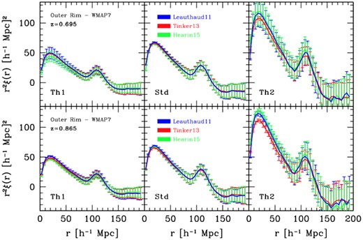
Clustering properties of the ‘Challenge Set 1’. Examples of 2-point spatial correlation functions computed at z = 0.695 (top panels) and at z = 0.865 (bottom panels), for the three threshold levels denoted as ‘Th1’, ‘Std’, and ‘Th2’ – in decreasing number density order, from left to right. The Leauthaud (blue), Tinker (red), and Hearin (green) HOD models are displayed with different colours. They are characterized by approximately similar clustering properties, at a fixed threshold level.
Finally, Fig. A2 displays an example of the 2-point spatial clustering of satellites, split by active/star-forming (blue) and quiescent (red) galaxies, at z = 0.865 for the ‘Std’ threshold level (see Table A2). The Tinker HOD formalism used in this work – primarily for LRG studies – could also potentially provide interesting applications to ELGs that go beyond the scope of this paper, and that highlight the flexibility of our mock-making procedure and mock products in exploring the physics of the galaxy–halo connection.
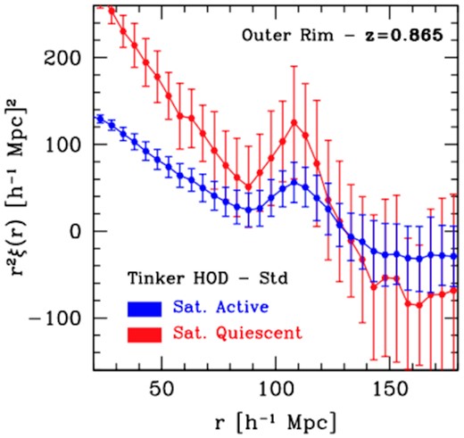
Spatial clustering of satellite galaxies at z = 0.865, split by active/star-forming (blue) and quiescent (red) – as described by the Tinker model for the ‘Std’ threshold level. This more complex HOD framework provides interesting insights on the galaxy–halo connection physics.
APPENDIX B: USEFUL TABLES
We provide here some useful tables with numerical results that appear in the various plots displayed in the manuscript, for the ease of direct comparisons, or that include additional information not reported in the main text.
Specifically, Table B1 contains results from the BAO and RSD analyses in Fourier space related to the Zheng model – see also our companion paper Gil-Marín et al. (2020) for additional extensive details.
Impact of the Zheng HOD model, presented in three different flavours (see Table 1), on pre-reconstructed BAO and FS fits on OR cubic boxes (1|$h^{-1}\, {\rm Gpc}$|; ‘Challenge Set 1’), from a Fourier space analysis. For simplicity, only the fit to the mean is provided – see Gil-Marín et al. (2020) for extensive details.
| Analysis type | HOD type | HOD flavour | |$\alpha _\parallel -\alpha _\parallel ^{\rm exp}$| | |$\alpha _\perp -\alpha _\perp ^{\rm exp}$| | |$f\sigma _8 - f\sigma _8^{\rm exp}$| |
|---|---|---|---|---|---|
| BAO Fourier space | Zheng | Th1 | 0.0270 ± 0.0110 | −0.0006 ± 0.0062 | – |
| [Pre-Rec] | Zheng | Std | 0.0240 ± 0.0100 | −0.0005 ± 0.0060 | – |
| Zheng | Th2 | 0.0310 ± 0.0130 | −0.0014 ± 0.0075 | – | |
| RSD Fourier space | Zheng | Th1 | 0.0107 ± 0.0069 | −0.0035 ± 0.0052 | −0.0085 ± 0.0073 |
| [Pre-Rec] | Zheng | Std | 0.0108 ± 0.0067 | −0.0025 ± 0.0051 | −0.0083 ± 0.0065 |
| Zheng | Th2 | 0.0138 ± 0.0095 | −0.0049 ± 0.0072 | 0.0080 ± 0.0130 |
Table B2 reports the results when fitting the mean correlation functions and power spectra (rows labelled ‘Mean’) of a set of 27 independent realizations of the OR-based mocks with different HOD prescriptions (‘Challenge Set 1’), as well as the mean of the fits of individual realizations (rows labelled ‘Individual’), in relation to the BAO analyses presented in Section 6.2.
Performance of the BAO templates on OR-based mocks, for the ‘Th2’ flavour and different HOD models. Mocks are analysed in their own Outer Rim cosmology, so the expected values for both α∥ and α⊥ are 1. For each set of mocks, the results from pre- and post-reconstruction catalogues are presented. We report both the results of fitting the mean of all the mocks, indicated with ‘Mean’, and the mean of individual fits on the mocks, indicated as ‘Individual’. For the fit to the mean, the error quoted is the 1σ of the error on this fit, where the covariances are scaled by the 27 Outer Rim realizations per HOD used to compute the mean. For the mean of individual best-fits, the error quoted is the rms divided by |$\sqrt{N_{\rm OR}}$|, where NOR = 27. The average of the best-fits is then performed over NOR. Consequently, the errors of ‘Mean’ and ‘Individual’ are comparable. Results of these fits are displayed in Fig. 10.
| BAO analysis type | HOD Type | HOD flavour | Analysis details | |$\alpha _\parallel -\alpha _\parallel ^{\rm exp}$| | |$\alpha _\perp -\alpha _\perp ^{\rm exp}$| | Ndet/Ntot |
|---|---|---|---|---|---|---|
| Configuration space | Leauthaud | Th2 | Mean | 0.0084 ± 0.0164 | −0.0010 ± 0.0080 | 1/1 |
| [Pre-Rec] | Leauthaud | Th2 | Individual | 0.0283 ± 0.0197 | −0.0072 ± 0.0123 | 27/27 |
| Tinker | Th2 | Mean | 0.0234 ± 0.0147 | −0.0078 ± 0.0073 | 1/1 | |
| Tinker | Th2 | Individual | 0.0166 ± 0.0172 | 0.0000 ± 0.0104 | 27/27 | |
| Hearin | Th2 | Mean | 0.0040 ± 0.0157 | 0.0074 ± 0.0083 | 1/1 | |
| Hearin | Th2 | Individual | 0.0035 ± 0.0185 | 0.0090 ± 0.0089 | 27/27 | |
| Configuration space | Leauthaud | Th2 | Mean | −0.0063 ± 0.0084 | 0.0045 ± 0.0056 | 1/1 |
| [Post-Rec] | Leauthaud | Th2 | Individual | −0.0050 ± 0.0108 | 0.0053 ± 0.0063 | 27/27 |
| Tinker | Th2 | Mean | −0.0024 ± 0.0090 | 0.0014 ± 0.0060 | 1/1 | |
| Tinker | Th2 | Individual | 0.0078 ± 0.0103 | −0.0017 ± 0.0065 | 27/27 | |
| Hearin | Th2 | Mean | 0.0115 ± 0.0094 | 0.0066 ± 0.0057 | 1/1 | |
| Hearin | Th2 | Individual | 0.0019 ± 0.0097 | 0.0087 ± 0.0054 | 27/27 | |
| Fourier space | Leauthaud | Th2 | Mean | −0.0114 ± 0.0178 | 0.0028 ± 0.0107 | 1/1 |
| [Pre-Rec] | Leauthaud | Th2 | Individual | 0.0000 ± 0.0180 | 0.0110 ± 0.0120 | 27/27 |
| Tinker | Th2 | Mean | 0.0023 ± 0.0177 | −0.0047 ± 0.0124 | 1/1 | |
| Tinker | Th2 | Individual | −0.0110 ± 0.0160 | 0.0230 ± 0.0110 | 27/27 | |
| Hearin | Th2 | Mean | −0.0221 ± 0.0143 | 0.0108 ± 0.0099 | 1/1 | |
| Hearin | Th2 | Individual | −0.0210 ± 0.0160 | 0.0160 ± 0.0110 | 27/27 | |
| Fourier space | Leauthaud | Th2 | Mean | −0.0062 ± 0.0104 | −0.0024 ± 0.0075 | 1/1 |
| [Post-Rec] | Leauthaud | Th2 | Individual | 0.0020 ± 0.0130 | −0.0093 ± 0.0074 | 27/27 |
| Tinker | Th2 | Mean | −0.0024 ± 0.0121 | −0.0025 ± 0.0088 | 1/1 | |
| Tinker | Th2 | Individual | 0.0038 ± 0.0097 | −0.0006 ± 0.0072 | 27/27 | |
| Hearin | Th2 | Mean | 0.0002 ± 0.0113 | 0.0122 ± 0.0075 | 1/1 | |
| Hearin | Th2 | Individual | 0.0090 ± 0.0150 | 0.0167 ± 0.0061 | 27/27 |
Table B3 reports the main results of the RSD FS analyses presented in Section 6.3, confronting the three different modelling techniques: two in configuration space (CLPT-GS and CF-TNS), and one in Fourier space (Pk-TNS). Individual fits on each of the 27 realizations per model are performed, as well as fits on the mean of the mocks.
Performance of the RSD FS methods evaluated on the OR-based mocks, for the ‘Th2’ flavour with different HOD models. Mocks are analysed in their own Outer Rim cosmology, so the expected values are 1 for the α parameters and |$f\sigma _8^{\rm exp} = 0.447$|. For each set of mocks, the results from pre-reconstructed catalogues are presented. We report both the results of fitting the mean of all the 27 realization per HOD, indicated with ‘Mean’, and the mean of individual fits on the mocks, indicated as ‘Individual’. For the fit to the mean, the error quoted is the 1σ of the error on the fit, where the covariances are scaled by the 27 realizations. For the mean of individual best-fits, the error quoted is the rms divided by the number of realizations. These results are visualized in Fig. 11.
| RSD analysis type | HOD type | HOD flavour | Analysis details | |$\alpha _\parallel -\alpha _\parallel ^{\rm exp}$| | |$\alpha _\perp -\alpha _\perp ^{\rm exp}$| | |$f\sigma _8 - f\sigma _8^{\rm exp}$| | Ndet/Ntot |
|---|---|---|---|---|---|---|---|
| Configuration space | Leauthaud | Th2 | Mean | −0.0189 ± 0.0114 | 0.0010 ± 0.0067 | 0.0113 ± 0.0165 | 1/1 |
| [Pre-Rec] | Leauthaud | Th2 | Individual | −0.0069 ± 0.0159 | −0.0052 ± 0.0092 | 0.0119 ± 0.0209 | 27/27 |
| CLPT-GS | Tinker | Th2 | Mean | −0.0211 ± 0.0117 | 0.0022 ± 0.0077 | 0.0066 ± 0.0178 | 1/1 |
| Tinker | Th2 | Individual | −0.0096 ± 0.0135 | −0.0014 ± 0.0093 | 0.0193 ± 0.0193 | 27/27 | |
| Hearin | Th2 | Mean | −0.0158 ± 0.0109 | 0.0008 ± 0.0067 | 0.0187 ± 0.0178 | 1/1 | |
| Hearin | Th2 | Individual | −0.0053 ± 0.0176 | −0.0065 ± 0.0089 | 0.0267 ± 0.0250 | 27/27 | |
| Configuration space | Leauthaud | Th2 | Mean | −0.0012 ± 0.0110 | −0.0046 ± 0.0052 | 0.0260 ± 0.0146 | 1/1 |
| [Pre-Rec] | Leauthaud | Th2 | Individual | 0.0259 ± 0.0122 | −0.0001 ± 0.0069 | 0.0305 ± 0.0168 | 27/27 |
| CF-TNS | Tinker | Th2 | Mean | 0.0144 ± 0.0102 | 0.0014 ± 0.0059 | 0.0130 ± 0.0140 | 1/1 |
| Tinker | Th2 | Individual | 0.0375 ± 0.0126 | −0.0049 ± 0.0076 | 0.0002 ± 0.0157 | 27/27 | |
| Hearin | Th2 | Mean | 0.0056 ± 0.0098 | 0.0014 ± 0.0062 | 0.0227 ± 0.0152 | 1/1 | |
| Hearin | Th2 | Individual | 0.0291 ± 0.0127 | −0.0022 ± 0.0077 | 0.0205 ± 0.0168 | 27/27 | |
| Fourier space | Leauthaud | Th2 | Mean | 0.0034 ± 0.0138 | −0.0111 ± 0.0094 | −0.0040 ± 0.0200 | 1/1 |
| [Pre-Rec] | Leauthaud | Th2 | Individual | 0.0610 ± 0.0140 | −0.0195 ± 0.0087 | 0.0060 ± 0.0160 | 27/27 |
| Pk-TNS | Tinker | Th2 | Mean | 0.0060 ± 0.0144 | −0.0177 ± 0.0107 | −0.0070 ± 0.0210 | 1/1 |
| Tinker | Th2 | Individual | 0.0970 ± 0.0240 | −0.0047 ± 0.0097 | 0.0140 ± 0.0220 | 27/27 | |
| Hearin | Th2 | Mean | −0.0104 ± 0.0129 | −0.0020 ± 0.0089 | 0.0190 ± 0.0190 | 1/1 | |
| Hearin | Th2 | Individual | 0.0450 ± 0.0170 | 0.0001 ± 0.0093 | 0.0260 ± 0.0220 | 27/27 |
Finally, Table B4 provides the numerical results obtained by running the various BAO and RSD FS analysis pipelines on the average of 84 nseries mocks, as detailed in Section 6.4. The analysis is performed only over pre-reconstructed catalogues, and carried out in the nseries cosmology (Section 4.2).
Modelling systematics related to BAO and RSD methodologies, addressed with the nseries. These numerical results are shown in Fig. 12.
| Analysis Type | Analysis space | Analysis method | Fitting model | |$\alpha _\parallel -\alpha _\parallel ^{\rm exp}$| | |$\alpha _\perp -\alpha _\perp ^{\rm exp}$| | |$f\sigma _8 - f\sigma _8^{\rm exp}$| |
|---|---|---|---|---|---|---|
| BAO [Pre-Rec] | Configuration space | CF – BAO Peak | BAO Template | 0.0014 ± 0.0045 | 0.0059 ± 0.0023 | – |
| BAO [Pre-Rec] | Fourier space | PS – BAO Peaks | BAO Template | −0.0045 ± 0.0041 | −0.0021 ± 0.0020 | – |
| BAO [Post-Rec] | Configuration space | CF – BAO Peak | BAO Template | 0.0031 ± 0.0024 | 0.0023 ± 0.0015 | – |
| BAO [Post-Rec] | Fourier space | PS – BAO Peaks | BAO Template | −0.0048 ± 0.0019 | 0.0005 ± 0.0010 | – |
| RSD [Pre-Rec] | Configuration space | CF – Full Shape | CLPT-GS | −0.0090 ± 0.0030 | 0.0020 ± 0.0020 | −0.0060 ± 0.0050 |
| RSD [Pre-Rec] | Configuration space | CF – Full Shape | CF-TNS | −0.0050 ± 0.0030 | −0.0020 ± 0.0020 | 0.0060 ± 0.0040 |
| RSD [Pre-Rec] | Fourier space | PS – Full Shape | Pk-TNS | 0.0016 ± 0.0032 | −0.0095 ± 0.0020 | −0.0038 ± 0.0041 |
