A multishock model for the density variance of anisotropic, highly magnetized, supersonic turbulence

Beattie, James R; Mocz, Philip; Federrath, Christoph; Klessen, Ralf S

doi:10.1093/mnras/stab1037

ABSTRACT

Shocks form the basis of our understanding for the density and velocity statistics of supersonic turbulent flows, such as those found in the cool interstellar medium (ISM). The variance of the density field, |$\sigma ^2_{\rho /\rho _0}$|⁠, is of particular interest for molecular clouds (MCs), the birthplaces of stars in the Universe. The density variance may be used to infer underlying physical processes in an MC, and parametrizes the star formation (SF) rate of a cloud. However, models for |$\sigma ^2_{\rho /\rho _0}$| all share a common feature – the variance is assumed to be isotropic. This assumption does not hold when a trans-/sub-Alfvénic mean magnetic field, |${B}_0$|⁠, is present in the cloud, which observations suggest is relevant for some MCs. We develop an anisotropic model for |$\sigma _{\rho /\rho _0}^2$|⁠, using contributions from hydrodynamical and fast magnetosonic shocks that propagate orthogonal to each other. Our model predicts an upper bound for |$\sigma _{\rho /\rho _0}^2$| in the high Mach number |$(\mathcal {M})$| limit as small-scale density fluctuations become suppressed by the strong |${B}_0$|⁠. The model reduces to the isotropic |$\sigma _{\rho /\rho _0}^2\!-\!\mathcal {M}$| relation in the hydrodynamical limit. To validate our model, we calculate |$\sigma _{\rho /\rho _0}^2$| from 12 high-resolution, three-dimensional, supersonic, sub-Alfvénic magnetohydrodynamical (MHD) turbulence simulations and find good agreement with our theory. We discuss how the two MHD shocks may be the bimodally oriented overdensities observed in some MCs and the implications for SF theory in the presence of a sub-Alfvénic |${B}_0$|⁠. By creating an anisotropic, supersonic density fluctuation model, this study paves the way for SF theory in the highly anisotropic regime of interstellar turbulence.

MHD, turbulence, ISM: kinematics and dynamics, ISM: magnetic fields, ISM: structure

1 INTRODUCTION

Shocks are the fundamental building blocks of supersonic turbulence and are key to understanding both the density and velocity statistics of these flows that are ubiquitous in many astrophysical phenomena (Burgers 1948; Vazquez-Semadeni 1994; Padoan, Nordlund & Jones 1997; Klessen, Heitsch & Mac Low 2000; Padoan & Nordlund 2011; Federrath 2013; Lehmann, Federrath & Wardle 2016; Mocz & Burkhart 2018; Robertson & Goldreich 2018; Park & Ryu 2019; Abe et al. 2020; Federrath et al. 2021). Density statistics are of particular interest for understanding the structure and physical processes that shape and govern the dynamics of the compressible, supersonic interstellar medium (ISM; Mac Low & Klessen 2004; Krumholz & McKee 2005; Federrath, Klessen & Schmidt 2008, 2009; Burkhart et al. 2009, 2014; Hennebelle et al. 2011; Padoan & Nordlund 2011; Burkhart & Lazarian 2012; Federrath & Klessen 2012; Konstandin et al. 2012a; Schneider et al. 2012, 2013; Klessen & Glover 2016; Burkhart 2018; Mocz & Burkhart 2018, 2019; Beattie & Federrath 2020; Menon et al. 2021). One such important statistic is the density probability density function, the |$\rho \,$|-PDF. For example, simple models of molecular clouds (MCs) in the ISM, which are supersonic and magnetized, and have not yet started to collapse under their own self-gravity have an approximately lognormal volume-weighted |$\rho \,$|-PDF,

$$\begin{eqnarray*} p_\mathrm{ s}(s;\sigma _\mathrm{ s}^2)\operatorname{d}\!{s} &= \frac{1}{\sqrt{2\pi \sigma _\mathrm{ s}^2}} \exp \left(-\frac{(s- s_0)^2}{2\sigma _\mathrm{ s}^2} \right)\operatorname{d}\!{s}, \end{eqnarray*}$$

(1)

$$\begin{eqnarray*} s &\equiv \ln (\rho / \rho _0), \end{eqnarray*}$$

(2)

$$\begin{eqnarray*} s_0 &= - \frac{\sigma _\mathrm{ s}^2}{2}, \end{eqnarray*}$$

(3)

$$\begin{eqnarray*} \sigma ^2_\mathrm{ s} &= f(\mathcal {M},\operatorname{\mathcal {M}_{\text{A}}},b,\gamma ,\Gamma ,\ell _{\rm D}), \end{eqnarray*}$$

(4)

where ρ is the cloud density, with ρ₀ being its volume-weighted mean value. The log-density variance, |$\sigma _\mathrm{ s}^2$|⁠, is the key parameter for this model. It is a function of (i) the turbulent Mach number,

$$\begin{eqnarray*} \mathcal {M}= \sigma _{V}/c_\mathrm{ s}, \end{eqnarray*}$$

(5)

where σ_V is the root-mean-square (rms) velocity and c_s is the sound speed (Vazquez-Semadeni 1994; Padoan et al. 1997; Passot & Vázquez-Semadeni 1998; Price, Federrath & Brunt 2011; Konstandin et al. 2012b), (ii) the Alfvén Mach number,

$$\begin{eqnarray*} \operatorname{\mathcal {M}_{\text{A}}}= \sigma _{V} / V_{\rm A} = c_\mathrm{ s} \mathcal {M}/ V_{\rm A}, \end{eqnarray*}$$

(6)

where |$V_\text{A} = B / \sqrt{4\pi \rho }$| is the Alfvén wave velocity and B is the magnetic field (Padoan & Nordlund 2011; Molina et al. 2012), (iii) the turbulent driving parameter b (Federrath et al. 2008, 2010), (iv) the adiabatic index γ (Nolan, Federrath & Sutherland 2015), (v) the polytropic index Γ (Federrath & Banerjee 2015), and (vi) the turbulence driving scale ℓ_D, i.e. the scale on which energy is injected into the system (Bialy & Burkhart 2020). According to this model, the density variance plays two important roles: first, it encapsulates all of the physical processes that influence the density fluctuations of a cloud, fully parametrizing the lognormal density fluctuation theory, and second, the density variance is the key ingredient for turbulence-regulated star formation theories, including for both determining the star formation rate of an MC, directly through integrating the ρ-PDF and for setting the width of the Gaussian component of the initial core and stellar mass function (e.g. Padoan & Nordlund 2002, 2011; Krumholz & McKee 2005; Hennebelle & Chabrier 2008, 2009; Hennebelle et al. 2011; Federrath & Klessen 2012; Hopkins 2013a; Kainulainen, Federrath & Henning 2014; Burkhart 2018; Krumholz & Federrath 2019).

However, all of these studies explicitly (or implicitly) assume that the variance is distributed isotropically in space, i.e. that the magnetic, density, or velocity fluctuations do not have a preferential direction. This assumption becomes especially violated in the presence of strong magnetic mean fields creates significant anisotropy in the flow that changes how the momentum and thus the energy is transported along and across the mean magnetic field, |${B}_0$| (for incompressible, sub-Alfvénic turbulence see Goldreich & Sridhar 1995; Cho, Lazarian & Vishniac 2002; Boldyrev 2006; Skalidis & Tassis 2021).

Nature seems to be more than content with exploring this anisotropic regime in the ISM. In a detailed analysis of the velocity gradients Hu et al. (2019) find a number of star-forming MCs that are trans- to sub-Alfvénic, i.e. |$\operatorname{\mathcal {M}_{\text{A0}}}\lesssim 1 \Rightarrow \rho _0 \sigma _V^2 \lesssim B_0^2$|⁠, where |$\operatorname{\mathcal {M}_{\text{A0}}}$| is the Alfvén Mach number of the mean field (see Footnote 1). Hence in the sub-Alfvénic mean-field regime the magnetic energy is greater than or within equipartition of the turbulent energies. Hu et al. (2019) reported upon Taurus (⁠|$\operatorname{\mathcal {M}_{\text{A0}}}= 1.19 \pm 0.02$|⁠), Perseus A (⁠|$\operatorname{\mathcal {M}_{\text{A0}}}= 1.22 \pm 0.05$|⁠), L1551 (⁠|$\operatorname{\mathcal {M}_{\text{A0}}}= 0.73 \pm 0.13$|⁠), Serpens (⁠|$\operatorname{\mathcal {M}_{\text{A0}}}= 0.98 \pm 0.08$|⁠), and NGC 1333 (⁠|$\operatorname{\mathcal {M}_{\text{A0}}}= 0.82 \pm 0.24$|⁠).¹ Another extremely magnetized cloud is the central molecular zone cloud, G0.253+0.016, studied in Federrath et al. (2016). Pillai et al. (2015) measure a mean field of |$B_0 = (2.07 \pm 0.95) \, \text{mG}$| for this cloud, and with the density and velocity quantities measured in Federrath et al. (2016) we find a corresponding Alfvén Mach number, |$\operatorname{\mathcal {M}_{\text{A0}}}= 0.3 \pm 0.2$|⁠, placing it well within this anisotropic regime. For more details of this calculation, see Beattie, Federrath & Seta (2020).

Furthermore, recent analyses of both CO and column density maps of the Taurus cloud hint that sub-Alfvénic flows are present, simply based upon the observed density structures in the clouds. For example, in the ¹³CO map of the Taurus cloud Palmeirim et al. (2013) and Heyer, Soler & Burkhart (2020) find bimodal distributions of density orientations with respect to the plane-of-sky magnetic field, which have been associated with sub-Alfvénic turbulence (Li et al. 2013; Soler et al. 2013, 2017; Burkhart et al. 2014; Soler & Hennebelle 2017; Tritsis & Tassis 2018; Beattie & Federrath 2020; Körtgen & Soler 2020; Seifried et al. 2020). We discuss these oriented density structures further, and in much more detail in Section 7. Hence, to understand star formation and the physical processes that create density fluctuations in this extremely magnetized, supersonic turbulence regime, one must first construct a model for |$\sigma _{\rho /\rho _0}^2$|⁠, which is the primary goal of this study.

This study is organized as follows. In Section 2, we consider the underlying motivation for the ρ-PDF model in the context of turbulent fluctuations and the central limit theorem from the pioneering work of Vazquez-Semadeni (1994). In Section 3, we revisit the Molina et al. (2012) model for the isotropic volume-weighted variance using planar shocks and generalize it to include contributions from two different types of shocks: hydrodynamical and fast magnetosonic, which propagate orthogonal to each other. In Section 4, we outline the anisotropic, supersonic magnetohydrodynamical (MHD) turbulence simulations that we use to test our new anisotropic density variance model on. In Section 5, we discuss shock volume-filling fractions and the fitting procedure for our two-shock variance model. In Section 6, we introduce results for the fit to the 3D density variance data, and explore the limiting behaviour of the model. In Section 7, we discuss implications that our study has for oriented density structures and star formation theory in highly magnetized environments of the ISM, and finally in Section 8, we summarize and itemize our key results.

2 THE DENSITY PDF AND VARIANCE

2.1 Lognormal models

Lognormal models for the density can be traced back to Vazquez-Semadeni (1994), where they explore different functional forms for the |$\rho \,$|-PDF in order to model the self-similar, hierarchical structure of density in the cool, pressureless |$(\mathcal {M}\gg 1)$|⁠, non-self-gravitating ISM regime. Vazquez-Semadeni (1994) consider the density fluctuation random variable, δ = ρ/ρ₀, and motivate the lognormal PDF by assuming that for some time, t_n, the density can be expressed as a multiplicative interaction through independent density fluctuations, hence,

$$\begin{eqnarray*} \rho (t_n) = \delta _n \delta _{n-1} \cdots \delta _1 \delta _0 \rho (t_0) = \left(\prod ^n_{i=0} \delta _i\right) \rho (t_0), \end{eqnarray*}$$

(7)

where ρ(t₀) is the initial density. Under the log-transform, the product becomes a sum,

$$\begin{eqnarray*} \ln \rho (t_n) = \left(\sum ^n_{i=0} \ln \delta _i\right) + \ln \rho (t_0). \end{eqnarray*}$$

(8)

If each δ follows the same underlying distribution and are independent from each other (i.e. not correlated), then the central limit theorem states that the distribution of the log-density affected by this additive random process is approximately normal, specifically

$$\begin{eqnarray*} \sqrt{n}\left[ \ln \rho (t_n) - \mathrm{\left\langle \ln \rho \right\rangle }_t \right] = \sqrt{n} s_n \rightarrow \mathcal {N}(0,\sigma ^2_{\mathrm{ s}}), \end{eqnarray*}$$

(9)

where |$\mathcal {N}(0,\sigma _\mathrm{ s}^2)$| is the normal distribution with mean zero, as n, the number of density fluctuations, approaches infinity. This lets us understand the nature of a single density fluctuation changing in time. However, Vazquez-Semadeni (1994) further argues that since the hydrodynamical equations are self-similar in space (i.e. invariant under arbitrary length scalings), the fluctuations should be lognormal globally. Passot & Vázquez-Semadeni (1998) extend this idea, recasting δ as a perturbation in the density from a transient shock, rather than just a generic turbulent fluctuation. This means that one could relate the well-known shock–jump relations to the σ_ρ variable,² formulating the relation

$$\begin{eqnarray*} \sigma _{\rho /\rho _0} \propto \mathcal {M}. \end{eqnarray*}$$

(10)

As described in Section 1, the density |$\sigma ^2_{\rho /\rho _0} \!-\! \mathcal {M}$| relation has been studied intensely over the last two decades. The main idea is that |$\sigma ^2_{\rho /\rho _0}$|⁠, or the spread of the ρ-PDF, is a function of the underlying physical processes that govern the fluid, whether it be motivated by the supersonic plasmas of the ISM (e.g Mac Low & Klessen 2004; Federrath et al. 2008, 2010; Padoan & Nordlund 2011; Price et al. 2011; Federrath & Klessen 2012; Ginsburg, Federrath & Darling 2013; Federrath & Banerjee 2015; Klessen & Glover 2016) or the subsonic density fluctuations in the hot, stratified, intracluster medium (ICM; e.g. Mohapatra, Federrath & Sharma 2020,2021). More specifically, for an isothermal, turbulent, hydrodynamic medium,

$$\begin{eqnarray*} \sigma _\mathrm{ s}^2 = \ln (1 + b^2\mathcal {M}^2), \end{eqnarray*}$$

(11)

where b is controlled by the amount of solenoidal (⁠|$\nabla \times {F}$|⁠) and compressive (⁠|$\nabla \cdot {F}$|⁠) modes injected by the turbulence driving field |${F}$| (Federrath et al. 2008, 2010; Price et al. 2011). Introducing a non-isothermal equation of state gives the relation

$$\begin{eqnarray*} \sigma _\mathrm{ s}^2 = \left\lbrace {\begin{array}{*{10}c}\ln (1 + b^2\mathcal {M}^{(5\gamma + 1)/3}), &b\mathcal {M}\le 1, \\ \ln \left(1 + \dfrac{(\gamma + 1)b^2\mathcal {M}^2}{(\gamma - 1)b^2\mathcal {M}^2 + 2} \right), &b\mathcal {M}\gt 1, \end{array}} \right. \end{eqnarray*}$$

(12)

where γ is the adiabatic index of the medium (Nolan et al. 2015). For isothermal and magnetized turbulence, the variance changes with the correlation between B and ρ,

$$\begin{eqnarray*} \sigma _\mathrm{ s}^2 &= \left\lbrace {\begin{array}{*{10}c}\ln \left(1 + b^2\mathcal {M}^2\dfrac{\beta _0}{ \beta _0 + 1}\right), & B \propto \rho ^{1/2}, \\ \ln \left(1 + \dfrac{1}{2}\left[ \sqrt{\left(1 + \beta _0 \right)^2 + 4b^2\beta _0 } \right] -1 - \beta _0 \right), & B \propto \rho , \end{array}} \right. \nonumber \\ \end{eqnarray*}$$

(13)

where |$\beta _0 = 2 \mathcal {M}^{2}_{\text{A0}}/\mathcal {M}^2$| is the plasma beta with respect to the mean magnetic field, which was explored in Molina et al. (2012) and will be discussed in more detail in Section 3.1.

2.2 The relation between shocks and the density variance

The relation between density contrasts and the volume-weighted variance of the underlying field is given by

$$\begin{eqnarray*} \sigma _{\rho /\rho _0}^2 &= \frac{1}{\mathcal {V}} \int _{\mathcal {V}} \operatorname{d}\!{\mathcal {V}} \, \left(\frac{\rho }{\rho _0} - \mathrm{\left\langle \frac{\rho }{\rho _0} \right\rangle } \right)^2 = \frac{1}{\mathcal {V}} \int _{\mathcal {V}} \operatorname{d}\!{\mathcal {V}} \, \left(\frac{\rho }{\rho _0} - 1 \right)^2, \end{eqnarray*}$$

(14)

where |$\mathcal {V}$| is the volume for the fluid region of interest (Padoan & Nordlund 2011). Molina et al. (2012) turn equation (14) into an integral over density contrasts by constructing the function |$\operatorname{d}\!{\mathcal {V}} = f(\rho _1 / \rho _0) \operatorname{d}\!{(\rho _1 / \rho _0)}$| based on the shock geometry, where ρ₁/ρ₀ is the density contrast for a single shock. Molina et al. (2012) use this to derive an analytical model for |$\sigma ^2_{\rho /\rho _0}$| for different B−ρ correlations, assuming that the shock geometry is the same for all shocks in the magnetized plasma, and that there is no preferential direction for the density contrast produced by the shocks, i.e. that they are isotropic. This is a good approximation for |$\operatorname{\mathcal {M}_{\text{A0}}}\ge 2$|⁠, when the turbulent component of the magnetic field is larger than or equal to the mean-field component (Beattie et al. 2020). However, it breaks down for |$\operatorname{\mathcal {M}_{\text{A0}}}\lesssim 1$|⁠, i.e. when the mean field is very strong, relevant to this study.

Anisotropic, sub-Alfvénic, compressive density structures were studied in detail in Beattie & Federrath (2020), showing that the anisotropy of the density fluctuations is a function of both |$\mathcal {M}$| and |$\operatorname{\mathcal {M}_{\text{A0}}}$|⁠. They attributed the anisotropy to hydrodynamical shocks that form perpendicular to |${B}_0$|⁠, causing parallel fluctuations, and fast magnetosonic waves that form parallel to |${B}_0$|⁠, causing perpendicular fluctuations, illustrated schematically in Fig. 1. This is consistent with findings from Tritsis & Tassis (2016), who showed that observations of striations (density perturbations that form parallel to |${B}_0$| in sub-Alfvénic flows) are reproducible when one considers fast magnetosonic wave perturbations. In this study, we take this phenomenology further and model the variance of density structures arising from a supersonic velocity field with a strong magnetic guide field, considering these two types of shocks.

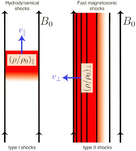
$A schematic of the orientation, propagation direction, and shock jump, ρ/ρ0, of the two shocks discussed in Section 3. Left: type I hydrodynamical shocks form from streaming material up and down ${B}_0$. Right: type II fast magnetosonic shocks that form from longitudinal compressions of the magnetic field lines. These cause longitudinal compressions in the density field because the density is flux frozen to the magnetic field.$

Figure 1.

A schematic of the orientation, propagation direction, and shock jump, ρ/ρ₀, of the two shocks discussed in Section 3. Left: type I hydrodynamical shocks form from streaming material up and down |${B}_0$|⁠. Right: type II fast magnetosonic shocks that form from longitudinal compressions of the magnetic field lines. These cause longitudinal compressions in the density field because the density is flux frozen to the magnetic field.

Open in new tab Download slide

The general form of this variance can be constructed as follows:³

$$\begin{eqnarray*} \sigma ^2_{\rho /\rho _0} = \sigma ^2_{\rho /\rho _0 \parallel } + \sigma ^2_{\rho /\rho _0 \perp } + 2\sigma _{\rho /\rho _0 \parallel }\sigma _{\rho /\rho _0 \perp }, \end{eqnarray*}$$

(15)

which decomposes the total variance into components of the density variance parallel to |${B}_0$|⁠, termed |$\sigma ^2_{\rho /\rho _0 \parallel }$|⁠, and perpendicular to |${B}_0$|⁠, termed |$\sigma ^2_{\rho /\rho _0 \perp }$|⁠. By assuming that these fluctuations are independent from one another we can further simplify the equation to

$$\begin{eqnarray*} \sigma ^2_{\rho /\rho _0} \approx \sigma ^2_{\rho /\rho _0 \parallel } + \sigma ^2_{\rho /\rho _0 \perp }, \end{eqnarray*}$$

(16)

where the correlation term, |$2\sigma _{\rho /\rho _0 \parallel }\sigma _{\rho /\rho _0 \perp }$|⁠, between the fluctuations becomes zero in the statistical average.⁴ For a short discussion on how the velocity and magnetic field is arranged in this turbulence regime, we refer the reader to Appendix A. The main purpose of this study is therefore to explore and model each of these components, extending the work of Molina et al. (2012) and Beattie & Federrath (2020) and indeed the numerous works on |$\sigma ^2_{\rho /\rho _0}$| into the sub-Alfvénic, anisotropic, supersonic turbulent regime. Furthermore, with the development of a density fluctuation model, this is the first step towards an anisotropic, magnetoturbulent star formation theory.

3 DERIVING AN ANISOTROPIC DENSITY VARIANCE MODEL

In this section, we construct an anisotropic variance model. We first explore some geometrical features of shocks, summarizing the key works of Padoan & Nordlund (2011) and Molina et al. (2012), and derive equation (14). Next we create our two-shock model for the anisotropic density field, based on hydrodynamical shocks that travel parallel to the mean magnetic field, which we call type I shocks, and fast magnetosonic shocks that travel perpendicular to the mean magnetic field, which we call type II shocks. Finally, we discuss the volume-filling fractions of the two shock types and the limiting behaviour of the model.

3.1 Geometry of a shock

Consider a planar shock with surface area |$\ell ^2_{\rm shock}$| and shock width λ, propagating in a system with volume |$\mathcal {V} = L^3$|⁠. The volume of the shock is then

$$\begin{eqnarray*} \mathcal {V}_{\text{shock}}= \lambda L^2. \end{eqnarray*}$$

(17)

The shock width is proportional to the density jump between the pre-shock (ρ₀) and post-shock (ρ₁) densities, multiplied by the integral scale of the turbulence, θL, i.e. the scale where velocity structure is no longer correlated,

$$\begin{eqnarray*} \lambda \approx \theta L \frac{\rho _0}{\rho _1}, \end{eqnarray*}$$

(18)

which is derived in Padoan & Nordlund (2011) by balancing the ram and thermal pressures for a shock in hydrodynamical turbulence. We substitute equation (18) into equation (17) to reveal the volume of the shock in terms of the density contrast,

$$\begin{eqnarray*} \mathcal {V}_{\text{shock}}\approx \theta L^3 \frac{\rho _0}{\rho _1}. \end{eqnarray*}$$

(19)

Now assuming that |$\operatorname{d}\!{\mathcal {V}} \approx \operatorname{d}\!{\mathcal {V}_{\text{shock}}}$| we can construct the volume differential, substitute it into equation (14), and integrate it to construct the variance as a function of density contrasts. Hence,⁵

$$\begin{eqnarray*} \operatorname{d}\!{\mathcal {V}} & \approx \theta L^3 \left(\frac{\rho _0}{\rho _1} \right)^2 \operatorname{d}\!{\left(\frac{\rho _1}{\rho _0}\right)}, \end{eqnarray*}$$

(20)

and therefore we can rewrite equation (14) in terms of density contrasts in the range 1 ≤ ρ₁/ρ₀ ≤ ρ/ρ₀,⁶ which is the density domain for which shocks are well defined in

$$\begin{eqnarray*} \sigma _{\rho /\rho _0}^2 &\approx \frac{1}{\mathcal {V}} \int _{1}^{\rho / \rho _0} \operatorname{d}\!{\left(\frac{\rho _1}{\rho _0}\right)} \, \mathcal {V}\theta \left(\frac{\rho _0}{\rho _1} \right)^2 \left(\frac{\rho _1}{\rho _0} - 1 \right)^2, \end{eqnarray*}$$

(21)

$$\begin{eqnarray*} &= \theta \int _{1}^{\rho / \rho _0} \operatorname{d}\!{\left(\frac{\rho _1}{\rho _0}\right)} \, \left(1 - \frac{\rho _0}{\rho _1} \right)^2, \end{eqnarray*}$$

(22)

$$\begin{eqnarray*} \frac{\sigma _{\rho /\rho _0}^2}{\theta } &\approx \underbrace{\frac{\rho }{\rho _0}}_{{\text{overdensities}}} - \overbrace{\frac{\rho _0}{\rho }}^{{\text{underdensities}}} - \underbrace{2\ln \left(\frac{\rho }{\rho _0} \right)}_{{\substack{\text{logarithmic} \\ \text{overdensities}}}}, \end{eqnarray*}$$

(23)

where |$\mathcal {V}= L^3$| cancels between the differential element of the shock and volume-weighted integral. What this means is that for a single-shock model we average over the shock-jump conditions through the whole volume of interest. This will be important for generalizing this model to multiple shocks in Section 3.3. The first term in equation (23), ρ/ρ₀, the overdensities, dominates the total variance, since the amplitude of the density fluctuations is large in supersonic turbulence. Both ρ₀/ρ, the underdensities, and ln (ρ/ρ₀), the logarithmic overdensities, are small in comparison, allowing us to approximate the total variance as solely dependent upon the overdensities (Padoan & Nordlund 2011). Assuming the integral scale factor is θ ≈ 1, i.e. of order the system scale (Federrath & Klessen 2012), and making the above approximation we find the relation

$$\begin{eqnarray*} \sigma _{\rho /\rho _0}^2 \approx \frac{\rho }{\rho _0}, \end{eqnarray*}$$

(24)

which is the key result that Padoan & Nordlund (2011) and Molina et al. (2012) use to relate the variance to the shock-jump conditions. Before generalizing this result, we first consider the details of the two shock types that we use to construct our model of the anisotropic density variance.

3.2 Shocks in MHD turbulence

We have now seen that the variance of a stochastic density field full of shocks can be related to the shock-jump conditions. The shock-jump conditions can be derived in the regular Rankine–Hugoniot fashion, where we equate the upstream and downstream |${B}$|⁠, |$\rho {v}$|⁠, and ρ (for an isothermal shock) across the shock boundary, in the local frame of the shock, to conserve energy, momentum, and mass (Landau & Lifshitz 1959), and we follow Molina et al. (2012) to include the magnetic pressure contribution in the derivation. In the following two subsections, we will describe two different types of shocks that are derived using this method.

3.2.1 Type I: hydrodynamic shocks

In isotropic, supersonic turbulence shocks are randomly oriented in space. However, in the presence of a strong mean magnetic field, where δB ≪ B₀, shocks form from velocity gradients along the magnetic field (Beattie et al. 2020). We call these shocks type I shocks. The shocks create large density contrasts perpendicular to the mean field that propagate parallel to it (Beattie & Federrath 2020). Since the propagation is parallel to |${B}_0$| the shocks do not feel the Lorentz force (nor does the magnetic field feel the shock, with upstream and downstream |${B}$| remaining unchanged), and hence the shock-jump conditions are hydrodynamical in nature (Mocz & Burkhart 2018). This is the supersonic (non-linear) equivalent of slow or acoustic modes from linearized MHD turbulence theory. For an isothermal fluid, with turbulence driving parameter b, the shock jump is

$$\begin{eqnarray*} \left(\frac{\rho }{\rho _0}\right)_{\parallel } = b^2 \mathcal {M}^2, \end{eqnarray*}$$

(25)

where |$b\mathcal {M}$| is the compressive component of the Mach number (Federrath et al. 2008; Konstandin et al. 2012b), which is the Mach number associated with the compressive modes in the flow. It follows from equation (24) that

$$\begin{eqnarray*} \sigma ^2_{\rho /\rho _0 \parallel } \approx b^2 \mathcal {M}^2. \end{eqnarray*}$$

(26)

3.2.2 Type II: fast magnetosonic shocks

Fast magnetosonic waves are the only MHD waves (in linearized MHD theory) that can propagate perpendicular to the magnetic field and compress the gas (Landau & Lifshitz 1959; Lehmann et al. 2016; Tritsis & Tassis 2016). The perpendicular waves propagate with velocity

$$\begin{eqnarray*} v = \sqrt{v_{\rm A0}^2 + c_\mathrm{ s}^2}, \end{eqnarray*}$$

(27)

where |$v_{\rm A0} = B_0 / \sqrt{4\pi \rho }$| is the mean-field Alfvén velocity, and c_s is the sound speed. The non-linear counterpart is the fast magnetosonic shock, which too propagates orthogonal to |${B}_0$|⁠. We call this a type II shock. These shocks form through longitudinal compressions of the field lines, visualized in fig. 2 of Beattie et al. (2020). The field lines compress together, causing longitudinal, striated compressions in the density field. Through the flux-freezing condition, the magnetic field is locked perpendicular to the shock with B ∝ ρ, hence these shocks are equivalent to the B ∝ ρ shocks described in Molina et al. (2012). In an isothermal fluid the gas pressure scales directly with ρ and hence the magnetic field becomes larger at higher ρ/ρ₀ in the fluid (Mocz & Burkhart 2018). The shock jump is given by

$$\begin{eqnarray*} \left(\frac{\rho }{\rho _0}\right)_{\perp } = \dfrac{1}{2}\left[\sqrt{\left(1 + 2\frac{\mathcal {M}^{2}_{\text{A0}}}{b^2\mathcal {M}^2}\right)^2 + 8\mathcal {M}^{2}_{\text{A0}}} -\left(1 + 2\frac{\mathcal {M}^{2}_{\text{A0}}}{b^2\mathcal {M}^2}\right) \right], \nonumber \\ \end{eqnarray*}$$

(28)

and hence,

$$\begin{eqnarray*} \sigma ^2_{\rho /\rho _0 \perp } \approx \dfrac{1}{2}\left[\sqrt{\left(1 + 2\frac{\mathcal {M}^{2}_{\text{A0}}}{b^2\mathcal {M}^2}\right)^2 + 8\mathcal {M}^{2}_{\text{A0}}} -\left(1 + 2\frac{\mathcal {M}^{2}_{\text{A0}}}{b^2\mathcal {M}^2}\right) \right]. \nonumber \\ \end{eqnarray*}$$

(29)

Unlike the hydrodynamical shock-jump condition in equation (25), the density jump for fast magnetosonic waves is asymptotic to |$(\rho /\rho _0)_{\perp } = (\sqrt{1 + 8\mathcal {M}^{2}_{\text{A0}}}-1)/2$| as |$\mathcal {M}\rightarrow \infty$|⁠. The limit is controlled entirely by the strength of the magnetic field. Physically, this corresponds to the strong magnetic field suppressing small-scale fluctuations that are introduced to the density as |$\mathcal {M}$| increases (i.e. steepening of the ρ power spectra; Kim & Ryu 2005; Beattie & Federrath 2020). If |$\operatorname{\mathcal {M}_{\text{A0}}}\rightarrow 0$|⁠, then (ρ/ρ₀)_⊥ → 0. This is because the divergence of the velocity field only has a parallel to |${B}_0$| component as B₀ ≫ δB, where δB is the fluctuating component of the magnetic field. Hence one cannot create any perpendicular density contrasts for B₀ → ∞ (Beattie et al. 2020).

3.3 Two-shock density variance model

Now we combine equations (26) and (29) to model the total variance of the anisotropic density field, i.e. we assume the stochastic medium of interest is composed out of the type I and type II shocks discussed above. Thus, we model the total fluctuations as the sum of integrals over the shock-jump conditions in the parallel and perpendicular directions, as discussed in Section 3.1, assuming that the fluctuations are independent from one another. In reality there will be some non-linear mixing of the shocks (e.g. type II shocks compressing the type I shocks longitudinally, changing the shock-jump conditions through a multiplicative interaction) and, in principle, a larger diversity of shocks and density fluctuations, but we adopt the most parsimonious anisotropic model for the variance that one can formulate and leave generalizations of the model for future studies. The N-shock model would sum over N types of uncorrelated shocks with shock-jump conditions (ρ/ρ₀)_i and shock volumes |$\mathcal {V}_i$|⁠, given by

$$\begin{eqnarray*} \sigma ^2_{\rho /\rho _0} = \frac{1}{\mathcal {V}} \sum _{i}^{N} \int _{\mathcal {V}_i} \operatorname{d}\!{\mathcal {V}_i} \, \left[ \left(\frac{\rho }{\rho _0}\right)_{i} - 1 \right]^2. \end{eqnarray*}$$

(30)

For our two-shock model (N = 2, for type I and type II), this leads to

$$\begin{eqnarray*} \sigma _{\rho /\rho _0}^2 &=& \sigma _{\rho /\rho _0\parallel }^2 + \sigma _{\rho /\rho _0\perp }^2= \underbrace{f_{\parallel } \int _{1}^{\rho / \rho _0} \operatorname{d}\!{\left(\frac{\rho _1}{\rho _0}\right)_{\parallel }} \, \left(\frac{\rho _1}{\rho _0} \right)^{-2}_{\parallel } \left(\frac{\rho _1}{\rho _0} - 1 \right)^2_{\parallel }}_{\sigma ^2_{\parallel }} \nonumber \\ &&+ \underbrace{f_{\perp } \int _{1}^{\rho / \rho _0} \operatorname{d}\!{\left(\frac{\rho _1}{\rho _0}\right)}_{\perp } \, \left(\frac{\rho _1}{\rho _0} \right)_{\perp }^{-2} \left(\frac{\rho _1}{\rho _0} - 1 \right)^2_{\perp }}_{\sigma ^2_{\perp }}, \end{eqnarray*}$$

(31)

$$\begin{eqnarray*} \sigma _{\rho /\rho _0}^2 = \underbrace{ f_{\parallel } b^2 \mathcal {M}^2}_{\sigma ^2_{\parallel }} + \underbrace{ \frac{f_{\perp }}{2}\left[ \sqrt{\left(1 + 2\frac{\mathcal {M}^{2}_{\text{A0}}}{b^2\mathcal {M}^2}\right)^2 + 8\mathcal {M}^{2}_{\text{A0}}} -\left(1 + 2\frac{\mathcal {M}^{2}_{\text{A0}}}{b^2\mathcal {M}^2}\right) \right]}_{\sigma ^2_{\perp }}, \nonumber \\ \end{eqnarray*}$$

(32)

where the parameters f_∥ and f_⊥ control the weighting of the contributions from each of the shock types, and come directly from integrating equation (14) over two different subvolumes that the fluctuations occupy. We call these the volume fractions of the parallel and perpendicular fluctuations, respectively, and discuss and determine f_∥ and f_⊥ in Section 5.1 below.

4 MHD SIMULATIONS

4.1 MHD model

Here we describe the numerical data that we use to test our density variance model. These are high-resolution, three-dimensional, ideal magnetohydrodynamical (MHD) simulations of supersonic turbulence. The ideal, isothermal MHD equations are

$$\begin{eqnarray*} \frac{\partial \rho }{\partial t} + \nabla \cdot (\rho {v}) &= 0 , \end{eqnarray*}$$

(33)

$$\begin{eqnarray*} \rho \left(\frac{\partial }{\partial t} + {v}\cdot \nabla \right) {v} &= \frac{({B} \cdot \nabla){B}}{4\pi } - \nabla \left(c_\mathrm{ s}^2 \rho + \frac{|{B}|^2}{8\pi }\right) + \rho {F}, \end{eqnarray*}$$

(34)

$$\begin{eqnarray*} \frac{\partial {B}}{\partial t} &= \nabla \times ({v} \times {B}), \end{eqnarray*}$$

(35)

$$\begin{eqnarray*} \nabla \cdot {B} &= 0, \end{eqnarray*}$$

(36)

where |${v}$| is the fluid velocity, ρ the density, |${B}$| the magnetic field, c_s the sound speed, and |${F}$| a stochastic function that drives the turbulence. We use a modified version of flash based on version 4.0.1 (Fryxell et al. 2000; Dubey et al. 2008) to solve the MHD equations in a periodic box with dimensions L³, on a uniform grid with resolution 512³, using the multiwave, approximate Riemann solver framework described in Bouchut, Klingenberg & Waagan (2010) and implemented in flash by Waagan, Federrath & Klingenberg (2011). For a detailed discussion of the simulations we refer the reader to Beattie & Federrath (2020) and Beattie et al. (2020). Table 1 provides a summary of the important time-averaged parameter values. Here we briefly summarize the key methods and properties of the simulations.

Table 1.

Open in new tab

Main simulation parameters.

Sim. ID	\|$\mathcal {M}\, (\pm 1\sigma)$\|	\|$\operatorname{\mathcal {M}_{\text{A0}}}\, (\pm 1\sigma)$\|	\|$\sigma _{\rho /\rho _0}^2\, (\pm 1\sigma)$\|	N³
(1)	(2)	(3)	(4)	(5)
M2Ma0.1	2.6 ± 0.2	0.131 ± 0.008	0.49 ± 0.05	512³
M4Ma0.1	5.2 ± 0.4	0.13 ± 0.01	1.6 ± 0.3	512³
M10Ma0.1	12 ± 1	0.125 ± 0.006	5.3 ± 0.9	512³
M20Ma0.1	24 ± 1	0.119 ± 0.003	7 ± 1	512³
M2Ma0.5	2.2 ± 0.2	0.54 ± 0.04	0.51 ± 0.07	512³
M4Ma0.5	4.4 ± 0.2	0.54 ± 0.03	1.8 ± 0.3	512³
M10Ma0.5	10.5 ± 0.5	0.52 ± 0.02	5.1 ± 0.7	512³
M20Ma0.5	21 ± 1	0.53 ± 0.02	8 ± 1	512³
M2Ma1.0	2.0 ± 0.1	0.98 ± 0.07	0.5 ± 0.1	512³
M4Ma1.0	3.8 ± 0.3	0.95 ± 0.08	2.0 ± 0.3	512³
M10Ma1.0	9.3 ± 0.5	0.93 ± 0.05	8 ± 1	512³
M20Ma1.0	18.8 ± 0.7	0.93 ± 0.03	12 ± 2	512³

Sim. ID	\|$\mathcal {M}\, (\pm 1\sigma)$\|	\|$\operatorname{\mathcal {M}_{\text{A0}}}\, (\pm 1\sigma)$\|	\|$\sigma _{\rho /\rho _0}^2\, (\pm 1\sigma)$\|	N³
(1)	(2)	(3)	(4)	(5)
M2Ma0.1	2.6 ± 0.2	0.131 ± 0.008	0.49 ± 0.05	512³
M4Ma0.1	5.2 ± 0.4	0.13 ± 0.01	1.6 ± 0.3	512³
M10Ma0.1	12 ± 1	0.125 ± 0.006	5.3 ± 0.9	512³
M20Ma0.1	24 ± 1	0.119 ± 0.003	7 ± 1	512³
M2Ma0.5	2.2 ± 0.2	0.54 ± 0.04	0.51 ± 0.07	512³
M4Ma0.5	4.4 ± 0.2	0.54 ± 0.03	1.8 ± 0.3	512³
M10Ma0.5	10.5 ± 0.5	0.52 ± 0.02	5.1 ± 0.7	512³
M20Ma0.5	21 ± 1	0.53 ± 0.02	8 ± 1	512³
M2Ma1.0	2.0 ± 0.1	0.98 ± 0.07	0.5 ± 0.1	512³
M4Ma1.0	3.8 ± 0.3	0.95 ± 0.08	2.0 ± 0.3	512³
M10Ma1.0	9.3 ± 0.5	0.93 ± 0.05	8 ± 1	512³
M20Ma1.0	18.8 ± 0.7	0.93 ± 0.03	12 ± 2	512³

Note. For each simulation we extract 51 realizations at times |$t/T\in \left\lbrace 5.0,\, 5.1, \ldots , 10.0\right\rbrace$|⁠, where T is the turbulent turnover time, and all 1σ fluctuations listed are from the time-averaging over the |$5\, T$| time span. Column (1): the simulation ID. Column (2): the rms turbulent Mach number, |$\mathcal {M}= \sigma _V / c_\mathrm{ s}$|⁠. Column (3): the Alfvén Mach number for the mean-|${B}$| component, |${B}_0$|⁠, |$\operatorname{\mathcal {M}_{\text{A0}}}= (2c_\mathrm{ s}\mathcal {M}\sqrt{\pi \rho _0}) / |{B}_0|$|⁠, where ρ₀ is the mean density and c_s is the sound speed. Column (4): the volume-weighted density variance, computed as shown in equation (14). Column (5): the number of computational cells for the discretization of the spatial domain of size L³.

Table 1.

Open in new tab

Main simulation parameters.

Sim. ID	\|$\mathcal {M}\, (\pm 1\sigma)$\|	\|$\operatorname{\mathcal {M}_{\text{A0}}}\, (\pm 1\sigma)$\|	\|$\sigma _{\rho /\rho _0}^2\, (\pm 1\sigma)$\|	N³
(1)	(2)	(3)	(4)	(5)
M2Ma0.1	2.6 ± 0.2	0.131 ± 0.008	0.49 ± 0.05	512³
M4Ma0.1	5.2 ± 0.4	0.13 ± 0.01	1.6 ± 0.3	512³
M10Ma0.1	12 ± 1	0.125 ± 0.006	5.3 ± 0.9	512³
M20Ma0.1	24 ± 1	0.119 ± 0.003	7 ± 1	512³
M2Ma0.5	2.2 ± 0.2	0.54 ± 0.04	0.51 ± 0.07	512³
M4Ma0.5	4.4 ± 0.2	0.54 ± 0.03	1.8 ± 0.3	512³
M10Ma0.5	10.5 ± 0.5	0.52 ± 0.02	5.1 ± 0.7	512³
M20Ma0.5	21 ± 1	0.53 ± 0.02	8 ± 1	512³
M2Ma1.0	2.0 ± 0.1	0.98 ± 0.07	0.5 ± 0.1	512³
M4Ma1.0	3.8 ± 0.3	0.95 ± 0.08	2.0 ± 0.3	512³
M10Ma1.0	9.3 ± 0.5	0.93 ± 0.05	8 ± 1	512³
M20Ma1.0	18.8 ± 0.7	0.93 ± 0.03	12 ± 2	512³

Sim. ID	\|$\mathcal {M}\, (\pm 1\sigma)$\|	\|$\operatorname{\mathcal {M}_{\text{A0}}}\, (\pm 1\sigma)$\|	\|$\sigma _{\rho /\rho _0}^2\, (\pm 1\sigma)$\|	N³
(1)	(2)	(3)	(4)	(5)
M2Ma0.1	2.6 ± 0.2	0.131 ± 0.008	0.49 ± 0.05	512³
M4Ma0.1	5.2 ± 0.4	0.13 ± 0.01	1.6 ± 0.3	512³
M10Ma0.1	12 ± 1	0.125 ± 0.006	5.3 ± 0.9	512³
M20Ma0.1	24 ± 1	0.119 ± 0.003	7 ± 1	512³
M2Ma0.5	2.2 ± 0.2	0.54 ± 0.04	0.51 ± 0.07	512³
M4Ma0.5	4.4 ± 0.2	0.54 ± 0.03	1.8 ± 0.3	512³
M10Ma0.5	10.5 ± 0.5	0.52 ± 0.02	5.1 ± 0.7	512³
M20Ma0.5	21 ± 1	0.53 ± 0.02	8 ± 1	512³
M2Ma1.0	2.0 ± 0.1	0.98 ± 0.07	0.5 ± 0.1	512³
M4Ma1.0	3.8 ± 0.3	0.95 ± 0.08	2.0 ± 0.3	512³
M10Ma1.0	9.3 ± 0.5	0.93 ± 0.05	8 ± 1	512³
M20Ma1.0	18.8 ± 0.7	0.93 ± 0.03	12 ± 2	512³

Note. For each simulation we extract 51 realizations at times |$t/T\in \left\lbrace 5.0,\, 5.1, \ldots , 10.0\right\rbrace$|⁠, where T is the turbulent turnover time, and all 1σ fluctuations listed are from the time-averaging over the |$5\, T$| time span. Column (1): the simulation ID. Column (2): the rms turbulent Mach number, |$\mathcal {M}= \sigma _V / c_\mathrm{ s}$|⁠. Column (3): the Alfvén Mach number for the mean-|${B}$| component, |${B}_0$|⁠, |$\operatorname{\mathcal {M}_{\text{A0}}}= (2c_\mathrm{ s}\mathcal {M}\sqrt{\pi \rho _0}) / |{B}_0|$|⁠, where ρ₀ is the mean density and c_s is the sound speed. Column (4): the volume-weighted density variance, computed as shown in equation (14). Column (5): the number of computational cells for the discretization of the spatial domain of size L³.

In Fig. 2, we show the time-averaged logarithmic density PDFs for the |$\operatorname{\mathcal {M}_{\text{A0}}}= 0.1$| simulations shown in Table 1. We show a lognormal model fit to the density fluctuations with dotted lines. The density PDFs show that the fluctuations are well described by a lognormal model, especially as |$\mathcal {M}$| increases. This is in contrast with hydrodynamical and super-Alfvénic compressible turbulent flows, which become less lognormal as the |$\mathcal {M}$| increases (Federrath et al. 2010; Hopkins 2013b; Mocz & Burkhart 2019). We leave the detailed analysis of the Gaussianity of the density PDFs for a follow-up study, but stress that in the sub-Alfvénic regime the variance of the density field, which is the focus of this study, is an informative statistic because of the lognormal fluctuations.

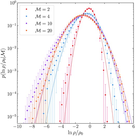
$Time-averaged logarithmic density PDFs for the ensemble of simulations, $2 \lesssim \mathcal {M}\lesssim 20$ with $\operatorname{\mathcal {M}_{\text{A0}}}= 0.1$. We show lognormal curves overlaid with dotted lines on the data. Consistent with findings in Molina et al. (2012), for sub-Alfvénic mean-field compressible turbulence we find that the density fluctuations are approximately lognormal, and do not exhibit strong skewness features that are present in hydrodynamical turbulence (Federrath et al. 2010; Hopkins 2013b; Mocz & Burkhart 2019), and hence are well described by the variance of the density field.$

Figure 2.

Time-averaged logarithmic density PDFs for the ensemble of simulations, |$2 \lesssim \mathcal {M}\lesssim 20$| with |$\operatorname{\mathcal {M}_{\text{A0}}}= 0.1$|⁠. We show lognormal curves overlaid with dotted lines on the data. Consistent with findings in Molina et al. (2012), for sub-Alfvénic mean-field compressible turbulence we find that the density fluctuations are approximately lognormal, and do not exhibit strong skewness features that are present in hydrodynamical turbulence (Federrath et al. 2010; Hopkins 2013b; Mocz & Burkhart 2019), and hence are well described by the variance of the density field.

Open in new tab Download slide

4.2 Turbulent driving, density and velocity fields

The initial velocity field is set to |${v}(x,y,z,t=0)={0}$|⁠, with units c_s = 1, and the density field ρ(x, y, z, t = 0) = ρ₀, with units ρ₀ = 1. The turbulent acceleration field, |${F}$|⁠, in equation (34) follows an Ornstein–Uhlenbeck process in time and is constructed such that we can control the mixture of solenoidal and compressive modes in |${F}$| (see Federrath et al. 2008, 2009, 2010 for a detailed discussion of the turbulence driving). We choose to drive with a natural mixture of the two modes (Federrath et al. 2010), which corresponds to b ≈ 0.4. We isotropically drive in wavenumber space, centred on k = 2, corresponding to real-space scales of ℓ_D = L/2, and falling off to zero with a parabolic spectrum between k = 1 and k = 3. Thus, energy is injected only on large scales and the turbulence on smaller scales develops self-consistently through the MHD equations. The autocorrelation time-scale of |${F}$| is equal to

$$\begin{eqnarray*} T = \frac{\ell _\mathrm{ D}}{\sigma _V} = \frac{L}{2 c_\mathrm{ s} \mathcal {M}}. \end{eqnarray*}$$

(37)

We vary the sonic Mach number between |$\mathcal {M}= 2$| and 20, encapsulating the range of observed |$\mathcal {M}$| values for turbulent MCs (e.g. Schneider et al. 2013; Federrath et al. 2016; Orkisz et al. 2017; Beattie et al. 2019b). We run the simulations from 0 ≤ t/T ≤ 10 and extract 51 time realizations of ρ(x, y, z) over 5 ≤ t/T ≤ 10 to gather data only when the turbulence is in a statistically stationary state (Federrath et al. 2009; Price & Federrath 2010). For simulations with a strong guide field, a statistically steady state is reached after about 5T, while for purely hydrodynamical turbulence and super-Afvénic turbulence, stationarity is already reached after about 2T. All our results are based on time-averages across these 51 realizations, unless explicitly indicated otherwise.

In Fig. 3, we show density slices through a plane perpendicular to the direction of |${B}_0$|⁠, indicated in the top left-hand plot. The plots are organized such that the top left-hand plot has the weakest (but still supersonic) turbulence (⁠|$\mathcal {M}= 2$|⁠) and strongest B₀ (⁠|$\operatorname{\mathcal {M}_{\text{A0}}}= 0.1$|⁠), and the bottom right-hand plot has the strongest turbulence (⁠|$\mathcal {M}= 20$|⁠) and weakest B₀ (⁠|$\operatorname{\mathcal {M}_{\text{A0}}}= 1.0$|⁠). The slices reveal the highly anisotropic density structures that form in sub-Alfvénic, supersonic turbulence. Overdensities and rarefactions from fast magnetosonic shocks (type II shocks) cause ripples through the density running parallel to the magnetic field. The largest density contrasts are from the shocks that form along the magnetic field (type I shocks), which compress the gas density into sharp, fractal filaments. The filamentary structures become less space filling as |$\mathcal {M}$| increases, extending across |$\propto L/\mathcal {M}^2 \propto L/4$| for |$\mathcal {M}\approx 2$|⁠, to a tiny fraction of the box at |$\mathcal {M}\approx 20$|⁠, qualitatively consistent with the shock-width model discussed in Section 3.1.

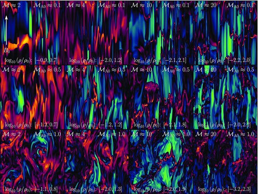
$Slices through the y = 0 plane of log10(ρ/ρ0) at $t = 6\, T$ for the 12 simulations listed in Table 1. The mean magnetic field, ${B}_0$, is oriented up the page as shown in the top left-hand panel. The plots are ordered such that the simulations with the highest Mach numbers are on the right-hand column ($\mathcal {M}\approx 20$) and weakest ($\mathcal {M}\approx 2$) on the left-hand column. Likewise, the strongest B0 simulations $(\operatorname{\mathcal {M}_{\text{A0}}}\approx 0.1)$ are on the top row and weakest ($\operatorname{\mathcal {M}_{\text{A0}}}\approx 1.0$) on the bottom row. The top row reveals slices of the density structures for the most anisotropic simulations. For these simulations, fast magnetosonic waves (type II shocks, Section 3.2.2) ripple through the density field, propagating perpendicular to ${B}_0$ and leaving striations from the compressions (ρ/ρ0 > 1, shown in orange) and rarefactions (ρ/ρ0 < 1, shown in green) in the field. The largest overdensities however form along the ${B}_0$, which are space filling for low-$\mathcal {M}$, and narrow and highly compressed for high-$\mathcal {M}$ (type I shocks, Section 3.2.1). For the $\operatorname{\mathcal {M}_{\text{A0}}}= 1.0$ simulations the anisotropy is beginning to weaken as the fluctuating component of the magnetic field grows, and becomes mixed into the fluid through the turbulence.$

Figure 3.

Slices through the y = 0 plane of log₁₀(ρ/ρ₀) at |$t = 6\, T$| for the 12 simulations listed in Table 1. The mean magnetic field, |${B}_0$|⁠, is oriented up the page as shown in the top left-hand panel. The plots are ordered such that the simulations with the highest Mach numbers are on the right-hand column (⁠|$\mathcal {M}\approx 20$|⁠) and weakest (⁠|$\mathcal {M}\approx 2$|⁠) on the left-hand column. Likewise, the strongest B₀ simulations |$(\operatorname{\mathcal {M}_{\text{A0}}}\approx 0.1)$| are on the top row and weakest (⁠|$\operatorname{\mathcal {M}_{\text{A0}}}\approx 1.0$|⁠) on the bottom row. The top row reveals slices of the density structures for the most anisotropic simulations. For these simulations, fast magnetosonic waves (type II shocks, Section 3.2.2) ripple through the density field, propagating perpendicular to |${B}_0$| and leaving striations from the compressions (ρ/ρ₀ > 1, shown in orange) and rarefactions (ρ/ρ₀ < 1, shown in green) in the field. The largest overdensities however form along the |${B}_0$|⁠, which are space filling for low-|$\mathcal {M}$|⁠, and narrow and highly compressed for high-|$\mathcal {M}$| (type I shocks, Section 3.2.1). For the |$\operatorname{\mathcal {M}_{\text{A0}}}= 1.0$| simulations the anisotropy is beginning to weaken as the fluctuating component of the magnetic field grows, and becomes mixed into the fluid through the turbulence.

Open in new tab Download slide

Using the ospray ray tracer in visit (Childs et al. 2012) we show examples of the volumetric density field for the M2MA0.1 and M20MA0.1 simulations in Fig. 4. Large-scale vortices are revealed in the M2MA0.1 simulation, with sheets of density wrapped around in the direction of the |${B}_0$|⁠. The vortices form at roughly the driving scale (L/2) of the simulation. The volumetric rendering for M20MA0.1 shows much more small-scale structure compared to M2MA0.1, both along and perpendicular to the direction of |${B}_0$|⁠. The large-scale vortices found in M2MA0.1 are roughly at the same scale as the vortices in M20MA0.1, suggesting that it is the driving scale that sets the size of the vortices. Dense, shocked material is compressed along the magnetic field lines, creating the filamentary structures that were found in the slices, oriented perpendicular to the field.

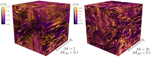
$The structure of the 3D density field, ρ/ρ0, for the highly magnetized M2MA0.1 (left) and M20MA0.1 (right) simulations (see Table 1). The direction of the mean magnetic field, ${B}_0$, is shown at the bottom right-hand corner of the simulations. Large-scale vortices form in the density plane perpendicular to ${B}_0$. Density structures are tightly wound and stretched into ribbons and tubes as the supersonic vortices advect the flux-frozen density field around the field lines. The vortices are found on similar scales for both simulations, roughly L/2, the driving scale of the turbulence, however the M20MA0.1 simulation has more small-scale density fluctuations than the M2MA0.1 simulation (note the different scaling of the colour bars).$

Figure 4.

The structure of the 3D density field, ρ/ρ₀, for the highly magnetized M2MA0.1 (left) and M20MA0.1 (right) simulations (see Table 1). The direction of the mean magnetic field, |${B}_0$|⁠, is shown at the bottom right-hand corner of the simulations. Large-scale vortices form in the density plane perpendicular to |${B}_0$|⁠. Density structures are tightly wound and stretched into ribbons and tubes as the supersonic vortices advect the flux-frozen density field around the field lines. The vortices are found on similar scales for both simulations, roughly L/2, the driving scale of the turbulence, however the M20MA0.1 simulation has more small-scale density fluctuations than the M2MA0.1 simulation (note the different scaling of the colour bars).

Open in new tab Download slide

4.3 Magnetic fields

The initial magnetic field, |${B}(x,y,z) = B_0\hat{{z}}$| at t = 0, in equations (34)–(36) is a uniform field with field lines threaded through the |$\hat{{z}}$| direction of the simulations. B₀ is set to ensure the desired |$\operatorname{\mathcal {M}_{\text{A0}}}$|⁠, using the definition of the Alfvén velocity (see footnote⁷) and the turbulent Mach number (see equation 5),

$$\begin{eqnarray*} \operatorname{\mathcal {M}_{\text{A0}}}= \sigma _V / V_{\rm A0} = 2c_\mathrm{ s}\sqrt{\pi \rho _0}\mathcal {M}/B_0, \end{eqnarray*}$$

(38)

with B₀ constant in space and time. We set |$\operatorname{\mathcal {M}_{\text{A0}}}= 0.1, \ 0.5$|⁠, and 1.0 for different simulations (see Table 1), ensuring that the turbulence is in an anisotropic regime (Beattie & Federrath 2020; Beattie et al. 2020). The total magnetic field is given by

$$\begin{eqnarray*} {B}(t) = B_0 { \hat{z}} + \delta {B}(t), \end{eqnarray*}$$

(39)

where the fluctuating component of the field, |$\delta {B}$|⁠, evolves self-consistently from the MHD equations, with |$\mathrm{\left\langle \delta {B} \right\rangle }_t = 0$|⁠. From previous experiments in the anisotropic regime discussed throughout this study, |$|\delta {B}|/|{B}_0| \approx 10^{-3} \!-\!10^{-2}$| (Federrath 2016a; Beattie et al. 2020). For this reason |$\operatorname{\mathcal {M}_{\text{A}}}\approx \operatorname{\mathcal {M}_{\text{A0}}}$| in this regime, however, we explicitly formulate our models around |$\operatorname{\mathcal {M}_{\text{A0}}}$|⁠, which is an invariant across different |$\mathcal {M}$| simulations.

5 IMPLEMENTATION OF THE ANISOTROPIC DENSITY VARIANCE MODEL

In this section, we describe and model the fluctuation volume-filling fractions that we introduced in equation (32).

5.1 Volume fractions of anisotropic fluctuations

The fluctuation volume fractions, f_∥ and f_⊥ in equation (32), determine the contributions of the parallel and perpendicular fluctuations in our model. These parameters naturally come about from considering multiple terms of a volume-weighted statistic, where the total volume is partitioned into distinct subvolumes for the parallel and perpendicular fluctuations. The volume-filling fractions can be derived by returning to equation (17), but instead of using a planar shock, we consider shocks that have a reduced volume-filling factor, f_i,

$$\begin{eqnarray*} \mathcal {V}_{{\rm shock}, i} = f_{i}\lambda L^{2}, \end{eqnarray*}$$

(40)

where i ∈ {∥, ⊥} is the volume-filling factor of the shock, e.g. for f_i = 1 the shock is the planar shock from equation (17), and for f_i < 1 the shock has a smaller volume than a planar shock, which could be, for example, a tubular, filamentary shock. Considering shocks with a variable volume is an important consideration to make in our two-shock model, because the amount of volume that the fluctuations fill encodes how much they contribute to the variance through the density variance integral, equation (14). Propagating equation (40) through equations (20)–(24), making the same assumptions but for non-planar shocks, shows that

$$\begin{eqnarray*} \sigma _{\rho /\rho _0}^2 \approx & f_{\parallel } \left[ \left(\frac{\rho }{\rho _0}\right)_{\parallel } - \left(\frac{\rho _0}{\rho }\right)_{\parallel } - 2\ln \left(\frac{\rho }{\rho _0} \right)_{\parallel }\right] \end{eqnarray*}$$

(41)

$$\begin{eqnarray*} &+ f_{\perp }\left[\left(\frac{\rho }{\rho _0}\right)_{\perp } - \left(\frac{\rho _0}{\rho }\right)_{\perp } - 2\ln \left(\frac{\rho }{\rho _0} \right)_{\perp }\right], \end{eqnarray*}$$

(42)

where f_∥ is the volume-filling fraction of the type I shocks and f_⊥ is the volume fraction of the type II shocks. Note that the geometry of the volume variable shock propagates through to the total volume fraction of the parallel and perpendicular fluctuations, including the rarefactions. This is because the rarefaction region in the flow will share some of the same geometrical properties as the shock, since the gas density is compressed from the rarefaction into the overdensity. However, as we discussed in Section 3.1, the main contributors to the variance are the overdensities, hence,

$$\begin{eqnarray*} \sigma _{\rho /\rho _0}^2 \approx & f_{\parallel } \left(\frac{\rho }{\rho _0}\right)_{\parallel } + f_{\perp } \left(\frac{\rho }{\rho _0}\right)_{\perp }, \end{eqnarray*}$$

(43)

and equation (32) immediately follows by substituting in the appropriate shock-jump conditions. Since the volume-filling fractions are for the total parallel and perpendicular fluctuations we assume that they add to unity,

$$\begin{eqnarray*} 1 = \sum _{i}^{N} f_i \iff 1 = f_{\parallel } + f_{\perp }. \end{eqnarray*}$$

(44)

This means our model is an N − 1 parameter model, where N is the number of shock types, and more explicitly, a one-parameter model for the two-shock model we describe here.

The volume-filling fractions need not be constants, and indeed, may depend upon both |$\mathcal {M}$| and |$\operatorname{\mathcal {M}_{\text{A0}}}$|⁠. For example, Konstandin et al. (2016), Beattie, Federrath & Klessen (2019a), and Beattie et al. (2019b) demonstrate that the global fractal dimension |$\mathcal {D}$|⁠, which is a measure of the how the most singular structures in the flow fill space, for supersonic turbulence depends upon |$\mathcal {M}$|⁠, which varies between 3 (space-filling, low-|$\mathcal {M}$|⁠) and 1 (filaments and tubular shocks, high-|$\mathcal {M}$|⁠). This is because the flow is more compressible for higher |$\mathcal {M}$|⁠, reducing |$\mathcal {D}$|⁠, which corresponds to the emergence of highly compressed structures like one-dimensional filaments. Increasing |$\mathcal {M}$| also directly affects the geometry of the shocks in the flow, which can be shown by expressing equation (18), the shock thickness, in terms of the shock-jump conditions for an isothermal, hydrodynamical shocks in pressure equilibrium with the ambient environment,

$$\begin{eqnarray*} \lambda \approx \frac{L}{\mathcal {M}^2}. \end{eqnarray*}$$

(45)

This establishes that the shocks become more compressed (thinner), filling less space, as |$\mathcal {M}$| increases, which means that a reasonable model for the volume fraction of the parallel fluctuations, which is dominated by type I shocks is |$f_{\parallel }\propto \mathcal {M}^{-2}$|⁠. However, this only holds for |$\mathcal {M}\gg 1$|⁠, but not for |$\mathcal {M}\sim 1$|⁠. Thus, we require a phenomenological function for the volume fraction that describes its dependence on |$\mathcal {M}$| for both the trans- to supersonic flow regime. We consider the form

$$\begin{eqnarray*} f_{\parallel } = f_0\left[1 + \left(\frac{\mathcal {M}}{\mathcal {M}_{\rm c}}\right)^4 \right]^{-1/2}, \end{eqnarray*}$$

(46)

which describes a function that tends towards |${\sim} 1/\mathcal {M}^2$| when |$\mathcal {M}\gt \mathcal {M}_{\rm c} \gg 1$| and a constant volume fraction, f₀, for |$\mathcal {M}\lt \mathcal {M}_{\rm c}$|⁠, e.g. in the subtransonic regime, where the type I shock thickness becomes ill-defined, and linear MHD waves (slow, parallel and fast, perpendicular modes) weakly compress the flow. Here, |$\mathcal {M}_{\rm c}$| defines a critical Mach number for the transition between the constant and the |${\sim} \mathcal {M}^{-2}$| regime. Thus, the parameter f₀ defines the volume-filling fraction of the parallel fluctuations, in the presence of overdensities formed by slow modes, as discussed in Section 3.2.1. These are acoustic modes that propagate along the magnetic field in the subsonic regime (Landau & Lifshitz 1959). Note that since we have assumed f_⊥ = 1 − f_∥, we only need to consider a model for f_∥.

5.2 Determining the volume fraction of parallel and perpendicular fluctuations

The first step to fitting our model is to develop a data set, (⁠|$\mathcal {M}_i,f_{\parallel ,i}$|⁠), for the different |$\operatorname{\mathcal {M}_{\text{A0}}}$| simulation listed in Table 1. Since, as discussed in Section 5.1, our model only has a single parameter, f_∥, we can rearrange equation (32) and solve analytically,⁸

$$\begin{eqnarray*} f_{\parallel } = \frac{\sigma ^2_{\rho /\rho _0} - \sigma ^2_{\rho /\rho _0\perp }}{\sigma ^2_{\rho /\rho _0\parallel } - \sigma ^2_{\rho /\rho _0\perp }}, \end{eqnarray*}$$

(47)

with the single constraint that f_∥ ∈ [0, 1], since it corresponds to a fraction of the total volume. This allows us to generate a function |$f_{\parallel }(\mathcal {M})$| for each simulation. We show this data in Fig. 5. We then fit the functional form for |$f_{\parallel }(\mathcal {M})$|⁠, equation (46), with parameters f₀ and |$\mathcal {M}_{\rm c}$| using a non-linear least-squares fitting routine weighted by |$1/\Delta f_{\parallel }^2$|⁠, where Δf_∥ is the uncertainty in f_∥, propagated through equation (47). We show the fits using the solid lines, coloured by |$\operatorname{\mathcal {M}_{\text{A0}}}$|⁠.

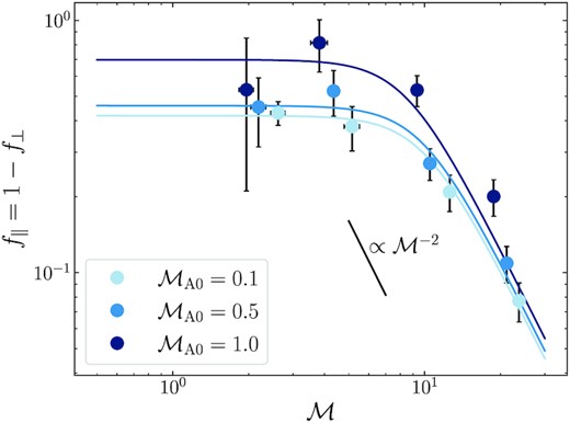
$The volume-filling fraction of fluctuations that run parallel to ${B}_0$, f∥, as a function of $\mathcal {M}$, as discussed in Section 5.1, for all of the trans-/sub-Alfvénic simulations from Table 1, with 1σ uncertainties propagated from equation (47). We fit our phenomenological models in equation (46) to each of the $\operatorname{\mathcal {M}_{\text{A0}}}$ data sets, shown with the solid lines. This model suggests that $f_{\parallel } \sim \lambda \sim \mathcal {M}^{-2}$ in the high-$\mathcal {M}$ limit, where λ is the shock width, and f∥ ∼ const. in the low-$\mathcal {M}$ limit, which is supported well by the data. This means, assuming f⊥ = 1 − f∥, f⊥ ≫ f∥ for high-$\mathcal {M}$ flows, i.e. the perpendicular fluctuations, which are dominated by fast magnetosonic shocks, contribute most to volume fraction at high-$\mathcal {M}$, which is visualized in Fig. 6.$

Figure 5.

The volume-filling fraction of fluctuations that run parallel to |${B}_0$|⁠, f_∥, as a function of |$\mathcal {M}$|⁠, as discussed in Section 5.1, for all of the trans-/sub-Alfvénic simulations from Table 1, with 1σ uncertainties propagated from equation (47). We fit our phenomenological models in equation (46) to each of the |$\operatorname{\mathcal {M}_{\text{A0}}}$| data sets, shown with the solid lines. This model suggests that |$f_{\parallel } \sim \lambda \sim \mathcal {M}^{-2}$| in the high-|$\mathcal {M}$| limit, where λ is the shock width, and f_∥ ∼ const. in the low-|$\mathcal {M}$| limit, which is supported well by the data. This means, assuming f_⊥ = 1 − f_∥, f_⊥ ≫ f_∥ for high-|$\mathcal {M}$| flows, i.e. the perpendicular fluctuations, which are dominated by fast magnetosonic shocks, contribute most to volume fraction at high-|$\mathcal {M}$|⁠, which is visualized in Fig. 6.

Open in new tab Download slide

For each of the data sets, the critical sonic Mach number is |$\mathcal {M}_{\rm c} \approx 10$| and the f₀ parameter varies monotonically between ≈0.4 and 0.7, listed in Table 2. There are two important conclusions to make: (1) magnetized turbulence is significantly saturated with shocks above |$\mathcal {M}\approx 10$|⁠; and (2) the parallel fluctuations become less confined by the magnetic field, and occupy more of the total volume when the magnetic field is weakened. Accordingly, one should expect that f₀ ∼ 1.0 as |$\operatorname{\mathcal {M}_{\text{A0}}}\rightarrow \infty$|⁠, i.e. when there is no confinement from the magnetic field. This reclaims the hydrodynamical |$\sigma _{\rho /\rho _0}^2 \!-\! \mathcal {M}$| relation. Regardless of the field strength, the high-|$\mathcal {M}$| behaviour is the same between the simulations, which is expected since the shock width, |$\lambda \sim \mathcal {M}^{-2}$|⁠, encodes how the |$(b\mathcal {M})^2$| term contributes to the total variance once the fluid is sufficiently shocked. This transition is consistent with what Beattie & Federrath (2020) found, where |$\mathcal {M}\approx 4 \!-\! 10$| marked the Mach number for when the anisotropy of the 2D power spectrum revealed a morphology dominated by shocks aligned perpendicular to |${B}_0$|⁠. Since we have assumed f_⊥ = 1 − f_∥ (equation 44) as |$\mathcal {M}$| grows and the parallel fluctuations occupy less and less of the volume until the perpendicular fluctuations contribute the most to the total volume budget for the fluid.

Table 2.

Open in new tab

Fit parameters for |$f_{\parallel }(\mathcal {M})$|⁠, as per equation (46).

Parameter	\|$\operatorname{\mathcal {M}_{\text{A0}}}=0.1$\|	\|$\operatorname{\mathcal {M}_{\text{A0}}}= 0.5$\|	\|$\operatorname{\mathcal {M}_{\text{A0}}}=1.0$\|
(1)	(2)	(3)	(4)
f₀	0.42 ± 0.05	0.46 ± 0.07	0.71 ± 0.08
\|$\mathcal {M}_{\rm c}$\|	9.9 ± 0.2	10 ± 1	10 ± 1

Parameter	\|$\operatorname{\mathcal {M}_{\text{A0}}}=0.1$\|	\|$\operatorname{\mathcal {M}_{\text{A0}}}= 0.5$\|	\|$\operatorname{\mathcal {M}_{\text{A0}}}=1.0$\|
(1)	(2)	(3)	(4)
f₀	0.42 ± 0.05	0.46 ± 0.07	0.71 ± 0.08
\|$\mathcal {M}_{\rm c}$\|	9.9 ± 0.2	10 ± 1	10 ± 1

Table 2.

Open in new tab

Fit parameters for |$f_{\parallel }(\mathcal {M})$|⁠, as per equation (46).

Parameter	\|$\operatorname{\mathcal {M}_{\text{A0}}}=0.1$\|	\|$\operatorname{\mathcal {M}_{\text{A0}}}= 0.5$\|	\|$\operatorname{\mathcal {M}_{\text{A0}}}=1.0$\|
(1)	(2)	(3)	(4)
f₀	0.42 ± 0.05	0.46 ± 0.07	0.71 ± 0.08
\|$\mathcal {M}_{\rm c}$\|	9.9 ± 0.2	10 ± 1	10 ± 1

Parameter	\|$\operatorname{\mathcal {M}_{\text{A0}}}=0.1$\|	\|$\operatorname{\mathcal {M}_{\text{A0}}}= 0.5$\|	\|$\operatorname{\mathcal {M}_{\text{A0}}}=1.0$\|
(1)	(2)	(3)	(4)
f₀	0.42 ± 0.05	0.46 ± 0.07	0.71 ± 0.08
\|$\mathcal {M}_{\rm c}$\|	9.9 ± 0.2	10 ± 1	10 ± 1

We show some of the shocked regions for both the parallel and perpendicular fluctuations in the top panels of Fig. 6, for |$\mathcal {M}\approx 20$| turbulence by taking the divergence along and across |${B}_0$|⁠. We also show the corresponding density fluctuations in the bottom two panels of the figure, where we highlight the |${-}\nabla \cdot {v} \gt 0$| regions. We find that the relative fraction of the volume occupied by type I (left-hand panel) and type II (right-hand panel) shocks is qualitatively consistent with our model, as demonstrated by the regions of high compression quantified by |${-}\nabla \cdot {v} \gt 0$| in the top panels, and corresponding density structures coloured in the bottom panels. This figure is primarily for illustrative purposes of type I and type II shocks and their approximate volume filling fractions.

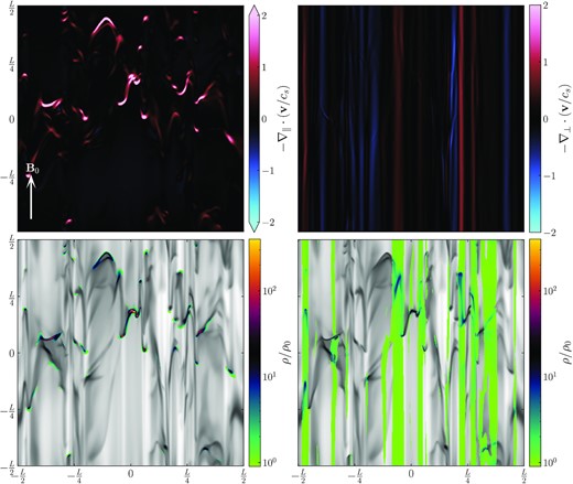
$Top left: a slice of the parallel convergence of the velocity field, with respect to the direction parallel to ${B}_0$. The convergence is in units of cs/L. Here we show a single time realization from the $\mathcal {M}= 20$, $\operatorname{\mathcal {M}_{\text{A0}}}= 0.1$ simulation (listed in Table 1), revealing hydrodynamical shocks that propagate parallel to ${B}_0$, reminiscent in morphology of the hydrodynamical bow shocks studied in Robertson & Goldreich (2018). Top right: the same time realization as the left-hand plot, but for the perpendicular convergence of the velocity field, showing fast magnetosonic compressions of the velocity field, propagating orthogonal to ${B}_0$. The amplitude of the convergence is an order of magnitude larger for the hydrodynamical shocks compared to the magnetosonic fast shocks due to the strong magnetic cushioning effect perpendicular to ${B}_0$ (Molina et al. 2012). Bottom left: the parallel shocks in the density field, corresponding to the positive convergent structures in the upper left-hand plot, with density contrasts up to $(\rho /\rho _0)_{\parallel } \sim \mathcal {M}^2 = 400$, and very low volume-filling fractions. These are the type I shocks discussed in Section 3.2.1, which form the hydrodynamical component of our density variance model, shown as $\sigma _{\rho /\rho _0\parallel }^2$ in equation (32). Bottom right: the same as the bottom left-hand plot, but for the perpendicular shocks in the density field. The volume-filling fraction of the perpendicular fluctuations is much larger than the parallel component, however the density contrast is orders of magnitude lower. These are the type II shocks outlined in Section 3.2.2, which form the magnetohydrodynamical (MHD) component of our density variance model, $\sigma _{\rho /\rho _0\perp }^2$.$

Figure 6.

Top left: a slice of the parallel convergence of the velocity field, with respect to the direction parallel to |${B}_0$|⁠. The convergence is in units of c_s/L. Here we show a single time realization from the |$\mathcal {M}= 20$|⁠, |$\operatorname{\mathcal {M}_{\text{A0}}}= 0.1$| simulation (listed in Table 1), revealing hydrodynamical shocks that propagate parallel to |${B}_0$|⁠, reminiscent in morphology of the hydrodynamical bow shocks studied in Robertson & Goldreich (2018). Top right: the same time realization as the left-hand plot, but for the perpendicular convergence of the velocity field, showing fast magnetosonic compressions of the velocity field, propagating orthogonal to |${B}_0$|⁠. The amplitude of the convergence is an order of magnitude larger for the hydrodynamical shocks compared to the magnetosonic fast shocks due to the strong magnetic cushioning effect perpendicular to |${B}_0$| (Molina et al. 2012). Bottom left: the parallel shocks in the density field, corresponding to the positive convergent structures in the upper left-hand plot, with density contrasts up to |$(\rho /\rho _0)_{\parallel } \sim \mathcal {M}^2 = 400$|⁠, and very low volume-filling fractions. These are the type I shocks discussed in Section 3.2.1, which form the hydrodynamical component of our density variance model, shown as |$\sigma _{\rho /\rho _0\parallel }^2$| in equation (32). Bottom right: the same as the bottom left-hand plot, but for the perpendicular shocks in the density field. The volume-filling fraction of the perpendicular fluctuations is much larger than the parallel component, however the density contrast is orders of magnitude lower. These are the type II shocks outlined in Section 3.2.2, which form the magnetohydrodynamical (MHD) component of our density variance model, |$\sigma _{\rho /\rho _0\perp }^2$|⁠.

Open in new tab Download slide

6 ANISOTROPIC DENSITY VARIANCE MODEL RESULTS

Now that we have constrained f_∥ we put this back into equation (48) and generate our final variance model. We depict our models with solid lines in Fig. 7. The hydrodynamical limit is drawn in red, which provides an upper bound of the variance (f_∥ = 1, f_⊥ = 0), and the three sets of simulation data at different |$\operatorname{\mathcal {M}_{\text{A0}}}$| in blue. The models fit the data well, never deviating from the data by more than a small fraction of the total 1σ fluctuations in |$\sigma _{\rho /\rho _0}^2$|⁠.

$Two-shock model (equation 32) for the density variance, $\sigma ^2_{\rho /\rho _0}$, as a function of $\mathcal {M}$, for each set of $\operatorname{\mathcal {M}_{\text{A0}}}$ simulations. Blue points are numerical data from the 12 simulations (Table 1), averaged over a time interval of $5\, T$. The red line indicates the hydrodynamical limit for the density variance, $b^2\mathcal {M}^2$. We find that the variance grows from low-$\mathcal {M}$ to $\mathcal {M}\approx 4$ in a hydrodynamical fashion, but then saturates as the small-scale density fluctuations (associated with high-$\mathcal {M}$ values) are suppressed by the strong mean magnetic field. We plot our model, equation (32), on each $\operatorname{\mathcal {M}_{\text{A0}}}$ data set, shown with the solid lines. We find good agreement between the data and our models, which suggests there is an upper bound for $\sigma ^2_{\rho /\rho _0}$ in this highly magnetized, anisotropic turbulent regime. We discuss the implications for this result in Section 7.$

Figure 7.

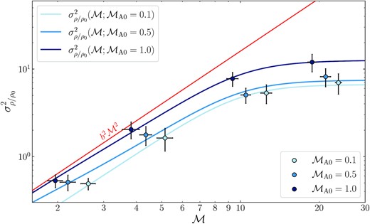
Two-shock model (equation 32) for the density variance, |$\sigma ^2_{\rho /\rho _0}$|⁠, as a function of |$\mathcal {M}$|⁠, for each set of |$\operatorname{\mathcal {M}_{\text{A0}}}$| simulations. Blue points are numerical data from the 12 simulations (Table 1), averaged over a time interval of |$5\, T$|⁠. The red line indicates the hydrodynamical limit for the density variance, |$b^2\mathcal {M}^2$|⁠. We find that the variance grows from low-|$\mathcal {M}$| to |$\mathcal {M}\approx 4$| in a hydrodynamical fashion, but then saturates as the small-scale density fluctuations (associated with high-|$\mathcal {M}$| values) are suppressed by the strong mean magnetic field. We plot our model, equation (32), on each |$\operatorname{\mathcal {M}_{\text{A0}}}$| data set, shown with the solid lines. We find good agreement between the data and our models, which suggests there is an upper bound for |$\sigma ^2_{\rho /\rho _0}$| in this highly magnetized, anisotropic turbulent regime. We discuss the implications for this result in Section 7.

Open in new tab Download slide

Our results establish the following picture of the density field in this regime: at low-|$\mathcal {M}$|⁠, hydrodynamical, parallel to |${B}_0$|⁠, fluctuations are large scale, occupying a significant fraction of the fluid volume with a relatively large volume-filling fraction. The type I shocks dominate the parallel fluctuation contribution to the volume-weighted variance of the density field. However, as |$\mathcal {M}$| increases, the small-scale fluctuations grow in the field, and the type I shocks shrink in size with their shock width |${\sim} \mathcal {M}^{-2}$|⁠, and thus the parallel fluctuations begin to occupy only very small fractions of the fluid volume, decreasing the contribution from type I shocks to the variance. When |$\mathcal {M}\gg 1$|⁠, the total volume-weighted variance becomes by type II shocks, which are highly magnetized and do not support small-scale fluctuations. This flattens |$\sigma _{\rho /\rho _0}^2(\mathcal {M})$| out, because the small-scale fluctuations that are added to the field with increasing |$\mathcal {M}$| are suppressed. Eventually this leads to an upper bound on |$\sigma _{\rho /\rho _0}^2$|⁠, as the type II shock density contrasts dominate the total variance.

6.1 Limiting behaviour of the model

Let us now consider the limiting behaviour of the density variance in our model. The density variance is summarized as

$$\begin{eqnarray*} \sigma ^2_{\rho /\rho _0} = f_{\parallel } \sigma ^2_{\rho /\rho _0\parallel } + (1 - f_{\parallel })\sigma ^2_{\rho /\rho _0\perp }. \end{eqnarray*}$$

(48)

In the high-|$\mathcal {M}$| limit we have

$$\begin{eqnarray*} \lim _{\mathcal {M}\rightarrow \infty } \sigma ^2_{\rho /\rho _0} = f_0 b^2\mathcal {M}_{\rm c}^2 + \frac{1}{2}\left(\sqrt{1 + 8\mathcal {M}^{2}_{\text{A0}}}-1\right), \end{eqnarray*}$$

(49)

which, like the density contrast caused by type II shocks shown in Section 3.2.2, is asymptotic to a limit fixed by the magnetic field and turbulent parameters. Ours is the first model to predict such a bound for the total density fluctuations, which is set by the strength of the mean magnetic field, the type of driving, and the volume-filling fraction of subsonic fluctuations travelling along |${B}_0$|⁠. This tells us that even in the high-|$\mathcal {M}$| limit the turbulent driving parameter influences the spread of the PDF, frozen into the variance at high-|$\mathcal {M}$|⁠. Interestingly, the limiting behaviour is independent of |$\mathcal {M}$|⁠, as the effect of increasingly sharp density contrasts (⁠|$\mathcal {M}^2$|⁠) of supersonic hydrodynamical shocks is cancelled out by the reduced volume-filling factor of the parallel fluctuations.

The next limit of interest is the low-|$\operatorname{\mathcal {M}_{\text{A0}}}$| limit,

$$\begin{eqnarray*} \lim _{\operatorname{\mathcal {M}_{\text{A0}}}\rightarrow 0} \sigma ^2_{\rho /\rho _0} = f_{\parallel } b^2 \mathcal {M}^2. \end{eqnarray*}$$

(50)

Thus, the parallel component of the variance is retained in this limit. We can interpret this as hydrodynamical fluctuations are able to survive along the magnetic field but are confined in a small volume, |$f_{\parallel }\mathcal {V}$|⁠, and hence are reduced by the volume-filling fraction, f_∥. This value will be significantly less than 1 for |$\mathcal {M}\gg 10$|⁠, as measured in Section 5.2. This is a key distinguishing feature from any of the isotropic magnetized models presented in equation (13) (Molina et al. 2012). Both of these models result in |$\sigma ^2_{\rho /\rho _0} = 0$| in this limit.

Finally, in the high-|$\operatorname{\mathcal {M}_{\text{A0}}}$| limit, as the turbulence transitions from magnetized to hydrodynamic,

$$\begin{eqnarray*} \lim _{\operatorname{\mathcal {M}_{\text{A0}}}\rightarrow \infty } \sigma ^2_{\rho /\rho _0} = f_{\parallel } b^2\mathcal {M}^2 + (1 - f_{\parallel }) b^2\mathcal {M}^2 = b^2\mathcal {M}^2, \end{eqnarray*}$$

(51)

which is the well-known, isotropic, hydrodynamic |$\mathcal {M}\!-\!\sigma ^2_{\rho /\rho _0}$| relation.

7 DISCUSSION

7.1 Implications for density fluctuations observed in the ISM

We motivated in Section 1 that there have been a number of ISM observations (Li & Henning 2011; Li et al. 2013; Soler et al. 2013, 2017; Cox et al. 2016; Federrath 2016b; Malinen et al. 2016; Planck Collaboration XXXIV 2016a; Planck Collaboration XXXV 2016b; Tritsis & Tassis 2016; Tritsis et al. 2018; Heyer et al. 2020; Pillai et al. 2020) and simulations (Soler & Hennebelle 2017; Tritsis et al. 2018; Beattie & Federrath 2020; Körtgen & Soler 2020; Seifried et al. 2020; Barreto-Mota et al. 2021) that show bimodally distributed density structures with respect to the magnetic field.

For example, recent polarimetric observations of nearby MCs reveal that the alignment of filamentary structures in gas column density derived from Herschel submillimetre observations change with the density: high-density structures (⁠|$N_{\rm H_2} \propto 10^{23}\, \text{cm}^{-2}$|⁠, where |$N_{\rm H_2}$| is the number density of the molecular gas column density) tend to be oriented perpendicularly to, and low-density (⁠|$N_{\rm H_2} \propto 10^{22}\, \text{cm}^{-2}$|⁠) structures parallel to, the mean magnetic field (Planck Collaboration XXXIV 2016a; Soler et al. 2017; Tritsis et al. 2018; Heyer et al. 2020; Pillai et al. 2020). Through the analysis of numerical MHD turbulence simulations we have identified some of the physics that causes the bimodal alignment of gas density structures during this density transition. To summarize, the alignment in simulations like ours comes about through an interplay between the divergence (compressibility) and the strain (most likely associated with vortex creation; such as those visualized in Fig. 4) in the flow. This has been found in multiple studies of highly magnetized, compressible plasmas, including those simulations presented in Fig. 6 (Soler & Hennebelle 2017; Beattie & Federrath 2020; Körtgen & Soler 2020; Seifried et al. 2020). A different model is developed in Xu, Ji & Lazarian (2019). They use the Goldreich & Sridhar (1995) anisotropy theory to model the extent of low-density filaments in the warm, diffuse and subsonic ISM. This model is most likely not applicable for the highly compressible flows in the supersonic, cool, and dense MCs, which need not conform to the incompressible Goldreich & Sridhar (1995) theory. The transition occurs with or without the presence of self-gravity, and hence seems to be a MHD phenomenon (however, self-gravitating MHD simulations are shown to enhance the density structures that are perpendicular to |${B}_0$|⁠; e.g. Soler & Hennebelle 2017; Gómez, Vázquez-Semadeni & Zamora-Avilés 2018; Barreto-Mota et al. 2021).

Our two-shock model suggests a simple explanation for this density transition described above, irrespective of the physical processes that create the aligned structures, which is beyond the scope of this study. The shock-jump conditions predict that perpendicularly oriented hydrodynamical shocks formed from material flowing along the magnetic field are at least an order of magnitude larger in density contrast compared to parallel-oriented fast magnetosonic shocks, formed through shuffling magnetic field lines. We show this qualitatively in Fig. 6, with the density contrasts produced by the shocks visualized in the two bottom panels. Hence, we suggest that the observed transition in the density arises from observing these two distinct types of MHD modes.

A further transition is also now reported at even higher column densities, within the filaments (<0.1 pc) themselves (Pillai et al. 2020). Inside of the filaments gravity-induced accretion gas flows entrain the magnetic field, realigning it with the gas flow. This creates parallel aligned gas channels that accrete on to, for example, hubs between high-density perpendicular-oriented filaments (Gómez et al. 2018; Busquet 2020; Pillai et al. 2020).

Pioneering work from Soler & Hennebelle (2017) characterized the bimodality of the first transition in terms of the angle, ϕ, between ∇ρ and |${B}$|⁠. They showed that cos ϕ = ±1 and cos ϕ = 0 constitute equilibrium points that an ideal MHD system tends towards. In our work, we demonstrated that the physical realization of this insight corresponds to hydrodynamical shocks that form along |${B}_0$| (cos ϕ = 0) and fast magnetosonic shocks that form perpendicular to |${B}_0$| (cos ϕ = ±1). From the perspective of linear MHD wave theory, these are the only two waves that are able to compress the density and form the |$\nabla \cdot \mathbf {v} \lt 0$| structures in the flow. We hypothesize that at least for some sub-Alfvénic, supersonic MCs it is these compressible MHD modes that form the overdense seeds and allow a local region to become Jeans unstable and collapse under gravity.

7.2 Implications for star formation theory

Bottom-up star formation theories treat MCs as the fundamental building blocks that determine galactic star formation rates, and are parametrized by |$\sigma _{\rho /\rho _0}^2$|⁠, as discussed in Section 1 (Krumholz & McKee 2005; Hennebelle et al. 2011; Padoan & Nordlund 2011; Federrath & Klessen 2012, 2013; Federrath & Banerjee 2015; Mocz et al. 2017; Burkhart 2018; Hennebelle & Inutsuka 2019; Lee & Hennebelle 2019; Lee et al. 2020). Turbulence regulation, in the context of these models, is cast as a battle between density variance, |$\sigma _{\rho /\rho _0}^2$|⁠, and (ρ/ρ₀)_crit, the critical density at which the cloud becomes Jeans unstable and collapses (Federrath 2018). The magnetic field plays a role in these models by reducing the total density variance (as shown in equation 13), and by introducing additional support through magnetic pressure in the critical density, preventing collapse (Krumholz & McKee 2005; Federrath & Klessen 2012, 2013). However, all of these models treat the magnetic field only as an isotropic contribution via the magnetic pressure. The effects of magnetic tension or the anisotropic effects introduced by a strong guide field are not included in the current theories of star formation. Here we show that the magnetic field, specifically, a sub-Alfvénic mean field, which encodes tension into the theory, acts preferentially to suppress small-scale density fluctuations (and hence turbulent fragmentation), preventing |$\sigma _{\rho /\rho _0}^2$| from growing beyond a specific limit set by the strength of the field, shown in equation (49) and in the ln ρ/ρ₀–PDFs in Fig. 2. This is an extra form of suppression that B₀ has on the star formation rate.

A complete theory for anisotropic star formation would take into account that fluctuations perpendicular to the magnetic field are suppressed significantly, whereas along the field they are not. As such, the theory would predict that star formation may become bimodal with respect to the direction of the large-scale coherent |${B}$|-field. There are some observational signatures that this may be the case with the star formation rate of some MCs seeming to depend upon the large-scale orientation of the magnetic field (Law, Li & Leung 2019; Law et al. 2020).

In this study, we describe a model for the variance applicable to these types of MCs, but to properly predict the star formation rate in a strongly magnetized environment one also must create an anisotropic model for (ρ/ρ₀)_crit, which contains both information about the scale in which the turbulence transitions from supersonic to subsonic in rms velocities, i.e. the sonic scale (Federrath & Klessen 2012; Federrath et al. 2021), and the Jeans scale. The morphology of the sonic scale in the presence of a strong magnetic field is unknown, but one can speculate that it most likely will become stretched along the field lines, changing the nature of the critical density, and how cloud collapse happens in this regime. What we emphasize here is that there is much work to do in this supersonic, anisotropic, highly magnetized regime, much of which we intend to pursue in future studies.

8 SUMMARY AND KEY FINDINGS

In this study, we explore the density variance, |$\sigma _{\rho /\rho _0}^2$|⁠, of highly magnetized, anisotropic, supersonic turbulence across and along the mean magnetic field, |${B}_0$|⁠. In Section 2, we discuss the derivation of the |$\sigma _{\rho /\rho _0}^2 \!-\! \mathcal {M}$| relation and highlight the fundamental connection between shock-jump conditions for the density field and |$\sigma _{\rho /\rho _0}^2$|⁠. In Section 3, we describe in detail how we define the geometry of shocks, and finally, we derive our two-shock model for |$\sigma _{\rho /\rho _0}^2$|⁠. In Section 4, we discuss the set-up and data processing for the 12 supersonic (⁠|$\mathcal {M}\gt 1$|⁠; where |$\mathcal {M}$| is the sonic Mach number), trans-/sub-Alfvénic (⁠|$\operatorname{\mathcal {M}_{\text{A0}}}\le 1$|⁠; where |$\operatorname{\mathcal {M}_{\text{A0}}}$| is the mean-field Alfvénic Mach number) MHD simulations. We show examples of the 2D density slices and the full 3D density fields in Figs 3 and 4, respectively. In Section 5, we fit our two-shock density model to the variance data, and in Section 6, we discuss the results from the fit. We summarize the fitting process in the following steps.

We derive a model for the density variance that takes the general form |$\sigma _{\rho /\rho _0}^2 = f_{\parallel }\sigma _{\rho /\rho _0\parallel }^2 + f_{\perp }\sigma _{\rho /\rho _0\perp }^2$|⁠, where |$\sigma _{\rho /\rho _0\parallel }^2$| comes from type I shocks and |$\sigma _{\rho /\rho _0\perp }^2$| comes from type II shocks.
The entire volume of the turbulence must contribute to the total variance, hence we assume that f_∥ = 1 − f_⊥. This defines a single-parameter model |$\sigma _{\rho /\rho _0}^2 = f_{\parallel }\sigma _{\rho /\rho _0\parallel }^2 + (1-f_{\parallel })\sigma _{\rho /\rho _0\perp }^2$|⁠.
We propose a phenomenological model for f_∥, |$f_{\parallel } = f_0\left[1 + \left(\frac{\mathcal {M}}{\mathcal {M}_{\rm c}}\right)^4 \right]^{-1/2}$|⁠, based on the shock thickness of type I shocks.
We use numerical simulations parametrized by |$(\mathcal {M},\mathcal {M}_{\rm A0})$| to directly measure |$\sigma _{\rho /\rho _0}^2$|⁠, and calculate |$\sigma _{\rho /\rho _0\parallel }^2$| and |$\sigma _{\rho /\rho _0\perp }^2$|⁠.
Using the numerical data we fit for the two parameters in the f_∥ model, f₀, which is associated with the volume-filling fraction of the parallel fluctuations in the subsonic limit, and |$\mathcal {M}_{\rm c}$| is the |$\mathcal {M}$| when the supersonic flow is significantly saturated with shocks.

Finally, in Section 7, we discuss the implications for ISM structure and magnetized star formation theory. We summarize the key results below.

We derive a model for the density variance, |$\sigma ^2_{\rho /\rho _0}$|⁠, in a sub-Alfvénic, supersonic, anisotropic flow regime, where a strong mean magnetic field, |${B}_0$|⁠, creates dynamically different fluctuations parallel and perpendicular to field, characterized by equation (32). To do this, we generalize the shock variance relations from Padoan & Nordlund (2011) and Molina et al. (2012), discussed in Section 3, partitioning the total volume into two subvolumes that contain hydrodynamical shocks moving along (parallel to) the magnetic field, and fast magnetosonic shocks moving across (perpendicular to) the field, with details of the orientation and compression mechanism shown in Fig. 1.
Our density variance model relies upon the volume-filling fraction, f_∥ – a measure of how much relative volume the parallel fluctuations occupy along |${B}_0$|⁠. We propose a phenomenological model for f_∥, equation (46), using the shock width described in Padoan & Nordlund (2011), discussed in detail in Section 5.1. Using the numerical simulations, we fit our model, with fit parameters listed in Table 2, and illustrated in Fig. 5. By assuming that the parallel and perpendicular fluctuations must occupy the whole volume, we find the parallel fluctuations dominate the volume budget in low-|$\mathcal {M}$| flows, whilst the perpendicular fluctuations dominate in high-|$\mathcal {M}$| flows, consistent with the compressible structures visualized in Figs 3 and 6.
Our new model predicts a finite value of |$\sigma ^2_{\rho /\rho _0}$| in the high-|$\mathcal {M}$| limit, shown in equation (49), which is set by the strength of |${B}_0$|⁠. This is because a strong |${B}_0$| field acts preferentially to suppress the small-scale fluctuations introduced in high-|$\mathcal {M}$| flows. The new model also predicts a finite value of |$\sigma ^2_{\rho /\rho _0}$| as B₀ → ∞, as shown in equation (50), corresponding to density fluctuations that can persist along |${B}_0$|⁠. In the hydrodynamical limit, as shown in equation (51), our model reduces to the well-known relation, |$\sigma ^2_{\rho /\rho _0} = b^2\mathcal {M}^2$|⁠, where b is the turbulent driving parameter. We demonstrate that our variance model provides a good fit to the simulation data in Fig. 7.
In Section 7, we discuss how the two different MHD shocks that we use in our model may explain the density transition observed in some nearby MCs. This because the fast magnetosonic shocks, which create density fluctuations parallel to the magnetic field, have density contrasts at least an order of magnitude less than the hydrodynamical shocks, which cause density fluctuations perpendicular to the magnetic field. We also highlight how a strong |${B}_0$| may additionally suppress star formation by limiting the small-scale density fluctuations, and hence turbulent fragmentation in MCs with |$\mathcal {M}\gtrsim 4$|⁠.

ACKNOWLEDGEMENTS

We thank the anonymous reviewer for their detailed review, which increased the clarity and presentation of the study. JRB thanks Shyam Menon for the many productive discussions and acknowledges financial support from the Australian National University, via the Deakin PhD and Dean’s Higher Degree Research (theoretical physics) Scholarships, the Research School of Astronomy and Astrophysics, via the Joan Duffield Research Scholarship, and the Australian Government via the Australian Government Research Training Program Fee-Offset Scholarship. PM acknowledges support for this work provided by NASA through Einstein Postdoctoral Fellowship grant number PF7-180164 awarded by the Chandra X-ray Center, which is operated by the Smithsonian Astrophysical Observatory for NASA under contract NAS8-03060. CF acknowledges funding provided by the Australian Research Council (Discovery Project DP170100603 and Future Fellowship FT180100495), and the Australia–Germany Joint Research Cooperation Scheme (UA-DAAD). RSK acknowledges financial support from the German Research Foundation (DFG) via the Collaborative Research Center (SFB 881, Project-ID 138713538) ‘The Milky Way System’ (subprojects A1, B1, B2, and B8). RSK also thanks for funding from the Heidelberg Cluster of Excellence STRUCTURES in the framework of Germany’s Excellence Strategy (grant EXC-2181/1 - 390900948) and for funding from the European Research Council via the ERC Synergy Grant ECOGAL (grant 855130). We further acknowledge high-performance computing resources provided by the Australian National Computational Infrastructure (grant ek9) in the framework of the National Computational Merit Allocation Scheme and the ANU Merit Allocation Scheme, and by the Leibniz-Rechenzentrum and the Gauss Centre for Supercomputing (grants pr32lo, pr48pi, pr74nu). The simulation software flash was in part developed by the DOE-supported Flash Centre for Computational Science at the University of Chicago.

Data analysis and visualization software used in this study: c++ (Stroustrup 2013), numpy (Oliphant 2006; Harris et al. 2020), matplotlib (Hunter 2007), cython (Behnel et al. 2011), visit (Childs et al. 2012), scipy (Virtanen et al. 2020), and scikit-image (van der Walt et al. 2014). The colour maps used in Figs 3 and 6 are sourced from the python package cmasher (van der Velden 2020).

DATA AVAILABILITY

The data underlying this paper will be shared on reasonable request to the corresponding author.

Footnotes

1

Not all MCs are sub-Alfvénic in nature. See, for example, Lunttila et al. (2008) for quite convincing results that clouds observed in Troland & Crutcher (2008) are super-Alfvénic based on the magnetic and column density field correlations. The clouds we list as sub-Alfvénic are not part of the survey reported in Troland & Crutcher (2008).

2

For a lognormally distributed variable, ρ/ρ₀, the variance of the log-variable obeys |$\sigma _{\ln \rho /\rho _0}^2 = \ln (1 + \sigma ^2_{\rho /\rho _0})$| and is the value that is commonly reported in the literature. Throughout this study we however consider |$\sigma ^2_{\rho /\rho _0}$|⁠, without making any assumptions of the underlying distribution.

3

By expressing the variance as we have below we are assuming that the density fluctuations are symmetric around the magnetic field. This was shown explicitly through the elliptic symmetry with respect to the magnetic field of the 2D density power spectra in fig. 2 of Beattie & Federrath (2020) and 2D structure functions in Hu, Lazarian & Bialy (2020).

4

This is a justified assumption because the statistically averaged elliptic power spectra in fig. 2 of Beattie & Federrath (2020) do not show any rotations in the k_⊥–k_∥ plane, i.e. the principal axes of the ellipses fitted to the power spectra are aligned with the k_⊥–k_∥ coordinate axis, where k_⊥ corresponds to wavenumbers perpendicular to |${B}_0$| and k_∥ for parallel wavenumbers. This means that the density fluctuations along and across the mean field are statistically independent from each other, and hence |$2\sigma _{\rho /\rho _0 \parallel }\sigma _{\rho /\rho _0 \perp } \approx 0$|⁠.

5

We consider the transformation |$\operatorname{d}\!{\mathcal {V}}= |\frac{\operatorname{d}\!{\mathcal {V}}}{\operatorname{d}\!{(}\rho _1/\rho _0)} |\operatorname{d}\!{(}\rho _1/\rho _0)$| to simplify the treatment of the limits in equation (21).

6

Note that we integrate ρ₁/ρ₀ from 1, i.e. when the pre- and post-shock densities are the same, up to an arbitrarily large density contrast, ρ/ρ₀. This is the range of density contrasts where a shock is well defined.

7

We use the same definition as equation (6), but using the mean magnetic field instead of the total field, hence, |$\operatorname{\mathcal {M}_{\text{A0}}}= \sigma _V / V_{\rm A0}$|⁠, where |$V_{\rm A0} = B_0 / \sqrt{4\pi \rho _0}$|⁠.

8

This follows from |$\sigma ^2_{\rho /\rho _0} = f_{\parallel }\sigma ^2_{\rho /\rho _0\parallel } + f_{\perp }\sigma ^2_{\rho /\rho _0\perp } = f_{\parallel }\sigma ^2_{\rho /\rho _0\parallel } + (1 - f_{\parallel })\sigma ^2_{\rho /\rho _0\perp }$| and then solving for f_∥.

REFERENCES

Abe

D.

,

Inoue

T.

,

Inutsuka

S.-I.

,

Matsumoto

T.

,

2020

,

preprint (arXiv:2012.02205)

Barreto-Mota

L.

,

de Gouveia Dal Pino

E. M.

,

Burkhart

B.

,

Melioli

C.

,

Santos-Lima

R.

,

Kadowaki

L. H. S.

,

2021

,

MNRAS

,

503

,

5425

Beattie

J. R.

,

Federrath

C.

,

2020

,

MNRAS

,

492

,

668

10.1093/mnras/stz3377

Crossref

Beattie

J. R.

,

Federrath

C.

,

Klessen

R. S.

,

2019a

,

MNRAS

,

487

,

2070

10.1093/mnras/stz1416

Crossref

Beattie

J. R.

,

Federrath

C.

,

Klessen

R. S.

,

Schneider

N.

,

2019b

,

MNRAS

,

488

,

2493

10.1093/mnras/stz1853

Crossref

Beattie

J. R.

,

Federrath

C.

,

Seta

A.

,

2020

,

MNRAS

,

498

,

1593

10.1093/mnras/staa2257

Crossref

Behnel

S.

,

Bradshaw

R.

,

Citro

C.

,

Dalcin

L.

,

Seljebotn

D. S.

,

Smith

K.

,

2011

,

Comput. Sci. Eng.

,

13

,

31

Bialy

S.

,

Burkhart

B.

,

2020

,

ApJ

,

894

,

L2

10.3847/2041-8213/ab8a32

Crossref

Boldyrev

S.

,

2006

,

Phys. Rev. Lett.

,

96

,

115002

10.1103/PhysRevLett.96.115002

Crossref

Bouchut

F.

,

Klingenberg

C.

,

Waagan

K.

,

2010

,

Numer. Math.

,

115

,

647

10.1007/s00211-010-0289-4

Crossref

Burgers

J.

,

1948

,

Adv. Appl. Mech.

,

1

,

171

http://dx.doi.org/10.1016/S0065-2156(08)70100-5

Burkhart

B.

,

2018

,

ApJ

,

863

,

118

10.3847/1538-4357/aad002

Crossref

Burkhart

B.

,

Lazarian

A.

,

2012

,

ApJ

,

755

,

L19

10.1088/2041-8205/755/1/l19

Crossref

Burkhart

B.

,

Falceta-Gonçalves

D.

,

Kowal

G.

,

Lazarian

A.

,

2009

,

ApJ

,

693

,

250

10.1088/0004-637x/693/1/250

Crossref

Burkhart

B.

,

Lazarian

A.

,

Leão

I. C.

,

de Medeiros

J. R.

,

Esquivel

A.

,

2014

,

ApJ

,

790

,

130

10.1088/0004-637X/790/2/130

Crossref

Busquet

G.

,

2020

,

Nat. Astron.

,

4

,

1126

10.1038/s41550-020-1180-6

Crossref

Childs

H.

et al. ,

2012

, in

Wes Bethel

E.

,

Childs

H.

,

Hansen

C.

, eds,

High Performance Visualization–Enabling Extreme-Scale Scientific Insight

.

CRC Press/Taylor & Francis Group

,

Boca Raton, FL

, p.

357

Google Scholar

Google Preview

OpenURL Placeholder Text

WorldCat

Cho

J.

,

Lazarian

A.

,

Vishniac

E. T.

,

2002

,

ApJ

,

564

,

291

10.1086/324186

Crossref

Cox

N. L. J.

et al. ,

2016

,

A&A

,

590

,

A110

10.1051/0004-6361/201527068

Crossref

Dubey

A.

et al. ,

2008

, in

Pogorelov

N. V.

,

Audit

E.

,

Zank

G. P.

, eds,

ASP Conf. Ser. Vol. 385, Numerical Modeling of Space Plasma Flows

.

Astron. Soc. Pac

,

San Francisco

, p.

145

Google Scholar

Google Preview

OpenURL Placeholder Text

WorldCat

Federrath

C.

,

2013

,

MNRAS

,

436

,

1245

10.1093/mnras/stt1644

Crossref

Federrath

C.

,

2016a

,

J. Plasma Phys.

,

82

,

535820601

10.1017/S0022377816001069

Crossref

Federrath

C.

,

2016b

,

MNRAS

,

457

,

375

10.1093/mnras/stv2880

Crossref

Federrath

C.

,

2018

,

Phys. Today

,

71

,

38

10.1063/PT.3.3947

Crossref

Federrath

C.

,

Banerjee

S.

,

2015

,

MNRAS

,

448

,

3297

10.1093/mnras/stv180

Crossref

Federrath

C.

,

Klessen

R. S.

,

2012

,

ApJ

,

761

,

156

10.1088/0004-637X/761/2/156

Crossref

Federrath

C.

,

Klessen

R. S.

,

2013

,

ApJ

,

763

,

51

10.1088/0004-637X/763/1/51

Crossref

Federrath

C.

,

Klessen

R. S.

,

Schmidt

W.

,

2008

,

ApJ

,

688

,

L79

10.1086/595280

Crossref

Federrath

C.

,

Klessen

R. S.

,

Schmidt

W.

,

2009

,

ApJ

,

692

,

364

10.1086/595280

Crossref

Federrath

C.

,

Roman-Duval

J.

,

Klessen

R. S.

,

Schmidt

W.

,

Mac Low

M.-M.

,

2010

,

A&A

,

512

,

A81

10.1051/0004-6361/200912437

Crossref

Federrath

C.

et al. ,

2016

,

ApJ

,

832

,

143

10.3847/0004-637X/832/2/143

Crossref

Federrath

C.

,

Klessen

R. S.

,

Iapichino

L.

,

Beattie

J. R.

,

2021

,

Nat. Astron.

,

5

,

365

–

371

.

Fryxell

B.

et al. ,

2000

,

ApJS

,

131

,

273

10.1086/317361

Crossref

Ginsburg

A.

,

Federrath

C.

,

Darling

J.

,

2013

,

ApJ

,

779

,

50

10.1088/0004-637X/779/1/50

Crossref

Goldreich

P.

,

Sridhar

S.

,

1995

,

ApJ

,

438

,

763

10.1086/175121

Crossref

Gómez

G. C.

,

Vázquez-Semadeni

E.

,

Zamora-Avilés

M.

,

2018

,

MNRAS

,

480

,

2939

10.1093/mnras/sty2018

Crossref

Harris

C. R.

et al. ,

2020

,

Nature

,

585

,

357

10.1038/s41586-020-2649-2

Crossref

Hennebelle

P.

,

Chabrier

G.

,

2008

,

ApJ

,

684

,

395

10.1086/589916

Crossref

Hennebelle

P.

,

Chabrier

G.

,

2009

,

ApJ

,

702

,

1428

10.1088/0004-637X/702/2/1428

Crossref

Hennebelle

P.

,

Inutsuka

S.-i.

,

2019

,

Frontiers Astron. Space Sci.

,

6

,

5

10.3389/fspas.2019.00005

Crossref

Hennebelle

P.

,

Commerçon

B.

,

Joos

M.

,

Klessen

R. S.

,

Krumholz

M.

,

Tan

J. C.

,

Teyssier

R.

,

2011

,

A&A

,

528

,

A72

10.1051/0004-6361/201016052

Crossref

Heyer

M.

,

Soler

J. D.

,

Burkhart

B.

,

2020

,

MNRAS

,

496

,

4546

10.1093/mnras/staa1760

Crossref

Hopkins

P. F.

,

2013a

,

MNRAS

,

430

,

1653

10.1093/mnras/sts704

Crossref

Hopkins

P. F.

,

2013b

,

MNRAS

,

430

,

1880

10.1093/mnras/stt010

Crossref

Hu

Y.

et al. ,

2019

,

Nat. Astron.

,

3

,

776

10.1038/s41550-019-0769-0

Crossref

Hu

Y.

,

Lazarian

A.

,

Bialy

S.

,

2020

,

ApJ

,

905

,

129

10.3847/1538-4357/abc3c6

Crossref

Hunter

J. D.

,

2007

,

Comput. Sci. Eng.

,

9

,

90

10.1109/MCSE.2007.55

Crossref

Kainulainen

J.

,

Federrath

C.

,

Henning

T.

,

2014

,

Science

,

344

,

183

10.1126/science.1248724

Crossref

Kim

J.

,

Ryu

D.

,

2005

,

ApJ

,

630

,

L45

10.1086/491600

Crossref

Klessen

R. S.

,

Glover

S. C. O.

,

2016

, in

Revaz

Y.

,

Jablonka

P.

,

Teyssier

R.

,

Mayer

L.

, eds,

Saas-Fee Advanced Course Vol. 43, Star Formation in Galaxy Evolution: Connecting Numerical Models to Reality

.

Springer-Verlag

,

Berlin

, p.

85

10.1007/978-3-662-47890-5_2

Crossref

Klessen

R. S.

,

Heitsch

F.

,

Mac Low

M.-M.

,

2000

,

ApJ

,

535

,

887

10.1086/308891

Crossref

Konstandin

L.

,

Federrath

C.

,

Klessen

R. S.

,

Schmidt

W.

,

2012a

,

J. Fluid Mech.

,

692

,

183

10.1017/jfm.2011.503

Crossref

Konstandin

L.

,

Girichidis

P.

,

Federrath

C.

,

Klessen

R. S.

,

2012b

,

ApJ

,

761

,

149

10.1088/0004-637X/761/2/149

Crossref

Konstandin

L.

,

Schmidt

W.

,

Girichidis

P.

,

Peters

T.

,

Shetty

R.

,

Klessen

R. S.

,

2016

,

MNRAS

,

460

,

4483

10.1093/mnras/stw1313

Crossref

Körtgen

B.

,

Soler

J. D.

,

2020

,

MNRAS

,

499

,

4785

10.1093/mnras/staa3078

Crossref

Krumholz

M. R.

,

Federrath

C.

,

2019

,

Frontiers Astron. Space Sci.

,

6

,

7

10.3389/fspas.2019.00007

Crossref

Krumholz

M. R.

,

McKee

C. F.

,

2005

,

ApJ

,

630

,

250

10.1086/431734

Crossref

Landau

L. D.

,

Lifshitz

E. M.

,

1959

,

Course of Theoretical Physics Vol. 6, Fluid Mechanics

.

Pergamon Press

,

Oxford

Google Scholar

Google Preview

OpenURL Placeholder Text

WorldCat

Law

C. Y.

,

Li

H. B.

,

Leung

P. K.

,

2019

,

MNRAS

,

484

,

3604

10.1093/mnras/stz244

Crossref

Law

C. Y.

,

Li

H. B.

,

Cao

Z.

,

Ng

C. Y.

,

2020

,

MNRAS

,

498

,

850

10.1093/mnras/staa2466

Crossref

Lee

Y.-N.

,

Hennebelle

P.

,

2019

,

A&A

,

622

,

A125

10.1051/0004-6361/201834428

Crossref

Lee

Y.-N.

,

Offner

S. S. R.

,

Hennebelle

P.

,

André

P.

,

Zinnecker

H.

,

Ballesteros-Paredes

J.

,

Inutsuka

S.-I.

,

Kruijssen

J. M. D.

,

2020

,

Space Sci. Rev.

,

216

,

70

10.1007/s11214-020-00699-2

Crossref

Lehmann

A.

,

Federrath

C.

,

Wardle

M.

,

2016

,

MNRAS

,

463

,

1026

10.1093/mnras/stw2015

Crossref

Li

H.-B.

,

Henning

T.

,

2011

,

Nature

,

479

,

499

10.1038/nature10551

Crossref

Li

H.-b.

,

Fang

M.

,

Henning

T.

,

Kainulainen

J.

,

2013

,

MNRAS

,

436

,

3707

10.1093/mnras/stt1849

Crossref

Lunttila

T.

,

Padoan

P.

,

Juvela

M.

,

Nordlund

Å.

,

2008

,

ApJ

,

686

,

L91

10.1086/593032

Crossref

Mac Low

M. M.

,

Klessen

R. S.

,

2004

,

Rev. Mod. Phys.

,

76

,

125

10.1103/RevModPhys.76.125

Crossref

Malinen

J.

et al. ,

2016

,

MNRAS

,

460

,

1934

10.1093/mnras/stw1061

Crossref

Matthaeus

W. H.

,

Pouquet

A.

,

Mininni

P. D.

,

Dmitruk

P.

,

Breech

B.

,

2008

,

Phys. Rev. Lett.

,

100

,

085003

10.1103/PhysRevLett.100.085003

Crossref

Menon

S. H.

,

Federrath

C.

,

Klaassen

P.

,

Kuiper

R.

,

Reiter

M.

,

2021

,

MNRAS

,

500

,

1721

10.1093/mnras/staa3271

Crossref

Mocz

P.

,

Burkhart

B.

,

2018

,

MNRAS

,

480

,

3916

10.1093/mnras/sty1976

Crossref

Mocz

P.

,

Burkhart

B.

,

2019

,

ApJ

,

884

,

L35

10.3847/2041-8213/ab48f6

Crossref

Mocz

P.

,

Burkhart

B.

,

Hernquist

L.

,

McKee

C. F.

,

Springel

V.

,

2017

,

ApJ

,

838

,

40

10.3847/1538-4357/aa6475

Crossref

Mohapatra

R.

,

Federrath

C.

,

Sharma

P.

,

2020

,

MNRAS

,

493

,

5838

10.1093/mnras/staa711

Crossref

Mohapatra

R.

,

Federrath

C.

,

Sharma

P.

,

2021

,

MNRAS

,

500

,

5072

Molina

F. Z.

,

Glover

S. C. O.

,

Federrath

C.

,

Klessen

R. S.

,

2012

,

MNRAS

,

423

,

2680

10.1111/j.1365-2966.2012.21075.x

Crossref

Nolan

C. A.

,

Federrath

C.

,

Sutherland

R. S.

,

2015

,

MNRAS

,

451

,

1380

10.1093/mnras/stv1030

Crossref

Oliphant

T.

,

2006

,

NumPy: A Guide to NumPy

.

Trelgol Publishing

,

USA

(http://www.numpy.org/)

Google Scholar

Google Preview

OpenURL Placeholder Text

WorldCat

Orkisz

J. H.

et al. ,

2017

,

A&A

,

599

,

A99

10.1051/0004-6361/201629220

Crossref

Padoan

P.

,

Nordlund

Å.

,

2002

,

ApJ

,

576

,

870

10.1086/341790

Crossref

Padoan

P.

,

Nordlund

Å.

,

2011

,

ApJ

,

730

,

40

10.1088/0004-637X/730/1/40

Crossref

Padoan

P.

,

Nordlund

P.

,

Jones

B. J. T.

,

1997

,

Commmun. Konkoly Obser. Hungary

,

100

,

341

Palmeirim

P.

et al. ,

2013

,

A&A

,

550

,

A38

10.1051/0004-6361/201220500

Crossref

Park

J.

,

Ryu

D.

,

2019

,

ApJ

,

875

,

2

10.3847/1538-4357/ab0d7e

Crossref

Passot

T.

,

Vázquez-Semadeni

E.

,

1998

,

Phys. Rev. E

,

58

,

4501

10.1103/PhysRevE.58.4501

Crossref

Pillai

T.

,

Kauffmann

J.

,

Tan

J. C.

,

Goldsmith

P. F.

,

Carey

S. J.

,

Menten

K. M.

,

2015

,

ApJ

,

799

,

74

10.1088/0004-637x/799/1/74

Crossref

Pillai

T. G. S.

et al. ,

2020

,

Nat. Astron.

,

4

,

1195

10.1038/s41550-020-1172-6

Crossref

Planck Collaboration XXXIV

,

2016a

,

A&A

,

586

,

A137

10.1051/0004-6361/201525616

Crossref

Planck Collaboration XXXV

,

2016b

,

A&A

,

586

,

A138

10.1051/0004-6361/201525896

Crossref

Price

D. J.

,

Federrath

C.

,

2010

,

MNRAS

,

406

,

1659

10.1111/j.1365-2966.2010.16810.x

Crossref

Price

D. J.

,

Federrath

C.

,

Brunt

C. M.

,

2011

,

ApJ

,

727

,

1380

10.1088/2041-8205/727/1/L21

Crossref

Robertson

B.

,

Goldreich

P.

,

2018

,

ApJ

,

854

,

88

10.3847/1538-4357/aaa89e

Crossref

Schneider

N.

et al. ,

2012

,

A&A

,

540

,

L11

10.1051/0004-6361/201118566

Crossref

Schneider

N.

et al. ,

2013

,

ApJ

,

766

,

L17

10.1088/2041-8205/766/2/L17

Crossref

Seifried

D.

,

Walch

S.

,

Weis

M.

,

Reissl

S.

,

Soler

J. D.

,

Klessen

R. S.

,

Joshi

P. R.

,

2020

,

MNRAS

,

497

,

4196

Skalidis

R.

,

Tassis

K.

,

2021

,

A&A

,

647

,

A186

Soler

J. D.

,

Hennebelle

P.

,

2017

,

A&A

,

607

,

A2

10.1051/0004-6361/201731049

Crossref

Soler

J. D.

,

Hennebelle

P.

,

Martin

P. G.

,

Miville-Deschênes

M. A.

,

Netterfield

C. B.

,

Fissel

L. M.

,

2013

,

ApJ

,

774

,

128

10.1088/0004-637X/774/2/128

Crossref

Soler

J. D.

et al. ,

2017

,

A&A

,

603

,

A64

10.1051/0004-6361/201730608

Crossref

Stroustrup

B.

,

2013

,

The C++ Programming Language

, 4th edn.

Addison-Wesley

,

Boston, MA

Google Scholar

Google Preview

OpenURL Placeholder Text

WorldCat

Tritsis

A.

,

Tassis

K.

,

2016

,

MNRAS

,

462

,

3602

10.1093/mnras/stw1881

Crossref

Tritsis

A.

,

Tassis

K.

,

2018

,

Science

,

360

,

635

10.1126/science.aao1185

Crossref

Tritsis

A.

,

Federrath

C.

,

Schneider

N.

,

Tassis

K.

,

2018

,

MNRAS

,

481

,

5275

10.1093/mnras/sty2677

Crossref

Troland

T. H.

,

Crutcher

R. M.

,

2008

,

ApJ

,

680

,

457

10.1086/587546

Crossref

van der Velden

E.

,

2020

,

J. Open Source Softw.

,

5

,

2004

10.21105/joss.02004

Crossref

van der Walt

S.

et al. ,

2014

,

PeerJ

,

2

,

e453

10.7717/peerj.453

Crossref

Vazquez-Semadeni

E.

,

1994

,

ApJ

,

423

,

681

10.1086/173847

Crossref

Virtanen

P.

et al. ,

2020

,

Nat. Methods

,

17

,

261

https://doi.org/10.1038/s41592-019-0686-2

Waagan

K.

,

Federrath

C.

,

Klingenberg

C.

,

2011

,

J. Comput. Phys.

,

230

,

3331

10.1016/j.jcp.2011.01.026

Crossref

Xu

S.

,

Ji

S.

,

Lazarian

A.

,

2019

,

ApJ

,

878

,

157

10.3847/1538-4357/ab21be

Crossref

APPENDIX A: FLOW ORIENTATION IN THE SUB-ALFVÉNIC, SUPERSONIC REGIME

In the sub-Alfvénic regime large-scale vortices aligned with |${B}_0$| form (Beattie et al. 2020), which arrange the magnetic and velocity fields such that on average |${v}\perp {B}$|⁠, i.e. |$\mathrm{\left\langle \theta \right\rangle } = \mathrm{\left\langle \arccos \left[({v}\cdot {B})/(\Vert {v} \Vert \Vert {B}\Vert)\right] \right\rangle } \approx \pi /2$|⁠. We show the full distribution of θ averaged over |$5 \le t/T \le 7$| for our |$\operatorname{\mathcal {M}_{\text{A0}}}= 0.1$| simulations in Fig. A1. We find a highly kurtosis, symmetric distribution centred about θ = |$\pi$|/2, as expected for a flow that has vortices rotating about |${B}_0$| intertwined with intermittent events perturbing θ away from the mean. The density variance model that we propose in this study applies to this limiting case, where type I shocks form the intermittent events that perturb θ, and the type II shocks form by the magnetic field lines being dragged through the supersonic, vortical flow.

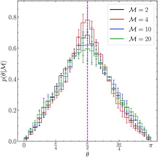
$The distribution of the angle, θ, between the local magnetic and velocity field for the ensemble of $\mathcal {M}_{\rm A0}=0.1$ simulations averaged over $5 \le t/T \le 7$.$

Figure A1.

The distribution of the angle, θ, between the local magnetic and velocity field for the ensemble of |$\mathcal {M}_{\rm A0}=0.1$| simulations averaged over |$5 \le t/T \le 7$|⁠.

Open in new tab Download slide

Note that in this sub-Alfvénic regime there is only a very small fluctuating component compared to the mean field, |${B}_0$| (see discussion in Section 4.3 in the main study). When we compute θ, the angle between |${B}$| and |$\delta {v}$| in each cell, because |${B}_0$| dominates the magnetic field, |${B}\approx {B}_0$|⁠, and hence |$\theta \approx \arccos \left[({v}\cdot {B}_0)/(\Vert {v} \Vert \Vert {B}_0\Vert)\right]$|⁠. This makes sense for our study since B₀ partitions our density domain into parallel and perpendicular components. However, since we are including |${B}_0$| in our θ, dynamic alignment theory (Boldyrev 2006; Matthaeus et al. 2008) does not apply, hence we urge caution when comparing Fig. A1 with other θ or cos θ distributions between the local magnetic and velocity fields.

Author notes

Einstein Fellow.

This article is published and distributed under the terms of the Oxford University Press, Standard Journals Publication Model (https://dbpia.nl.go.kr/journals/pages/open_access/funder_policies/chorus/standard_publication_model)

Download all slides

Month:	Total Views:
April 2021	6
May 2021	14
June 2021	21
July 2021	10
August 2021	21
September 2021	13
October 2021	17
November 2021	4
December 2021	3
January 2022	4
February 2022	5
March 2022	6
April 2022	22
May 2022	13
June 2022	16
July 2022	35
August 2022	30
September 2022	13
October 2022	17
November 2022	13
December 2022	6
January 2023	12
February 2023	8
March 2023	16
April 2023	15
May 2023	9
June 2023	13
July 2023	11
August 2023	12
September 2023	6
October 2023	12
November 2023	7
December 2023	11
January 2024	14
February 2024	20
March 2024	4
April 2024	16
May 2024	22
June 2024	21
July 2024	20
August 2024	17
September 2024	23
October 2024	26
November 2024	24
December 2024	9
January 2025	22
February 2025	8
March 2025	16
April 2025	8
May 2025	13

Article Contents

A multishock model for the density variance of anisotropic, highly magnetized, supersonic turbulence Free

ABSTRACT

1 INTRODUCTION

2 THE DENSITY PDF AND VARIANCE

2.1 Lognormal models

2.2 The relation between shocks and the density variance

3 DERIVING AN ANISOTROPIC DENSITY VARIANCE MODEL

3.1 Geometry of a shock

3.2 Shocks in MHD turbulence

3.2.1 Type I: hydrodynamic shocks

3.2.2 Type II: fast magnetosonic shocks

3.3 Two-shock density variance model

4 MHD SIMULATIONS

4.1 MHD model

4.2 Turbulent driving, density and velocity fields

4.3 Magnetic fields

5 IMPLEMENTATION OF THE ANISOTROPIC DENSITY VARIANCE MODEL

5.1 Volume fractions of anisotropic fluctuations

5.2 Determining the volume fraction of parallel and perpendicular fluctuations

6 ANISOTROPIC DENSITY VARIANCE MODEL RESULTS

6.1 Limiting behaviour of the model

7 DISCUSSION

7.1 Implications for density fluctuations observed in the ISM

7.2 Implications for star formation theory

8 SUMMARY AND KEY FINDINGS

ACKNOWLEDGEMENTS

DATA AVAILABILITY

Footnotes

REFERENCES

APPENDIX A: FLOW ORIENTATION IN THE SUB-ALFVÉNIC, SUPERSONIC REGIME

Author notes

Citations

Views

Altmetric

Email alerts

Astrophysics Data System

Citing articles via

Latest

Most Read

Most Cited

This Feature Is Available To Subscribers Only

A multishock model for the density variance of anisotropic, highly magnetized, supersonic turbulence