


ABSTRACT
We produce 1000 realizations of synthetic clustering catalogues for each type of the tracers used for the baryon acoustic oscillation and redshift space distortion analysis of the Sloan Digital Sky Surveys-iv extended Baryon Oscillation Spectroscopic Survey final data release (eBOSS DR16), covering the redshift range from 0.6 to 2.2, to provide reliable estimates of covariance matrices and test the robustness of the analysis pipeline with respect to observational systematics. By extending the Zel’dovich approximation density field with an effective tracer bias model calibrated with the clustering measurements from the observational data, we accurately reproduce the two- and three-point clustering statistics of the eBOSS DR16 tracers, including their cross-correlations in redshift space with very low computational costs. In addition, we include the gravitational evolution of structures and sample selection biases at different redshifts, as well as various photometric and spectroscopic systematic effects. The agreements on the auto-clustering statistics between the data and mocks are generally within |$1\, \sigma$| variances inferred from the mocks, for scales down to a few |$h^{-1}\, {\rm Mpc}$| in configuration space, and up to |$0.3\, h\, {\rm Mpc}^{-1}$| in Fourier space. For the cross correlations between different tracers, the same level of consistency presents in configuration space, while there are only discrepancies in Fourier space for scales above |$0.15\, h\, {\rm Mpc}^{-1}$|. The accurate reproduction of the data clustering statistics permits reliable covariances for multi-tracer analysis.
1 INTRODUCTION
The spatial clustering of large-scale structures (LSS) offers insights into the expansion history of the Universe and the growth of structures. In particular, the baryon acoustic oscillation (BAO; Eisenstein & Hu 1998) feature is known as a standard ruler for geometrical measurements and provides constraints on the nature of dark energy (Eisenstein 2005). Redshift-space distortions (RSD; Kaiser 1987) of the clustering statistics can be used to estimate the structure formation rate and test gravity theories (Percival & White 2009; Raccanelli et al. 2013). Precise cosmological constraints with clustering measurements require the 3D positions – 2D angular position and redshift – of tracers of the dark matter density field over a large volume, and possibly several different types of tracers to probe different cosmic epochs.
Recent large-scale galaxy spectroscopic surveys, such as the Baryon Oscillation Spectroscopic Survey (BOSS; Dawson et al. 2013) – which belongs to the phase iii of the Sloan Digital Sky Surveys (SDSS) – have measured the redshifts of over one million luminous red galaxies (LRG) with redshifts up to 0.75, covering more than 9000 deg2, and achieved per cent-level measurements of both distance scales and growth rate of structures (Alam et al. 2017). In addition, the extended BOSS (eBOSS; Dawson et al. 2016), as part of SDSS-iv (Blanton et al. 2017) and a complement to BOSS, has probed ∼0.8 million LRGs, star-forming emission line galaxies (ELG), and quasi stellar objects (QSO) in total, with the redshift range 0.6 < z < 2.2, for the LSS analysis of its final data release (DR16, see Section 2.1; Ross et al. 2020; Raichoor et al. 2021). In addition, ∼0.2 million BOSS/eBOSS QSOs at z > 2.1 are used for Lyman-α absorption measurements (du Mas des Bourboux et al. 2020; Lyke et al. 2020), which extend the clustering analysis to higher redshift.
Apart from the sample size, accurate estimates of the uncertainties in the clustering statistics are also essential for LSS analysis. One can obtain the covariance matrices directly from the observational catalogues, by sampling the data in subvolumes with jackknife or bootstrap estimations. However, variances on scales larger than the size of the subvolumes cannot be sampled, and systematic errors that apply to all subsamples are not accounted for. An alternative way is to rely on the theoretical model for clustering statistics, and derive Gaussian covariances (e.g. Grieb et al. 2016; Wadekar & Scoccimarro 2019). Further improvements can be achieved by rescaling the shot noise power to include non-Gaussianity (Philcox et al. 2020). Nevertheless, the robustness of analytical approaches depend on the accuracies of the models in nonlinear regimes of the cosmic evolution, and it is challenging for them to include observational systematic errors.
In principle, these issues can be solved with catalogues generated by N-body simulations: they encode the full nonlinear gravitational evolution, and can be applied known observational effects to sample systematic errors. However, the estimate of covariance matrices requires a large number of realizations, and this is generally too computational expensive to be practical for N-body simulations with sufficient mass resolution and volume for current large-scale galaxy surveys. To circumvent this problem, some more efficient but less accurate methods for constructing mock catalogues are proposed, such as the bias assignment method (BAM; Balaguera-Antolínez et al. 2019), COmoving Lagrangian Acceleration (COLA; Tassev, Zaldarriaga & Eisenstein 2013; Izard, Crocce & Fosalba 2016; Koda et al. 2016), effective Zel’dovich approximation mock (EZmock; Chuang et al. 2015a), FastPM (Feng et al. 2016), GaLAxy Mocks (GLAM; Klypin & Prada 2018), lognormal (Coles & Jones 1991; Agrawal et al. 2017), peak patch (Bond & Myers 1996; Stein, Alvarez & Bond 2019), PerturbAtion Theory Catalog generator of Halo and galaxY distributions (PATCHY; Kitaura, Yepes & Prada 2014), and quick particle mesh (QPM; White, Tinker & McBride 2014).
These fast mock generation methods can be classified into three general categories. COLA, FastPM, GLAM, peak patch, and QPM are predictive algorithms that solve the dynamic evolution of structures approximately. BAM, EZmock, and PATCHY generate the dark matter density field using perturbation theories, and then populate tracers with effective descriptions of their biases. While the lognormal method models halo distributions through modifications of the matter density field. In particular, comparisons of some of the mock construction techniques with N-body simulations have shown that methods with bias models, including EZmock and PATCHY, are not only among the most accurate ones, but also significantly faster than methods with comparable precisions (Chuang et al. 2015b; Blot et al. 2019; Colavincenzo et al. 2019; Lippich et al. 2019). Actually, PATCHY has been used for the BOSS DR12 analyses (e.g. Kitaura et al. 2016; Alam et al. 2017). We choose EZmock for this work, due to its higher efficiency, and fewer free parameters of the bias model, which makes it easier to be calibrated.
The EZmock algorithm uses Zel’dovich approximation (Zel’dovich 1970) to construct the density field at a given redshift, and populate matter tracers (haloes/galaxies/quasars) in the field with a parametrized modelling of tracer bias. This effective bias description includes linear, nonlinear, deterministic and stochastic effects, which have to be calibrated with clustering statistics from observations or N-body simulations, including typically the two-point correlation function (2PCF), power spectrum, and bispectrum. EZmock is able to reproduce both two- and three-point statistics of a reference N-body simulation precisely down to mildly nonlinear scales. For instance, the discrepancies of redshift space power spectrum produced by EZmock are less than 5 per cent for |$k \lesssim 0.3\, h\, {\rm Mpc}^{-1}$| (Chuang et al. 2015b). Moreover, thanks to the incomparable efficiency of ZA, the remarkably low computational cost makes EZmock extremely suitable for estimating covariances for large-scale analysis.
In this work, we use the revised EZmock method to construct mock catalogues for all eBOSS direct LSS tracers, including LRGs, ELGs, and QSOs. For the estimates of the covariance matrices, we produce 1000 realizations of mock catalogues for each type of the tracers. They are constructed from 46 000 simulation boxes with the side length of |$5\, h^{-1}\, {\rm Gpc}$|, at several different redshifts, to account for the redshift evolution of structures. Furthermore, the mock tracers are populated from shared density fields, to ensure reliable estimates of the cross covariances. Besides, two sets of mocks are generated, complete and realistic, i.e. without and with applying observational systematic effects. They are used for the analysis of the eBOSS LRG samples (Gil-Marín et al. 2020; Bautista et al. 2021), ELG samples (Tamone et al. 2020; de Mattia et al. 2021; Raichoor et al. 2021), QSO samples (Neveux et al. 2020; Hou et al. 2021), and the final cosmological constraints (eBOSS Collaboration 2020), with the systematic errors assessed using N-body simulations (Alam et al. 2020a; Avila et al. 2020; Rossi et al. 2020; Smith et al. 2020). Moreover, Lin et al. (2020) use the GLAM method to construct the density field and adopt the bias model of the QPM method to generate mock catalogues for eBOSS ELGs. The eBOSS DR16 EZmock catalogues presented in this work will be publicly available.1 In addition, all SDSS BAO and RSD measurements and the cosmological interpretations can be found on the SDSS website.2
This paper is organized as follows. In Section 2, we describe the methodology for constructing the mock catalogues. The clustering statistics of the mock catalogues are shown in Section 3. We perform the cross correlation analysis between different tracers in Section 4. Finally, in Section 5, we present the conclusions.
2 METHODOLOGY
We present in this section the improved version of the EZmock method, compared to the algorithm introduced in Chuang et al. (2015a). In particular, the method used for this work does not require the enhancement of the BAO signal for the initial conditions, and relies on less bias parameters to be calibrated. Moreover, the calibration is done directly with the observed clustering measurements of the BOSS and eBOSS catalogues, without taking N-body simulations as references. This is because no reliable N-body simulation multi-tracer catalogue is available when the mocks are constructed, and the accuracy of the EZmock method has been validated using the BigMultiDark simulation (Chuang et al. 2015b). As the result, the effective bias model of EZmock further accounts for the halo occupation distributions (HOD; e.g. Berlind & Weinberg 2002) of different matter tracers. We have made the python interface for constructing and calibrating EZmock catalogues publicly available.3
2.1 Reference data catalogues
The sky coverage of the BOSS DR12 and eBOSS DR16 data, with various masks applied, are illustrated in Fig. 1,4 where the background colour map indicates the angular source density of the Gaia DR2 public data (Gaia Collaboration 2018), with a selection of the g band magnitude (phot_g_mean_mag < 15). In particular, the left and right patches of the BOSS/eBOSS footprints are dubbed northern and southern Galactic caps (NGC and SGC) respectively. Since the two Galactic caps are spatially far away from each other, we construct EZmock catalogues for NGC and SGC independently, but with the same input parameters. Therefore, the expected clustering statistics of EZmock catalogues in both Galactic caps are identical, if no radial selection (see Section 2.3.4) is applied.
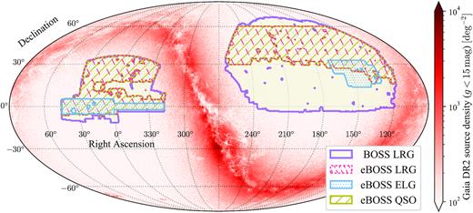
The sky coverage of eBOSS DR16 tracers and BOSS DR12 LRGs, as well as the density map of Gaia DR2 sources with |$g \lt 15\, {\rm mag}$|.
The total effective area of the CMASS LRG, eBOSS LRG, eBOSS ELG, and eBOSS QSO samples is 9376, 4103, 727, and 4702 deg2, respectively (Reid et al. 2016; Ross et al. 2020; Raichoor et al. 2021). The effective overlapped area between the eBOSS LRG and ELG samples is 458 deg2, and it is 509 deg2 for the overlapping region between eBOSS ELG and QSO samples.
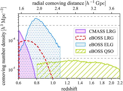
The weighted comoving number densities of eBOSS DR16 tracers and BOSS DR12 CMASS LRGs, with all the photometric and spectroscopic systematic weights included. The comoving distances and volumes are evaluated in the flat ΛCDM cosmology with Ωm = 0.31. The three horizontal dashed lines show the number densities of the cubic LRG, ELG, and QSO EZmock catalogues, i.e. 3.2 × 10⁻⁴, 6.4 × 10⁻⁴, and |$2.4 \times 10^{-5}\, h^3\, {\rm Mpc}^{-3}$|, respectively.
Since all BOSS and eBOSS tracers share the sky area and redshift range to some extent, in order to combine their results for final cosmological analysis, it is crucial to account for the cross covariance between different tracers. To this end, we construct the mock catalogues for different tracers – including BOSS CMASS LRGs, and eBOSS LRGs/ELGs/QSOs – in the same comoving volume, and with identical initial conditions, to ensure the same underlying dark matter density field for all of them.
2.2 Cubic mock catalogue generation
The starting point of our mock generation process is a Gaussian random field in a periodic cubic volume, with a given initial power spectrum. The side length of the Gaussian random field in this work is |$5\, h^{-1}\, {\rm Gpc}$|, which is large enough to cover the survey volume of all tracers for clustering analysis. The same white noises are used for the construction of the Gaussian random field for different tracers.
The fiducial cosmological model for constructing the mocks is flat ΛCDM, with Ωm = 0.307115, Ωb = 0.048206, h = 0.6777, σ8 = 0.8225, and ns = 0.9611, which are the best-fitting values from the Planck 2013 results (Planck Collaboration 2014). This is the same cosmological model used by the patchy mock catalogues for the final BOSS data release (Kitaura et al. 2016) which is calibrated based on the MultiDark simulations (Klypin et al. 2016). The linear matter power spectrum we use is generated by the camb5 software (Lewis, Challinor & Lasenby 2000). It has been shown that the covariance matrix of two-point clustering measurements are insensitive to the input power spectrum, if the two- and three-point statistics of the mocks are consistent with the observed measurements (Baumgarten & Chuang 2018).
2.2.1 Zel’dovich approximation
Once the displacement field is computed on the grid points, dark matter particles are moved from their initial Lagrangian positions – Cartesian grid points – to the final Eulerian positions following equation (7). The dark matter density field is evaluated on the same grids, using the Cloud-in-Cell (CIC; Hockney & Eastwood 1981) particle assignment scheme. Consequently, the number density fields of the observational tracers described hereafter, are all based on this grid size. In general, the EZmock parameters have to be re-calibrated, with a different number of grids in the same comoving volume.
2.2.2 Deterministic bias relations
To implement equation (12) for the mock tracers, we begin with some analytical bias relations that have been confirmed with N-body simulations. However, due to the inaccuracy of ZA in the nonlinear regime, the analytical form of B is not enough for a precise bias model. The actual ρt is generated with a rank ordering process detailed in Section 2.2.4, in a numerical manner.
2.2.3 Stochastic bias relations
In general, the stochastic bias of galaxies is non-Poissonian and depends on the environments (Somerville et al. 2001; Casas-Miranda et al. 2002). Nevertheless, it is the order of tracer densities in different cells that matters in this work, rather than the actual functional form for the scatter. This is because the densities are further modified by rank ordering with a PDF mapping scheme detailed in the next subsection. For a more realistic description of stochastic biases, see the negative binomial distribution proposed by Kitaura et al. (2014), and further validated in Vakili et al. (2017); Pellejero-Ibañez et al. (2020).
In practice, the value of λ in equation (17) alters mainly the amplitude of the power spectrum and bispectrum, and the same effect can be achieved by the other parameters, such as ρc and ρexp, hence we set λ = 10 throughout this work.
2.2.4 PDF mapping scheme
We then map nc(nt) to the expected tracer number density ρt, which is estimated by the bias relations described in the previous sections, in descending order. For instance, we rank the cells by ρt, and assign nt, max tracers to nc(nt, max) cells with the highest ρt values, and then (nt, max − 1) tracers to the next nc(nt, max − 1) cells, etc. Thus, the exact values of ρt defined in equation (16) is irrelevant for our purpose, as they are effectively modified based on their orders.
The tracers are then assigned randomly to the dark matter particles in each grid cell, if there are any. For cells without enough number of dark matter particles, we randomly pick a position in the cell for the tracer, which potentially damps the BAO feature. However, this effect is subdominant in this work, as the fractions of LRGs, ELGs, and QSOs that are randomly placed, are only ∼ 6 per cent, 16 per cent, and 4 per cent respectively. Moreover, the strength of the BAO feature has little impacts on the covariance matrices, compared to the contribution of the broad-band amplitudes. Thus, the enhancement of the BAO feature in the input power spectrum introduced by Chuang et al. (2015a), for correcting the BAO smearing due to the smooth galaxy distribution inside grid cells, is no longer necessary.
2.2.5 Redshift space distortions
2.2.6 Summary of model parameters
So far we have introduced six EZmock parameters for the effective modelling of tracer biases, and they are summarized in Table 1. Since some of the parameters are highly correlated, and we fix the density saturation ρsat and the width λ of the Gaussian random distribution for the stochastic biasing. Thus, there are four free parameters to be calibrated with the two- and three-point clustering statistics of the reference catalogues, i.e. the BOSS DR12 CMASS and eBOSS DR16 catalogues. In order to take into account the impact of survey geometry on the clustering statistics, we calibrate these free parameters only with the EZmock light-cone catalogues that mimic the geometry of eBOSS DR16 data.
Since the observational systematics affect mainly scales outside the range of clustering statistics for EZmock calibrations (see Section 2.5 for scales relevant for the calibration, and Section 3 for the comparison between complete and realistic mocks), and it is relatively computational expensive to apply observational effects to the mock catalogues, we calibrate the EZmock parameters with the complete set of EZmock light-cones, rather than the realistic ones. In practice, the calibration is done with a single mock realization by manually fine-tuning. The results are then validated using 50 realizations to eliminate impacts of cosmic variances, before the mass production.
2.3 Complete light-cone catalogue construction
To construct practical mock catalogues, various geometrical features of the observed data have to be applied to the cubic mocks. To this end, we use the make_survey6 toolkit (White et al. 2014) to rotate the cubic EZmock catalogues, map the tracers with observational coordinates, and trim the catalogues according to the survey footprints and veto masks defined by mangle7 (Swanson et al. 2008) polygon files. This procedure is similar to that of the SUrvey GenerAtoR code (sugar; Rodríguez-Torres et al. 2016) used for BOSS DR12 Patchy mocks (Kitaura et al. 2016).
2.3.1 Coordinate conversion
2.3.2 Survey volume trimming
To mimic the angular area of the BOSS DR12 CMASS and eBOSS DR16 data, we trim the EZmock catalogues with the BOSS/eBOSS footprints, which are defined by groups of sectors – regions covered by a unique set of plates (Ross et al. 2020) – in the mangle polygon format. To have reliable clustering measurements, the sectors are further selected according to the associate CeBOSS and Cz values – CeBOSS > 0.5 and Cz > 0.5 for LRGs and QSOs, and CeBOSS ≥ 0.5 and Cz ≥ 0 for ELGs – where CeBOSS denotes the fraction of targets that are assigned fibres, or without fibres only due to fibre-collision, and Cz indicates the proportion of valid tracers with fibres, for which a reliable redshift is obtained (see Ross et al. 2020; Raichoor et al. 2021, for more details).
In the radial direction, we simply select EZmock tracers with redshifts inside the redshift range of the corresponding BOSS/eBOSS data catalogues (see equations (1) – (3)). The comoving volume of the EZmock catalogues after survey volume trimming, compared to the original cubic periodic boxes, are shown in Fig. 3.8
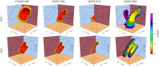
The comoving volume of EZmock catalogues after survey volume trimming, compared with the |$(5\, h^{-1}\, {\rm Gpc})^3$| periodic box for constructing the mocks. Regions with different colours indicate the redshift slices used for reproducing the redshift evolution of clustering statistics (see Section 2.3.5). The QSO sample in the NGC benefits from the periodic boundary conditions, as its comoving volume is too large to be placed inside the box.
2.3.3 Veto masks
Inside the survey volume there are still angular patches to be removed, such as fields that were not observed, or regions that are too close to bright object to have reliable redshift measurements. In general, the shapes and distributions of these masks depend on the brightness of the tracers, sources of the images, and the calibration process. The angular veto masks of the eBOSS DR16 and BOSS DR12 samples are shown in Fig. 4, where the colours indicate different types of masks, i.e. regions removed for different reasons (see Ross et al. 2020; Raichoor et al. 2021, for more details).
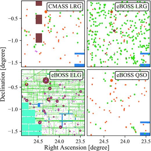
Angular veto masks for eBOSS DR16 tracers and BOSS DR12 CMASS LRGs, for the same patch of the sky. Tracers in the coloured regions are removed for various reasons, such as bright source contaminations or unreliable photometric measurements.
In practice, the LRG and QSO veto masks are encoded as mangle polygons, and can be simply applied with the mply_trim tool of the make_survey package. However, as can be seen in Fig. 4, the eBOSS ELG veto masks are much more complicated than those of the other tracers. Thus, it is not practical to translate the ELG masks to simple polygons. Instead, the mask information is associated with each pixel of the DECaLS bricks (Raichoor et al. 2021). We then use the brickmask9 code to apply the ELG masks, which is made publicly available.
2.3.4 Radial selection and FKP weighting
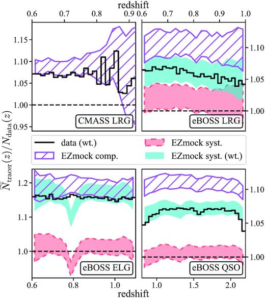
(Weighted) tracer distribution of the BOSS/eBOSS data and EZmock catalogues, normalized by the number of objects in the corresponding data catalogues. ‘EZmock comp.’ and ‘EZmock syst.’ denote the complete and realistic EZmock catalogues respectively, and ‘wt.’ indicates results evaluated with weights, which are the total photometric and spectroscopic weights used for clustering analyses. The upper and lower boundaries of the filled regions show the 1 σ deviation obtained from 1000 realizations of mocks.
2.3.5 Redshift slices
The redshift slices used in this work are listed in Table 2 (see also Fig. 3 for the illustration in comoving space). Catalogues generated at different effective redshifts are trimmed with the corresponding zlow and zhigh values, after performing coordinate conversions (Section 2.3.1). These slices are then combined to construct the sample in the full redshift range of the data. Finally, the survey footprint, veto masks, and radial selections (Sections 2.3.2 – 2.3.4) are all applied to the combined catalogues.
The final redshift slices for the production of EZmock catalogues, with the corresponding effective redshift (equation (35)) and (weighted) number of tracers from the observed data. Ndata denotes the number of objects in each redshift bin, and wi indicates the total photometric and spectroscopic systematic weights.
| Sample | zlow | zhigh | zeff | |$z_{\rm eff}^{(2)}$| | Ndata | |$\sum \limits _{ {i}}^{ {N_{\rm data}}} w_i$| |
|---|---|---|---|---|---|---|
| CMASS LRG | 0.6 | 0.65 | 0.626 | 0.392 | 114441 | 122385 |
| 0.65 | 0.7 | 0.675 | 0.455 | 57561 | 61461.9 | |
| 0.7 | 0.8 | 0.737 | 0.545 | 30899 | 33024.2 | |
| 0.8 | 1.0 | 0.847 | 0.719 | 2473 | 2643.8 | |
| eBOSS LRG | 0.6 | 0.65 | 0.625 | 0.391 | 28152 | 29983.1 |
| 0.65 | 0.7 | 0.675 | 0.456 | 33557 | 35828.4 | |
| 0.7 | 0.8 | 0.751 | 0.564 | 64460 | 68592.7 | |
| 0.8 | 0.9 | 0.847 | 0.719 | 37080 | 39099.7 | |
| 0.9 | 1.0 | 0.940 | 0.885 | 11567 | 12130.2 | |
| eBOSS ELG | 0.6 | 0.7 | 0.658 | 0.434 | 10046 | 11667.4 |
| 0.7 | 0.75 | 0.725 | 0.526 | 20275 | 23373.6 | |
| 0.75 | 0.8 | 0.775 | 0.601 | 33487 | 38857.9 | |
| 0.8 | 0.85 | 0.825 | 0.682 | 34631 | 40140.4 | |
| 0.85 | 0.9 | 0.876 | 0.767 | 27831 | 32231.0 | |
| 0.9 | 1.0 | 0.950 | 0.903 | 32721 | 37792.2 | |
| 1.0 | 1.1 | 1.047 | 1.097 | 14745 | 16997.8 | |
| eBOSS QSO | 0.8 | 1.0 | 0.907 | 0.826 | 35988 | 38026.4 |
| 1.0 | 1.2 | 1.104 | 1.223 | 47025 | 50276.2 | |
| 1.2 | 1.4 | 1.301 | 1.697 | 57120 | 61230.1 | |
| 1.4 | 1.6 | 1.500 | 2.252 | 55758 | 59573.2 | |
| 1.6 | 1.8 | 1.700 | 2.894 | 56678 | 60640.0 | |
| 1.8 | 2.0 | 1.898 | 3.606 | 50774 | 54310.4 | |
| 2.0 | 2.2 | 2.094 | 4.389 | 40357 | 42731.2 |
2.3.6 Sample combination
Since the BOSS DR12 CMASS and eBOSS DR16 LRG samples overlap widely in both angular and radial directions (see Figs 1 and 2), and they consist of the same type of galaxies (Prakash et al. 2016; Reid et al. 2016), it is reasonable to combine the two datasets directly for joint clustering analyses. Nevertheless, special care has to be taken since the footprint of the two samples are not identical. We follow the combination procedure described in Ross et al. (2020) for the observational data. In brief, we detect eBOSS LRG sectors that contain CMASS LRGs, and add their comoving number densities in redshift bins, with the bin size of Δz = 0.01, to obtain the number density of the combined sample. The FKP weights are then revised accordingly, following equation (31). By contrast, eBOSS galaxies in sectors that do not contain CMASS objects, and CMASS galaxies outside eBOSS sectors, are not altered.
Moreover, when combining CMASS and eBOSS EZmock catalogues, we have ensured that they are constructed with the same initial conditions. This restriction is also applied for the combination of redshift slices, or ELG chunks.
2.4 Random catalogue creation
In order to account for the survey window function, including the radial number density of tracers, random catalogues are required for clustering measurements. One simple way to generate random catalogue for EZmock catalogues is to apply the light-cone catalogue creation procedure described in Section 2.3 (except the redshift division in Section 2.3.5, as there is no evolution for a random catalogue), to a uniform random sample in comoving space. In this case, a single random catalogue is necessary for each type of the tracers in individual Galactic caps.
However, the radial selection function of the BOSS DR12 CMASS and eBOSS DR16 catalogues are not directly sampled from the number density of data. Instead, redshifts of the observed data are shuffled, and randomly assigned to the angular random catalogues (Reid et al. 2016; Ross et al. 2020; Raichoor et al. 2021). This is because the true redshift distribution of data is usually complicated and unknown, since it depends on various imaging and spectroscopic effects. Indeed, the comoving number density shown in Fig. 2 is only a binned estimation of the true radial selection function, whereas, the shuffled approach ensures the correct radial distribution of random objects automatically. Nevertheless, this method introduces a radial effect that is similar to an additional window function, and bias the clustering measurements on large scales significantly (de Mattia & Ruhlmann-Kleider 2019). To investigate this problem, we create also random catalogues for the mocks with the shuffled method.
In practice, we generate firstly the random catalogue with redshifts sampled from the spline interpolation of the comoving number density measured from the BOSS/eBOSS data, as is done in Section 2.3.4. And we dub them the ‘sampled’ random catalogues. Then, we keep only the angular positions of these random catalogues, and randomly assign the shuffled redshifts of the EZmock catalogues to the angular random positions, to create the ‘shuffled’ random catalogues. Note that there is one ‘shuffled’ random catalogue for each of the EZmock realizations. The consequences of the two sets of random catalogues are shown in Section 3.
2.5 EZmock parameter calibration
We aim at encoding redshift evolution in the EZmock light-cone catalogues. To this end, besides constructing mocks at different effective redshifts, the effective bias model of EZmock has to be adjusted for each of the redshift slices. This requires individual calibrations of EZmock parameters (see Table 1) for each bin, with the clustering of observed data catalogues measured in corresponding redshift ranges. However, for many of the redshift bins listed in Table 2, the number of tracers are too low for precise measurements of two- and three-point statistics from the observational data, and the calibration results may be dominated by statistical noise.
To circumvent this problem, we use larger but overlapping redshift bins to determine the EZmock parameters, as shown in Table 2. When calibrating EZmock parameters for each bin, we compare the following clustering statistics measured from the complete EZmock light-cone catalogues for both NGC and SGC, with the ones obtained from BOSS/eBOSS data:
ξ0(s), ξ2(s): 2PCF monopole and quadrupole, with the galaxy pair separation range of |$s \in [10, 50]\, h^{-1}\, {\rm Mpc}$|.
P0(k), P2(k): power spectrum monopole and quadrupole, with the Fourier mode range of |$k \in [0.1,0.3]\, h\, {\rm Mpc}^{-1}$| (apart from eBOSS QSO NGC, which is only calibrated on scales up to |$k \sim 0.24\, h\, {\rm Mpc}^{-1}$|, see Section 3.3.1).
B(k1, k2, θ12): bispectrum, with |$k_1 = 0.1 \pm 0.01\, h\, {\rm Mpc}^{-1}$|, |$k_2 = 0.05 \pm 0.01\, h\, {\rm Mpc}^{-1}$|, and θ12 being the angle between |$\boldsymbol{k}_1$| and |$\boldsymbol{k}_2$|.
In particular, the ranges of the two-point statistics are chosen to be nonsensitive to observational systematic effects, and the same EZmock parameters are used for the two Galactic caps.
The redshift slices used for the calibration of EZmock catalogues, with the corresponding effective redshift (equation (35)) and (weighted) number of tracers from the observed data. Ndata denotes the number of objects in each redshift bin, and wi indicates the total photometric and spectroscopic systematic weights.
| Sample | zlow | zhigh | zeff | |$z_{\rm eff}^{(2)}$| | Ndata | |$\sum \limits _{ {i}}^{ {N_{\rm data}}} w_i$| |
|---|---|---|---|---|---|---|
| CMASS LRG | 0.6 | 0.7 | 0.652 | 0.426 | 172002 | 183847 |
| 0.65 | 0.75 | 0.696 | 0.485 | 81206 | 86695.2 | |
| 0.7 | 0.8 | 0.737 | 0.545 | 30899 | 33024.2 | |
| 0.75 | 1.0 | 0.791 | 0.628 | 9727 | 10434.8 | |
| eBOSS LRG | 0.6 | 0.7 | 0.652 | 0.426 | 61709 | 65811.5 |
| 0.65 | 0.8 | 0.727 | 0.531 | 98017 | 104421 | |
| 0.7 | 0.9 | 0.797 | 0.638 | 101540 | 107692 | |
| 0.8 | 1.0 | 0.878 | 0.773 | 48647 | 51229.9 | |
| eBOSS ELG | 0.6 | 0.8 | 0.714 | 0.512 | 63808 | 73898.9 |
| 0.7 | 0.9 | 0.805 | 0.651 | 116224 | 134603 | |
| 0.8 | 1.0 | 0.905 | 0.821 | 95183 | 110164 | |
| 0.9 | 1.1 | 0.994 | 0.991 | 47466 | 54790 | |
| eBOSS QSO | 0.8 | 1.3 | 1.077 | 1.181 | 110950 | 118238 |
| 1.1 | 1.5 | 1.305 | 1.717 | 110326 | 118197 | |
| 1.3 | 1.7 | 1.499 | 2.262 | 113477 | 121358 | |
| 1.5 | 1.9 | 1.699 | 2.899 | 110370 | 117993 | |
| 1.7 | 2.2 | 1.930 | 3.747 | 65077 | 69150.3 |
The calibrated EZmock parameters for different redshift slices, that are used for both NGC and SGC.
| Sample | zlow | zhigh | ρc | ρexp | b | ν |
|---|---|---|---|---|---|---|
| CMASS LRG | 0.6 | 0.65 | 0.90 | 2.80 | 0.240 | 175 |
| 0.65 | 0.7 | 1.14 | 3.84 | 0.249 | 175 | |
| 0.7 | 0.8 | 1.37 | 4.19 | 0.252 | 175 | |
| 0.8 | 1.0 | 1.55 | 3.88 | 0.251 | 175 | |
| eBOSS LRG | 0.6 | 0.65 | 0.35 | 2.50 | 0.180 | 190 |
| 0.65 | 0.7 | 0.63 | 3.46 | 0.205 | 190 | |
| 0.7 | 0.8 | 0.80 | 3.00 | 0.220 | 190 | |
| 0.8 | 0.9 | 1.05 | 3.79 | 0.257 | 190 | |
| 0.9 | 1.0 | 0.93 | 4.40 | 0.295 | 190 | |
| eBOSS ELG | 0.6 | 0.7 | 0.50 | 1.00 | 0.181 | 150 |
| 0.7 | 0.75 | 0.50 | 1.00 | 0.180 | 150 | |
| 0.75 | 0.8 | 0.50 | 1.00 | 0.186 | 150 | |
| 0.8 | 0.85 | 0.50 | 1.00 | 0.195 | 150 | |
| 0.85 | 0.9 | 0.50 | 1.00 | 0.211 | 150 | |
| 0.9 | 1.0 | 0.50 | 1.00 | 0.243 | 150 | |
| 1.0 | 1.1 | 0.50 | 1.00 | 0.300 | 150 | |
| eBOSS QSO | 0.8 | 1.0 | 1.00 | 0.47 | 0.0100 | 200 |
| 1.0 | 1.2 | 0.88 | 0.66 | 0.0089 | 217 | |
| 1.2 | 1.4 | 0.57 | 0.81 | 0.0057 | 330 | |
| 1.4 | 1.6 | 0.41 | 0.92 | 0.0033 | 415 | |
| 1.6 | 1.8 | 0.37 | 0.99 | 0.0017 | 474 | |
| 1.8 | 2.0 | 0.49 | 1.02 | 0.0010 | 501 | |
| 2.0 | 2.2 | 0.74 | 1.01 | 0.0011 | 501 |
2.6 Observational effects
The complete set of EZmock catalogues do not present the inhomogeneity of the angular distribution of tracers due to various observational effects, e.g. the quality of photometric and spectroscopic data. These effects are typically treated as systematics, and are (partially) corrected by imaging and spectroscopic weights (e.g. Ross et al. 2020; Raichoor et al. 2021). To account for their impacts on the covariance matrices for clustering measurements, we generate more realistic EZmock catalogues by introducing observational effects to the complete mocks for eBOSS DR16 tracers.
2.6.1 Depth dependent radial density
For the eBOSS ELG EZmock catalogues, we start from the complete realizations before applying radial selection (see Section 2.3.4). This is because the imaging depth of the DECaLS data used for eBOSS ELG target selection is not homogenous inside eBOSS chunks, especially for eboss23, resulting in an imaging depth dependent number density of ELGs (Raichoor et al. 2017). This effect is migrated to the EZmock catalogues by the same strategy for generating the random catalogues for the observed data (see Raichoor et al. 2021). Basically the g-, r-, and z-band imaging depths are combined linearly, and the radial number densities of ELGs are evaluated inside three quantiles of the combined depth, for each eBOSS chunk. The EZmock ELGs are then split into the quantiles, and applied radial selections separately. In this case, the actual radial density of ELGs is anisotropic, and cannot be described by a simple redshift-dependent function. Consequently, the random catalogues for the realistic ELG EZmock catalogues are generated using the ‘shuffled’ scheme, by taking redshifts of galaxies in the quantiles separately.
2.6.2 Angular photometric systematics
Anisotropic effects that the photometric process carries, such as stellar density, Galactic extinction, seeing, and imaging depth, are correlated with the angular distributions of the samples for large-scale analysis (e.g. Ross et al. 2017; Xavier et al. 2019). To mimic these effects in EZmock catalogues, we extract an angular map of the photometric properties from the imaging sample, and randomly discarding mock tracers with the probability following this map. For LRGs and QSOs, the map is generated by linear regressions for different photometric effects (Ross et al. 2020), while for ELGs we use directly a smoothed angular target density map of the data, with a beam size of 1 deg (de Mattia et al. 2021). The corrections are then done by adding photometric weights to the mocks, which are estimated by linear regressions to the angular completeness (see Ross et al. 2020; Raichoor et al. 2021, for details) for each mock realization individually, thus allowing stochasticity for the systematic weights.
2.6.3 Fibre collision
Due to the finite size of optical fibres, the spectra of two targets with the angular separation less than 62 arcsec cannot be both measured with one plate. Thus, one of the targets has to be rejected if they do not reside in sectors covered by different plates.
We use the angular friends-of-friends (FoF) algorithm provided in the nbodykit11 (Hand et al. 2018) package, to detect groups of EZmock tracers that are in collision, and mark objects to be removed. Then, the groups are distributed to the sectors of the observational data, and some of the collisions can be resolved when the objects are in sectors belonging to multiple plates.
To correct the clustering statistics with fibre collision, remaining mock tracers in collision groups are up-weighted by the ratio between the original number of targets, and the number of assigned fibres, for each of the groups (cf. Hou et al. 2021, for more investigations on the fibre collision weights). The fibre collision effects on the configuration space measurements can be further suppressed by the pairwise-inverse-probability (PIP) weighting scheme, which is an unbiased procedure for all scales (Mohammad et al. 2020).
2.6.4 Redshift failure
Reliable redshifts are not always obtained from the spectra in practice. The redshift failure rate ffail for the eBOSS data are modelled by regressions with the signal-to-noise ratio of the spectra, as well as IDs and positions on the focal plane of optical fibres (Ross et al. 2020; Raichoor et al. 2021). This effect is introduced to the EZmock catalogues with a similar approach for eBOSS DR14 LRG QPM mocks (Bautista et al. 2018). We associate EZmock objects with the fibre of the closest valid eBOSS tracer, and randomly down-sample mocks according to the modelled redshift failure rate of the data. We then use the same procedure as with the data to fit our model for ffail for each individual mock, and the remained mock tracers are up-weighted by 1/(1 − ffail).
3 RESULTS: STATISTICAL COMPARISON BETWEEN EZMOCK CATALOGUES AND BOSS/EBOSS DATA
We generate 1000 realizations of EZmock catalogues, for each of the dataset, i.e. BOSS DR12 CMASS LRG, and eBOSS DR16 LRG/ELG/QSO. Thus, 46,000 EZmock boxes are generated, with the side length of |$5\, h^{-1}\, {\rm Gpc}$|, for the 23 redshift slices listed in Table 2, and both northern and southern Galactic caps. The number of tracers for each of the LRG, ELG, and QSO boxes are 4 × 10⁷, 8 × 10⁷, and 3 × 10⁶, respectively. It takes ∼1 million CPU hours in total, to generate the complete set of EZmock mock light-cone catalogues, on the Cori Haswell nodes of the National Energy Research Scientifc Computing Center (NERSC).12 The ezmock code is parallelized with OpenMP, and multiple realizations are run simultaneously with the jobfork13 tool, which distributes serial or OpenMP based jobs to multiple computing nodes using MPI.
In this section, we present various statistical properties of the EZmock catalogues and compare them with those from the BOSS/eBOSS data. In particular, results of both the complete and realistic mocks are shown. Moreover, we measure the clustering statistics for the complete mocks with both the ‘sampled’ and ‘shuffled’ random catalogues, and the results are denoted by ‘EZmock comp.’ and ‘EZmock R-shuf.’, respectively. While results for the realistic mocks are always obtained using the ‘shuffled’ random catalogues (denoted by ‘EZmock syst.’). Note however that the realistic joint BOSS and eBOSS LRG samples (denoted by ‘COMB BOSS’) are constructed with the combination of the complete CMASS LRG mocks and realistic eBOSS LRG mocks. The meanings of these notations are summarized in Table 5.
A list of notations for different EZmock samples.
| Notation | Description |
|---|---|
| EZmock comp. | Complete mocks with ‘sampled’ randoms: no observational systematics, and redshifts of the random catalogues are sampled from the spline interpolation of the n(z) of observational data. |
| EZmock R-shuf. | Complete mocks with ‘shuffled’ randoms: no observational systematics, and redshifts of the random catalogues are taken randomly from the corresponding data catalogues. |
| EZmock syst. | Realistic mocks with ‘shuffled’ randoms: all known observational systematics are applied to the data and random catalogues, and redshifts of the random catalogues are taken randomly from the corresponding data catalogues. |
Note that the clustering measurements of the complete mocks are used for EZmock parameter calibration (see Section 2.5), while the covariance matrices of the realistic mocks are our final products for the data analyses. The fiducial cosmological model used for coordinate conversion hereafter, is flat ΛCDM with Ωm = 0.31 (see equations (25) – (28)).
3.1 Spatial distribution
The radial distributions of the complete EZmock catalogues in comoving space follows those measured from the data with all photometric and systematic weights by construction (see equation (30)). However, the fraction of targets without fibres (C(e)BOSS; see Reid et al. 2016; Ross et al. 2020) are not considered by the weights. Thus, there can be discrepancies on the actual weighted radial counts between data and the corresponding mocks. This can be seen in Fig. 5, where the comparisons between EZmock tracers and BOSS/eBOSS data are shown, in terms of the (weighted) number of objects at different redshifts.
For the eBOSS samples, the number of targets without fibres is about 3.4 per cent of the total weighted number of LRGs, and the fractions are 0.9 and 2.3 per cent for ELGs and QSOs respectively. These numbers are consistent with the mismatch between EZmock catalogues and eBOSS data illustrated in Fig. 5. This effect is due to the definition of the effective area for measuring ndata, and for sectors with C(e)BOSS = 1, the radial comoving number density of tracers from the mocks and data are still consistent (see Appendix A for more discussions).
To have accurate estimates of the clustering covariance matrices, it is necessary to reproduce faithfully the sample size of the observational data. Hence, the effect of CeBOSS is considered in the realistic EZmock catalogues. Moreover, after including both photometric and spectroscopic effects (see Section 2.6), a considerable fraction of the mock tracers are removed. Consequently, the number of objects in the mocks and data become more comparable, though they are still not identical, since the small-scale clustering of EZmock catalogues does not allow precise reproduction of some of the observational systematics, such as fibre collision. Finally, the systematics of the realistic EZmock catalogues are corrected by various weights. Thus, the weighted redshift distribution of mocks and data agree well again, as shown in Fig. 5.
Furthermore, since the number density of the cubic EZmock ELG catalogues (|$6.4\times 10^{-4}\, h^3\, {\rm Mpc}^{-3}$|) are only slightly larger than the peak density of the eBOSS data in chunk eboss22, after down-sampling with observational systematics, the density of EZmock ELGs at z ∼ 0.8 are lower than that of the eBOSS data by at most 5 per cent. We then rescale the radial selection function (see Section 2.3.4) of ELGs in chunk eboss22, to obtain the correct number of objects in the full sample. Since this affects only a small number of EZmock ELGs, the consequences on the covariance matrices are sub-dominant.
Fig. 6 shows that angular systematic map extracted from the eBOSS DR16 data – including all the effects discussed in Section 2.6 – as well as the comparison of the unweighted angular tracer density between the data and one arbitrary EZmock realization. Note however that for better illustration, veto masks due to bad photometric calibrations are not shown for ELG SGC (cf. Raichoor et al. 2021). The large-scale angular distribution of both data and EZmock catalogues agree well with the systematic map: for regions with low completeness, the tracer densities are also low. Moreover, the small-scale clustering pattern of the data and mocks are also similar. We shall compare the clustering statistics quantitatively in the next section.
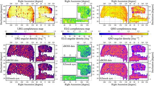
Top panel: angular completeness map of eBOSS DR16 tracers, modelled with the observational effects discussed in Section 2.6. Bottom panel: angular density distribution of tracers in the eBOSS data (first row), and one realization of EZmock catalogues with observational systematics (second row).
3.2 Configuration space clustering
3.2.1 2D two-point correlation function
The 2D 2PCF of the BOSS DR12 and eBOSS DR16 data, as well as the corresponding EZmock catalogues, are shown in Fig. 7. In particular, the colour plots show ξ(s∥, s⊥) for single catalogues, while the contour lines for the mocks indicate levels (see the colour bars) of the mean results obtained from all the 1000 mock realizations, and pair counts for both Galactic caps are combined. On scales smaller than |$\sim 120\, h^{-1}\, {\rm Mpc}$|, the results from the mocks are generally consistent with those of the data.
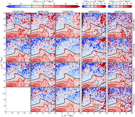
2D two-point correlation function ξ(s∥, s⊥) of the BOSS/eBOSS data (first row), the complete (second and third rows for the ‘sampled’ and ‘shuffled’ random catalogues respectively) and realistic (fourth row) EZmock catalogues. Only the first quadrant is shown, since ξ(s∥, s⊥) is symmetric about both s∥ = 0 and s⊥ = 0. Pair counts for NGC and SGC are combined. ‘COMB LRG’ denotes the joint sample with both BOSS and eBOSS LRGs. The colour plots are obtained from single realizations, while the contour lines indicate the averaged results of all the mocks. In particular, in the first row, the contour lines for the CMASS sample are computed from the complete mocks with ‘shuffled’ randoms, while for the other samples they are obtained using the realistic mocks.
By using the ‘shuffled’ random catalogues, the 2PCFs are suppressed when s∥ is small, especially for ELGs. The effect is more obvious on large s⊥, as the 2PCFs are rescaled by s2. This is because the data and random have common redshifts, resulting in a higher chance to find data–random pairs with s∥ ∼ 0, compared to the case with ‘sampled’ random catalogues. The 2PCFs are then reduced according to the Landy–Szalay estimator (equation (37)). Moreover, since the angular area of the ELG distribution is smaller, this effect starts to be evident from smaller scales.
The impacts of observational effects are also more significant for ELGs, due to the relatively more complicated sources of systematics (see Raichoor et al. 2021, for details). Apart from distortions on BAO scale, we also observe excess clustering strength on small angular scales (s⊥ ∼ 0).
3.2.2 Two-point correlation function multipoles
For the BOSS/eBOSS data and EZmock catalogues, we compute the 2PCF monopole (ℓ = 0), quadrupole (ℓ = 2), and hexadecapole (ℓ = 4), with 240 μ bins from −1 to 1, and 40 s bins from 0 to |$200\, h^{-1}\, {\rm Mpc}$|, and the results are shown in Figs 8 and 9, for NGC and SGC, respectively. On scales down to |$\sim 10\, h^{-1}\, {\rm Mpc}$|, the 2PCF multipoles of the observational data are well recovered by the corresponding EZmock catalogues, especially for the realistic mocks. Indeed, deviations over 1 σ are mainly observed on fairly large scales (|$s \gtrsim 150\, h^{-1}\, {\rm Mpc}$|), where the impact of observational systematics are relatively more obvious. A quantitative consistency check between the data and mocks is done in Section 3.5.
Two-point correlation function multipoles of the BOSS/eBOSS data and the corresponding EZmock catalogues in NGC. The solid/dashed envelopes and shadowed areas indicate the 1 σ regions evaluated from 1000 mock realizations. The error bars for the CMASS LRG sample are obtained from the complete EZmock catalogues, while for the other tracers they are taken from the realistic mocks with systematics.
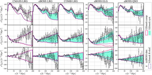
Two-point correlation function multipoles of the BOSS/eBOSS data and the corresponding EZmock catalogues in SGC. The solid/dashed envelopes and shadowed areas indicate the 1 σ regions evaluated from 1000 mock realizations. The error bars for the CMASS LRG sample are obtained from the complete EZmock catalogues, while for the other tracers they are taken from the realistic mocks with systematics.
Furthermore, the 2PCFs measured from the ‘sampled’ and ‘shuffled’ random catalogues differ mainly in the quadrupole and hexadecapole. This is because the differences are only found at fairly small s∥. Thus they are more obvious in anisotropic multipole measurements. Besides, observational systematic effects do not play important roles on the 2PCF multipoles for LRGs and QSOs. While for ELGs their impacts are significant.
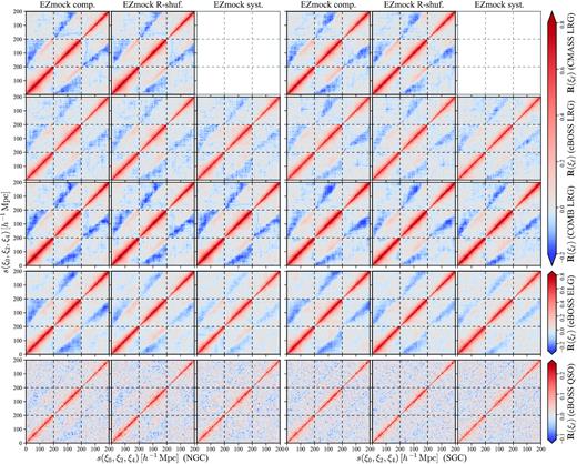
Correlation matrices of two-point correlation function multipoles obtained from 1000 EZmock realizations.
3.3 Fourier space clustering
To obtain the tracer density field, the data and random catalogues are placed into cuboids with adaptive side lengths. Note however that given a specific tracer sample, the size of cuboids for the observational data and the corresponding mocks are identical. Besides, we distribute tracers to 3D regular grids using the triangular shaped cloud (TSC; Hockney & Eastwood 1981) scheme, and correct the aliasing effects with the grid interlacing technique (Sefusatti et al. 2016).
3.3.1 Power spectrum multipoles
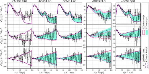
The power spectra monopole (ℓ = 0), quadrupole (ℓ = 2), and hexadecapole (ℓ = 4) for the BOSS/eBOSS data and the corresponding EZmock catalogues are shown in Figs 11 and 12, for NGC and SGC respectively, with the bin size of |$0.01\, h\, {\rm Mpc}^{-1}$|. It can be seen that the differences on the actual number density of tracers between the complete and realistic mocks (see Section 3.1) result in significant biases of the power spectrum amplitude, especially for the monopole of LRGs, which are further enhanced visually due to the small errors. This is because the isotropic number density evaluations are incorrect for the realistic mocks, resulting in biased normalization factors (see Eq.(47)). Nevertheless, this effect does not alter significantly covariance matrices estimations, provided a constant rescaling (see Section A for details).
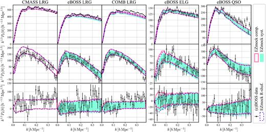
Power spectrum multipoles of the BOSS/eBOSS data and the corresponding EZmock catalogues in NGC. The solid/dashed envelopes and shadowed areas indicate the 1 σ regions evaluated from 1000 mock realizations. The error bars for the CMASS LRG sample are obtained from the complete EZmock catalogues, while for the other tracers they are taken from the realistic mocks with systematics.
Power spectrum multipoles of the BOSS/eBOSS data and the corresponding EZmock catalogues in SGC. The solid/dashed envelopes and shadowed areas indicate the 1 σ regions evaluated from 1000 mock realizations. The error bars for the CMASS LRG sample are obtained from the complete EZmock catalogues, while for the other tracers they are taken from the realistic mocks with systematics.
Apart from the discrepancies on the broad-band amplitude, observational systematics and the ‘shuffled’ random catalogue affects mainly power spectra quadrupole and hexadecapole at |$k \lesssim 0.1\, h\, {\rm Mpc}^{-1}$|. In general, the measurements from the observational data and mocks are in good agreement. Nevertheless, deviations over 1 σ are seen in the power spectra monopole, at |$k \gtrsim 0.25\, h\, {\rm Mpc}^{-1}$| for the eBOSS QSO sample, and |$k \gtrsim 0.15\, h\, {\rm Mpc}^{-1}$| for the combined LRG sample. Since only the eBOSS QSO SGC data is used for the calibration of EZmock QSO catalogues at |$k \gtrsim 0.24\, h\, {\rm Mpc}^{-1}$|, it turns out that the data from a single Galactic cap is not enough for optimal EZmock calibrations at large k.
For the joint CMASS and eBOSS LRG sample, there is an additional mismatch at high k, this may be due to the fact that small scale cross correlations between the BOSS and eBOSS LRGs are not precisely modelled in EZmock catalogues. Since the mocks for the two samples are calibrated separately, their cross correlations are only taken into account through the common dark matter density fields. However, both the inaccuracy of ZA on small scales, and the relatively low resolution of the EZmock density fields (|$\sim 5\, h^{-1}\, {\rm Mpc}$|) prevent precise reproduction of the cross correlations in Fourier space. Similar effects on the cross power spectra between different types of tracers are also observed in Section 4.2. We leave a thorough investigation of this issue to a future study.
Furthermore, in Fig. 12 we observe some oscillatory patterns in the power spectrum quadrupole and hexadecapole for eBOSS ELGs. They are less significant if placing the catalogues into a large box for FFT, see de Mattia et al. (2021), where a box size of 4 |$h^{-1}\, {\rm Gpc}$| is used. This effect may also be suppressed by the multipole estimations with the regression method (Wilson 2016), but a detailed investigation is outside the scope of this paper.
Finally, we plot the correlation matrices of the power spectrum multipoles for different tracers in Fig. 13, with the same definitions as in equations (42) and (43), but the data vectors are replaced by power spectrum multipoles. The impacts of observational systematics and random catalogue generation scheme on the correlation matrices appear to be smaller in Fourier space, compared to the results for 2PCF multipoles.
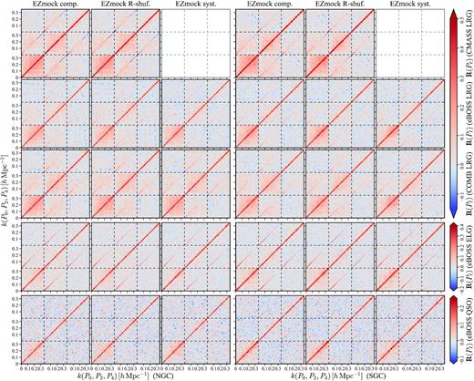
Correlation matrices of power spectrum multipoles obtained from 1000 EZmock realizations.
3.3.2 Bispectrum
The bispectrum is a function of three Fourier space vectors – |$\boldsymbol{k}_1$|, |$\boldsymbol{k}_2$|, and |$\boldsymbol{k}_3$| – that form a triangle. For simplicity we consider only bispectrum monopole for a special configuration of the triangle: two sides are fixed (|$k_1 = 0.1 \pm 0.01\, h\, {\rm Mpc}^{-1}$| and |$k_2 = 0.05 \pm 0.01\, h\, {\rm Mpc}^{-1}$|), and their intersection angle θ12 is varied from 0 to π. The lengths of the sides are chosen to be close to the BAO scale. We use the bispec17 code to compute bispectra, with the grid size of 5123 for the density fields of all tracers.
Apart from the discrepancies on the amplitude due to the approximation of isotropic number densities (see Section A), the agreement between the bispectra of the observational data and EZmock catalogues are again reasonably well, as shown in Fig. 14. For the configuration of the Fourier space triangle we choose, the bispectra are not sensitive to observational systematics and the random catalogue generation method. This ensures that the covariance matrices estimated using EZmock catalogues for the two-point clustering statistics are robust (Baumgarten & Chuang 2018).
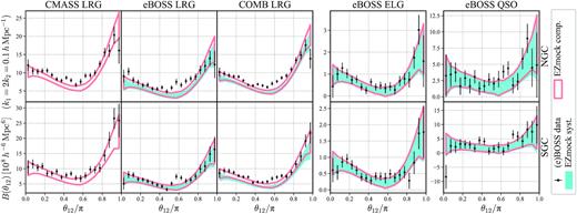
Bispectra of the BOSS/eBOSS data and the corresponding EZmock catalogues, for the two Galactic caps. The solid envelopes and shadowed areas indicate the 1 σ regions evaluated from 1000 mock realizations. The error bars for the CMASS LRG sample are obtained from the complete EZmock catalogues, while for the other tracers they are taken from the realistic mocks with systematics.
3.4 Evolution of clustering
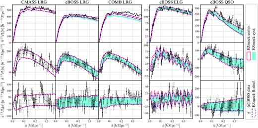
The redshift evolution of EZmock catalogues are modelled by combining snapshots calibrated at several different redshifts (see Section 2.3.5). To validate this scheme, we measure the 2PCF and power spectrum multipoles of the BOSS/eBOSS data and 500 realizations of the corresponding EZmock catalogues in three different redshift bins (apart from CMASS LRGs, for which only two bins are used, due to the low number of galaxies at high redshift). The bins are chosen to contain sufficient data for clustering measurements, as well as close number of tracers in each bin. Besides, we allow overlapping between two adjacent redshift bins. In practice, the redshift bins for the examination of the evolution of EZmock clustering are listed in Table 6. The combined clustering measurements from both Galactic caps are shown in Fig. 15.
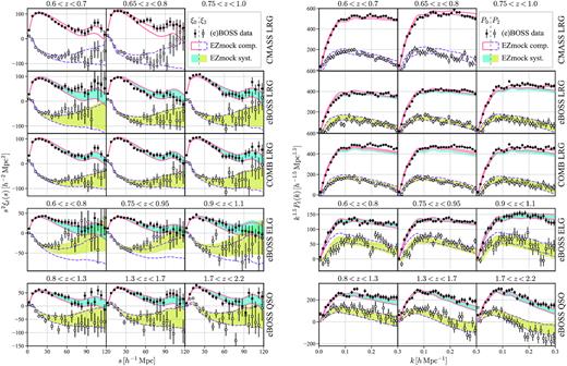
2PCF and power spectrum multipoles of the BOSS/eBOSS data and the corresponding EZmock catalogues in different redshift bins. Measurements from the two Galactic caps are combined. The solid/dashed envelopes and shadowed areas indicate the 1 σ regions evaluated from 500 mock realizations. The error bars for the CMASS LRG sample are obtained from the complete EZmock catalogues, while for the other tracers they are taken from the realistic mocks with systematics.
Redshift bins for the validation of cosmic evolution of EZmock clustering statistics for different tracers.
| bin 1 | bin 2 | bin 3 | |
|---|---|---|---|
| CMASS LRG | 0.6 < z < 0.65 | 0.65 < z < 0.8 | – |
| eBOSS LRG | 0.6 < z < 0.65 | 0.65 < z < 0.8 | 0.75 < z < 1.0 |
| COMB LRG | 0.6 < z < 0.65 | 0.65 < z < 0.8 | 0.75 < z < 1.0 |
| eBOSS ELG | 0.6 < z < 0.8 | 0.75 < z < 0.95 | 0.9 < z < 1.1 |
| eBOSS QSO | 0.8 < z < 1.3 | 1.3 < z < 1.7 | 1.7 < z < 2.2 |
For both configuration space and Fourier space measurements, there is a general trend that the amplitudes are larger at higher redshifts. This is because with the same target selection criteria, objects at higher redshift are more luminous, thus having typically higher biases. This selection effect plays a more important role than structure growth. With the density fields and bias models constructed at different redshifts, EZmock catalogues are able to reproduce both effects. Fig. 15 shows that the cosmic evolution of the clustering statistics of the observational data and EZmock catalogues are generally in good agreements.
3.5 Normality check
The histogram of the chi-squared values for the 2PCF and power spectrum multipoles of all the single mock realizations are shown in Fig. 16. In particular, the monopole, quadrupole, and hexadecapole measurements are all included, for both configuration and Fourier spaces, with the s and k ranges being |$[20, 200]\, h^{-1}\, {\rm Mpc}$| and |$[0.03, 0.25]\, h\, {\rm Mpc}^{-1}$|, respectively. We then compute the probability density function of the chi-squared distribution, with the degrees of freedom being 108 and 66, which are the number of bins for the 2PCF and power spectrum multipole measurements, respectively. Fig. 16 shows that the distributions of the chi-squared measured from the mocks follow almost perfectly the analytical probability distribution. Therefore, the variances of the clustering measurements from the mocks are well consistent with Gaussian random variables.
![The distribution of the chi-squared (equation (50)) for the clustering measurements of 1000 individual EZmock realizations, with respect to the mean results from all the mocks, for 2PCF and power spectrum multipoles (including monopole, quadrupole, and hexadecapole). The ranges of the clustering measurements are $s \in [20, 200]\, h^{-1}\, {\rm Mpc}$ and $k \in [0.03, 0.25]\, h\, {\rm Mpc}^{-1}$, respectively. The solid and dashed lines show the probability density function of the chi-squared distribution, with the degrees of freedom being the number of bins for the corresponding clustering statistics (108 for 2PCF multipoles, and 66 for power spectrum multipoles). Arrows indicate the chi-squared measured with the BOSS/eBOSS data and the mean of the associate mocks.](https://oup.silverchair-cdn.com/oup/backfile/Content_public/Journal/mnras/503/1/10.1093_mnras_stab510/1/m_stab510fig16.jpeg?Expires=1750320684&Signature=IZbleF-MHxRnOLDV5jHXpVAIRuQL~gyyymMqA-hIL1EUr1Hefku1-Zitkb6Qwlcxxod3Vfbb6p7g373QIfIdq1mnMTmDdpiAYAEBPUQEaPZqRRdn83xX6U-KSsTAaGZD~rIPLpytPo7STyZvEKO~C~6sg05Ssmgsg0dEegC86ZHRkaKEvuOTHh8g5USB-N67nBuUxvrhlpjOM5c6MzmYVf~GRoMGcwaLxt9Hfpx5~HHbj32SkOp-U3Mf2maR1QV95yQnt9Hn9cM4HrcGGkFqQ-EnRQ2xUgMWqd30rqVewcnl0WoxvrXLgC2bOAIr2aaTmRtUW043SC4oY28JM0dUAw__&Key-Pair-Id=APKAIE5G5CRDK6RD3PGA)
The distribution of the chi-squared (equation (50)) for the clustering measurements of 1000 individual EZmock realizations, with respect to the mean results from all the mocks, for 2PCF and power spectrum multipoles (including monopole, quadrupole, and hexadecapole). The ranges of the clustering measurements are |$s \in [20, 200]\, h^{-1}\, {\rm Mpc}$| and |$k \in [0.03, 0.25]\, h\, {\rm Mpc}^{-1}$|, respectively. The solid and dashed lines show the probability density function of the chi-squared distribution, with the degrees of freedom being the number of bins for the corresponding clustering statistics (108 for 2PCF multipoles, and 66 for power spectrum multipoles). Arrows indicate the chi-squared measured with the BOSS/eBOSS data and the mean of the associate mocks.
In order to examine the statistical consistency between the BOSS/eBOSS data and EZmock catalogues, we further compute the chi-squared value of the clustering statistics of the observational data, with respect to both the complete and realistic EZmock catalogues, and the results are marked by arrows in Fig. 16. It shows that the realistic mocks are always in better agreements with the observational data in configuration space, compared to the results from the complete mocks. Indeed, the ELG data and mocks are only consistent with observational systematics applied, and with the ‘shuffled’ random catalogue. In general, it is possible to regard the observational data as one particular realization of the statistical ensemble of the realistic mocks, even with the mismatch of the power spectra amplitudes due to the number density evaluation (see Appendix A). It is however less representative for the joint CMASS and eBOSS LRG sample, for which the cross correlations between the two data sets may not be well modelled by EZmock catalogues.
4 CROSS CORRELATIONS
The overlapping volumes between different types of eBOSS tracers – LRGs, ELGs, and QSOs – are sufficient for large-scale clustering measurements, which permits multi-tracer analysis with cross correlations. To have reliable estimations on the covariance matrices for cross clustering measurements, for each of the EZmock realization, all tracers are constructed using the same initial conditions, and applied the same geometric transformation for the light-cone catalogue creation, to ensure the same underlying dark matter density field. Thus, though the mocks for different types of tracers are calibrated separately, their clustering statistics are correlated through the dark matter field. In this section, we investigate the relationship between different tracers, including their cross clustering statistics.
4.1 Spatial relationship
As the EZmock catalogues for different types of tracers share the density field, we first examine their spatial distributions, and compare with the dark matter density field from ZA. In practice, EZmock catalogues for different tracers are populated at different redshifts (see Table 2). Therefore, their dark matter density fields are not identical, but linked through dynamical evolutions. For a direct comparison of tracer distributions, we evaluate the dark matter density field at z = 0.9, and interpolate or extrapolate the EZmock parameters for different eBOSS tracers all at this redshift (see Section 2.5) to construct mock catalogues with exactly the same dark matter distribution.
Fig. 17 shows the projected dark matter density field, as well as the overdensity distribution of different tracers in the same comoving volume. In particular, the overdensities are defined as |$\delta _{\rm t} = \rho _{\rm t} / \bar{\rho }_{\rm t} - 1$|, where ρt indicates the number density of tracers, including dark matter particles, and |$\bar{\rho }_{\rm t}$| denotes the mean density in the full comoving volume. Moreover, the density fields are all calculated using the CIC particle assignment scheme. It can be seen clearly that the large-scale distributions of eBOSS tracers are all in good agreements with the dark matter density field.
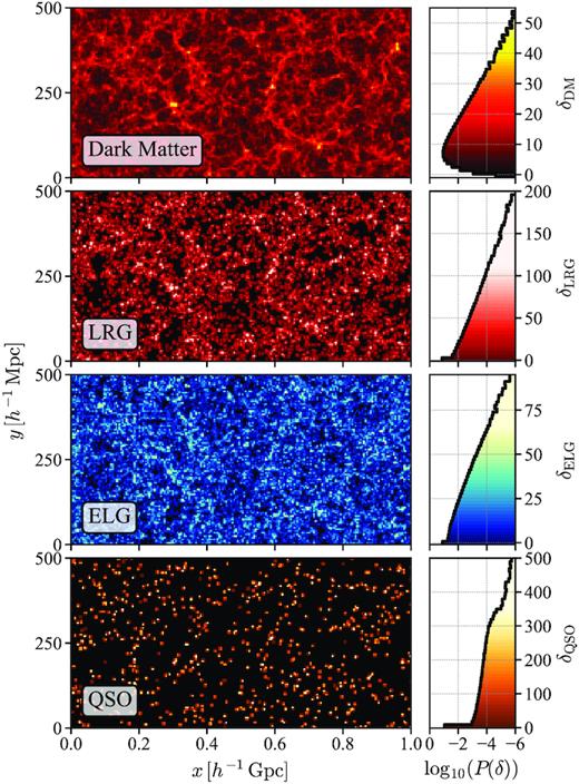
Projected overdensity field for different tracers in a |$2000 \times 500 \times 50\, h^{-3}\, {\rm Mpc}^3$| sub-volume of an EZmock box constructed at z = 0.9 (left panel), and the probability distribution function of the tracer densities in the full box (right panel).
Futhermore, the LRG distribution follows closely that of dark matter, while for ELGs the distribution is more diffused, indicating a lower galaxy bias. Thus, the galaxy distributions in EZmock catalogues are consistent with the mass and environment relationship between passive and star-forming galaxies from observations and simulations (see e.g. Peng et al. 2010; Gonzalez-Perez et al. 2020). The overdensity of QSOs appear to be even higher than that of LRGs, but this is mainly due to their low averaged number density. Indeed, the QSO overdensity field does not always match the dark matter distribution, and the densities are generally too low to reveal cosmic web structures. Therefore, the QSO distribution may not be ideal for estimating the density or gravitational field. Consequently, the BAO reconstruction technique (Eisenstein et al. 2007) may not work well for QSOs.
In order to illustrate the spatial distribution of different types of tracers in the full EZmock light-cone catalogues, we further compare the ‘side view’ of tracer distributions from the eBOSS data and one realistic EZmock realization in a small angular region (10° × 1°), and the plot is shown in Fig. 18. In particular, the upper panel shows the tracer distribution in the full eBOSS redshift range, while the lower panel presents a common redshift range (0.8 < z < 0.9) for all tracers. Statistically there are no obvious differences between the tracer distributions of the data and EZmock realization, and similar filamentary and void patterns can be seen in both catalogues. Again, the ELG distribution is more diffused. But thanks to their high number density, ELGs can be used as references for comparing the distributions of tracers in the shared volume. The lower panel of Fig. 18 reveals tight links between different tracers: most of the LRGs and QSOs reside with ELGs, and there are typically no tracers inside voids of the ELG distributions.

Projected distribution of tracers from the eBOSS DR16 data (right) and one realization of the associated realistic EZmock catalogues with observational systematics (left), in a 10° × 1° region of the sky, with the right ascension between 150° and 160°, and declination between 29° and 30°. The lookback time is evaluated in the flat ΛCDM cosmology with Ωm = 0.31.
4.2 Cross clustering measurements
To quantify the cross correlation between different tracers in the BOSS/eBOSS data and the corresponding EZmock catalogues, we present in this section the cross clustering measurements between different tracers, in both configuration and Fourier space. Since there are not many LRGs and QSOs in a common volume, we consider only the LRG–ELG and ELG–QSO cross correlations. Furthermore, we use the full catalogues for the cross correlation measurements, rather than taking only tracers in the shared volumes.
The cross correlation function and cross power spectrum can be decomposed with Legendre polynomials as well, to obtain the multipole measurements. The formulae are similar to those of the auto correlations, i.e. equations (41) and (48). As the results, the cross clustering multipoles between different BOSS/eBOSS samples and the associated EZmock catalogues are shown in Fig. 19.
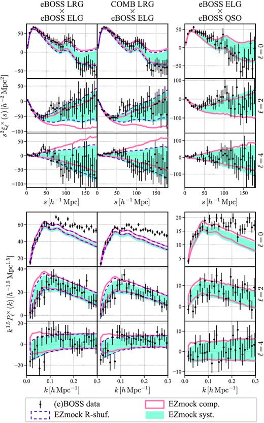
The cross clustering measurements of the BOSS/eBOSS data and the corresponding EZmock catalogues. Results from the two Galactic caps are combined. The solid/dashed envelopes and shadowed areas indicate the 1 σ regions evaluated from 1000 mock realizations.
In general, all the configuration space cross correlation measured from the mocks are in good agreements with those of the observational data, especially for the results computed with the ‘shuffled’ random catalogues. However, for the cross power spectrum multipoles, apart from the discrepancies on the normalizations for the realistic mocks (see Section A), there are also significant mismatches between the data and mocks at high k. As has been discussed in Section 3.3, the small scale cross correlations between different tracers may not be modelled correctly in the EZmock catalogues, by performing the EZmock calibrations separately for different types of tracers. In reality, different tracers may reside in the same galaxy cluster, and are strongly linked with each other. However, this effect are not considered for the EZmock catalogues, in which different tracers are populated in the density field independently. Thus, the cross clustering statistics of the EZmock tracers should be underestimated on small scales. To correct for this effect, further small-scale connections between different tracers should be included (see Alam et al. 2020b, for a multi-tracer HOD approach), and we leave the detailed studies for EZmock catalogues to a future paper.
Though the observational systematics affect the auto correlations of ELGs dramatically, We do not see significant difference comparing the cross-clustering measurements from the realistic mocks with those from complete mocks. The ‘shuffled’ random catalogues are used to compute these measurements. This is because the observational systematics for different tracers are only through foregrounds, e.g. stellar density or galactic extinction, and are not obvious for the cross clustering measurements. For a thorough analysis of the cross correlation function between LRGs and ELGs, see Wang et al. (2020).
5 CONCLUSIONS
We have described the construction of 1000 realizations of EZmock catalogues, for each type of the eBOSS DR16 tracers for LSS analysis, including LRGs (0.6 < z < 1.0), ELGs (0.6 < z < 1.1), and QSOs (0.8 < z < 2.2), as well as the BOSS DR12 CMASS LRGs in the redshift range 0.6 < z < 1.0 for the joint LRG studies, taking into account the cross correlations between different tracers. To this end, 46,000 realizations of simulation boxes are generated, with the side length of |$5\, h^{-1}\, {\rm Gpc}$|. The final mock catalogues are composed of four redshift slices for CMASS LRGs, five slices for eBOSS LRGs, seven slices for eBOSS ELGs, and seven slices for eBOSS QSOs, to account for cosmic evolution of the clustering statistics and sample selection biases at different redshifts.
These mock catalogues encode effective structure formation and tracer bias models, based on the Zel’dovich approximation, and bias descriptions including both deterministic and stochastic effects. Moreover, various geometrical survey features are applied to the mocks, including survey footprints, veto masks, and radial distributions. In addition, both the photometric and spectroscopic systematic effects of the observational data are migrated to the EZmock catalogues, to have robust estimates of the covariance matrices for BAO and RSD analysis.
The EZmock catalogues have shown good agreements with the observational data, in terms of two- and three-point auto-clustering statistics, as well as two point cross correlations. The consistencies are generally within |$1\, \sigma$| for scales down to a few |$h^{-1}\, {\rm Mpc}$| in configuration space, and up to |$0.3\, h\, {\rm Mpc}^{-1}$| in Fourier space, apart from offsets on the normalizations of power spectra due to the definition of isotropic radial selection functions (see Appendix A), and discrepancies at |$k \gtrsim 0.15\, h\, {\rm Mpc}^{-1}$| for cross correlations in Fourier space. And the covariance matrices obtained from these mock catalogues are used for the BAO and RSD measurements of the LRG samples (Bautista et al. 2021; Gil-Marín et al. 2020), ELG samples (de Mattia et al. 2021; Raichoor et al. 2021; Tamone et al. 2020), and QSO samples (Neveux et al. 2020; Hou et al. 2021) for the final eBOSS analysis, as well as the cross correlation studies with LRGs and ELGs (Wang et al. 2020), and the cosmological constraints (eBOSS Collaboration 2020).
The final EZmock catalogues presented in this paper will be made available to the public.18
ACKNOWLEDGEMENTS
We thank the anonymous referee for the valuable comments and suggestions. CZ, AR, and AT acknowledge support from the SNF grant 200020_175751. AR and JPK acknowledge support from the ERC advanced grant LIDA. AdM acknowledges support from the P2IO LabEx (ANR-10-LABX-0038) in the framework ‘Investissements d’Avenir’ (ANR-11-IDEX-0003-01) managed by the Agence Nationale de la Recherche (ANR, France). AJR is grateful for support from the Ohio State University Center for Cosmology and Particle Physics. RN acknowledges support from ANR-17-CE31-0024-01, NILAC. Authors acknowledge support from the ANR eBOSS project (ANR-16-CE31-0021) of the French National Research Agency. GR acknowledges support from the National Research Foundation of Korea (NRF) through Grants No. 2017R1E1A1A01077508 and No. 2020R1A2C1005655 funded by the Korean Ministry of Education, Science and Technology (MoEST), and from the faculty research fund of Sejong University. SA is supported by the European Research Council through the COSFORM Research Grant (#670193).
The massive production of EZmock catalogues was performed at the National Energy Research Scientific Computing Center (NERSC),20 a U.S. Department of Energy Office of Science User Facility operated under Contract No. DE-AC02-05CH11231. We also made use of the Beiluo cluster at Tsinghua University, and Sciama High Performance Computing cluster supported by the ICG, SEPNet and the University of Portsmouth.
Funding for the Sloan Digital Sky Survey IV has been provided by the Alfred P. Sloan Foundation, the U.S. Department of Energy Office of Science, and the Participating Institutions. SDSS-IV acknowledges support and resources from the Center for High-Performance Computing at the University of Utah. The SDSS web site is www.sdss.org.
SDSS-IV is managed by the Astrophysical Research Consortium for the Participating Institutions of the SDSS Collaboration including the Brazilian Participation Group, the Carnegie Institution for Science, Carnegie Mellon University, the Chilean Participation Group, the French Participation Group, Harvard-Smithsonian Center for Astrophysics, Instituto de Astrofísica de Canarias, The Johns Hopkins University, Kavli Institute for the Physics and Mathematics of the Universe (IPMU) / University of Tokyo, the Korean Participation Group, Lawrence Berkeley National Laboratory, Leibniz Institut für Astrophysik Potsdam (AIP), Max-Planck-Institut für Astronomie (MPIA Heidelberg), Max-Planck-Institut für Astrophysik (MPA Garching), Max-Planck-Institut für Extraterrestrische Physik (MPE), National Astronomical Observatories of China, New Mexico State University, New York University, University of Notre Dame, Observatário Nacional / MCTI, The Ohio State University, Pennsylvania State University, Shanghai Astronomical Observatory, United Kingdom Participation Group, Universidad Nacional Autónoma de México, University of Arizona, University of Colorado Boulder, University of Oxford, University of Portsmouth, University of Utah, University of Virginia, University of Washington, University of Wisconsin, Vanderbilt University, and Yale University.
DATA AVAILABILITY
A python interface for EZmock generating is available at https://github.com/cheng-zhao/pyEZmock. Furthermore, the catalogues described in this paper will be made public19 at https://data.sdss.org/sas/dr16/eboss/lss/catalogs/EZmocks.
Footnotes
The BAO and RSD measurements are available at https://sdss.org/science/final-bao-and-rsd-measurements, and see https://sdss.org/science/cosmology-results-from-eboss for the cosmological results.
See https://skfb.ly/6TPBH and https://skfb.ly/6TPBI for 3D illustrations.
The corresponding 3D illustrations are available at https://skfb.ly/6TRz9
‘Chunks’ are regions in which the plate and fibre assignments are performed independently.
However, for efficiency considerations, we use 5123 grids for the calibration of the EZmock QSO sample. In this case, the Nyquist frequency for the NGC and SGC samples are ∼0.24 and |$0.3\, h\, {\rm Mpc}^{-1}$|, respectively. Consequently, EZmock QSO catalogues in the NGC are only calibrated with the range |$k \in [0.1, 0.24]\, h\, {\rm Mpc}^{-1}$|. While for the rest of the mock samples, the calibrations of the power spectra are all performed with |$k \in [0.1, 0.3]\, h\, {\rm Mpc}^{-1}$|
Before the page is brought online, the catalogues can be obtained on request to the corresponding author.
REFERENCES
APPENDIX A: NORMALIZATION OF FOURIER SPACE CLUSTERING MEASUREMENTS WITH ANGULAR INCOMPLETENESS
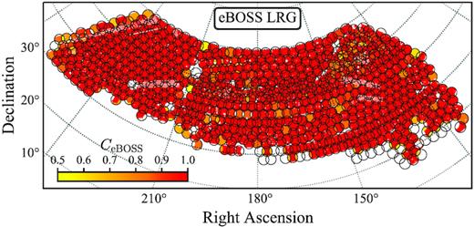
The CeBOSS (fraction of targets without fibres) map of eBOSS LRGs in NGC. Circles indicate the plates for the final LRG data.
To demonstrate this effect, we apply only the incompleteness indicated by the CeBOSS map of the eBOSS LRGs in NGC, to the complete set of EZmock catalogues together with the ‘shuffled’ randoms, and compute the power spectrum multipoles with the |$\tilde{n}_{\rm t}$| estimation described above. The results for these ‘down-sampled’ mocks (denoted by ‘EZmock down.’) are shown in Fig. A2. As expected from the definition of |$\tilde{n}_{\rm t}$|, the amplitude of the power spectrum multipoles from the ‘down-sampled’ mocks are ∼3 per cent lower compared to those of the original catalogues, which is visually particularly obvious for the monopole due to its high amplitude.

The power spectrum multipoles of the re-normalized ‘down-sampled’ mocks with equation (A7) (denoted by ‘EZmock down. renorm.’) are shown in the left-hand panel of Fig. A2, and they are in good agreement with the measurements from the complete mocks. We then apply the nt correction to the realistic EZmock sample, and generate a new set of mocks denoted by ‘EZmock syst. renorm.’. The clustering results are illustrated in the right-hand panel of Fig. A2. One can see that the observational systematics applied to the realistic mocks do not really alter significantly the amplitude of power spectrum multipoles, especially for small wave numbers. However, the discrepancies between the realistic EZmock catalogues and the eBOSS data still exist, as the same re-normalization should be applied to the measurements from the observational data too. Actually, the calibration performed with the complete mocks has already been biased by the inappropriate normalization factor.
To further quantify the impact of this issue on the covariance matrices estimated using EZmock catalogues, we compute the covariance matrices of the power spectrum multipoles with the normalization factors expressed by equations (A3) and (A7) respectively, and the comparisons for the complete and realistic EZmock samples are shown in Fig. A3. As expected, the covariance matrices are generally biased by 6 per cent, which is consistent with the 3 per cent difference on the amplitudes. However, there are also fluctuations on the differences of the covariance matrices, especially for the cross covariances between monopole and the other multipoles. This is because there are separate random catalogues for different realizations, and the re-normalization factors suffer Poisson noises. The fluctuations are more significant for the realistic mocks, since the systematic effects are also different for each random realization. Nevertheless, the diagonal terms are insensitive to the variations of random catalogues, and in general, a rescaling of the covariance matrices works well for correcting the normalization issue.

