


ABSTRACT
O-stars are known to experience a wide range of variability mechanisms originating at both their surface and their near-core regions. Characterization and understanding of this variability and its potential causes are integral for evolutionary calculations. We use a new extensive high-resolution spectroscopic data set to characterize the variability observed in both the spectroscopic and space-based photometric observations of the O+B eclipsing binary HD 165246. We present an updated atmospheric and binary solution for the primary component, involving a high level of microturbulence (|$13_{-1.3}^{+1.0}\,$| km s−1) and a mass of |$M_1=23.7_{-1.4}^{+1.1}$| M⊙, placing it in a sparsely explored region of the Hertzsprung--Russell diagram. Furthermore, we deduce a rotational frequency of |$0.690\pm 0.003\,$|d−1 from the combined photometric and line-profile variability, implying that the primary rotates at 40 per cent of its critical Keplerian rotation rate. We discuss the potential explanations for the overall variability observed in this massive binary, and discuss its evolutionary context.
1 INTRODUCTION
Despite the impact that massive stars (|$M\mathrm{\gt 9\, M_{\odot }}$|) have on the dynamical and chemical evolution of their environment and host galaxy, the physics that determine their evolution are poorly calibrated in theoretical stellar structure and evolutionary models (Kippenhahn, Weigert & Weiss 2012; Langer 2012). In particular, these uncalibrated physics propagate into population synthesis predictions, chemical evolutionary models, and gravitational-wave progenitor predictions. As such, calibrating the input physics that govern massive star evolution is an important goal of astrophysical research. However, due to the diversity of mechanisms that may or may not be active in a given star, calibrating evolutionary models of massive stars can be difficult.
Massive stars exhibit a multitude of phenomena, including (in some cases extreme) wind mass-loss (e.g. Vink et al. 2011; Sander, Vink & Hamann 2019), rapid rotation (e.g. Maeder 2009; Ekström et al. 2012; de Mink et al. 2013; Abdul-Masih et al. 2019), magnetic fields (e.g. Wade et al. 2016; Buysschaert et al. 2017), as well as pulsations (e.g. Aerts, Christensen-Dalsgaard & Kurtz 2010; Handler 2013; Bowman 2020). Additionally, massive O- and B-stars are observed to have a high binary or multiplicity fraction (Kiminki & Kobulnicky 2012; Sana et al. 2012, 2013, 2014; Aldoretta et al. 2015). Large-scale spectroscopic surveys have attempted to populate the upper main-sequence (MS) region of the Hertzsprung–Russell diagram (HRD) in order to characterize the variability there, but face the challenge of disentangling multiple sources of variability (Godart et al. 2017; Simón-Díaz et al. 2017; Burssens et al. 2020). All of these variability mechanisms manifest spectroscopically and photometrically, with their observable effects being useful in constraining the physics responsible for them.
Stars with initial masses between approximately 8 and 25 M⊙, and between 3 and 9 M⊙ have been observed to pulsate in coherent pressure (p) and gravity (g) modes (Aerts et al. 2010) excited by the κ-mechanism (Pamyatnykh 1999), with their dominant restoring forces being the pressure force and the buoyancy force, respectively. Historically, these pulsators were difficult to study from the ground, given the periods involved, however, long time-base, high duty-cycle space-based missions have revealed some of these massive pulsators to be multi-periodic hybrid pulsators (De Cat et al. 2004; Briquet et al. 2007; Daszyńska-Daszkiewicz & Walczak 2010; Szewczuk & Daszyńska-Daszkiewicz 2017; Burssens et al. 2019). In addition to coherent pulsations excited via the κ-mechanism, OB stars are also observed to exhibit internal gravity waves (IGWs; Aerts & Rogers 2015; Aerts, Van Reeth & Tkachenko 2017; Bowman et al. 2019a,b), which are stochastically excited travelling buoyancy waves generated at the interface of the convective core and radiative envelope. Irrespective of the excitation mechanism, these waves cause both spectroscopic and photometric variability in observations (see e.g. Bowman et al. 2020). Additionally, the photometric signal associated with IGWs has been independently reproduced via both 2D (Ratnasingam, Edelmann & Rogers (Horst et al. 2020; Ratnasingam, Edelmann & Rogers 2020) and 3D hydrodynamical simulations (Edelmann et al. 2019).
Whenever active, any of these mechanisms can substantially impact the evolution of a star and its resulting end product. To this end, characterization of the signals present in observations of massive stars is required before they can unambiguously be attributed to some given mechanism(s). As such, massive stars in eclipsing binaries represent some of the best opportunities to achieve this goal, as they provide model-independent estimates of fundamental stellar parameters such as mass and radius. However, the currently-known sample of massive eclipsing binaries with data sets that allow for such precise parameter determination is limited (Torres, Andersen & Giménez 2010; Bonanos et al. 2011; Koumpia & Bonanos 2012; Lohr et al. 2018; Mahy et al. 2020a,b). Even more so, there are fewer systems for which there exist extensive photometric and spectroscopic data sets to characterize the variety of variability.
In this paper, we investigate and characterize the intrinsic variability in the massive detached eclipsing O+B binary HD 165246. To do this, we utilize an extensive spectroscopic data set combined with high-precision space photometry. In Section 3, we determine an updated binary solution, and fundamental parameters for the system. Furthermore, in Section 3.3, we investigate the photometric variability present in the residual light curve after subtraction of the binary model. In Section 4, we introduce and analyse the new spectroscopic data set. Finally, in Section 5, we discuss the potential mechanisms behind the observed variability and briefly discuss the evolutionary context of the system, and present our conclusions in Section 6.
2 THE TARGET HD 165246
HD 165246 (V = 7.6, O8V) has been the focus of several dedicated studies and has been included as part of a larger sample in some spectroscopic surveys of massive stars. Mayer, Harmanec & Pavlovski (2013) made use of 13 FEROS spectra and 617 ASAS3 V-band observations to derive an initial orbital solution for this system, improving on the linear ephemeris deduced by Otero (2007). Mayer et al. (2013) determined a projected rotational velocity of vsin i = 242.6 ± 2.7 km s−1, without including micro- or macroturbulence. In their analysis, Mayer et al. (2013) assumed a mass for the primary of M1 = 21.5 M⊙, obtained by comparing the spectroscopic parameters to theoretical models by Martins, Schaerer & Hillier (2005). From this, the authors determine a full spectroscopic orbital solution via disentangling, enforcing a mass ratio of q = 0.175 as a starting point. They obtained |$T_{\rm eff,1}=33\, 300\pm 400$| and |$T_{\rm eff,2}=15\, 800\pm 700$| K. Furthermore, Mayer et al. (2013) claimed that while the derived primary radius is typical for an O8V star, the solution for the secondary revealed a smaller radius than predicted for its mass. From their solution, Mayer et al. (2013) determined an age of τ = 3.3 ± 0.2 Myr via comparison with rotating theoretical evolutionary tracks (Brott et al. 2011).
Using SAM/NACO measurements obtained with the VLTI, Sana et al. (2014) detected a close bright (ΔHmag = 2.36) companion to the inner binary at a separation of ρ = 30 ± 16 mas, and confirmed the presence of a bright companion (ΔHmag = 3.36) at a separation of ρ = 1.93 ± 0.04 arcsec that was originally detected by Mason et al. (1998). Additionally, Sana et al. (2014) detected two fainter companions (ΔHmag > 5) at separations larger than 6.5 arcsec. Including the two distant fainter companions, HD 165246 is a sextuple system with the 4.6-d O+B eclipsing binary. Without further interferometric observations, additional components interior to the companion at 30 mas cannot be ruled out.
After the failure of a second reaction wheel in 2013, the Kepler satellite was re-purposed as the K2 mission, which scanned the ecliptic in 90-d-long pointings (Howell et al. 2014). Owing to the densely crowded field in K2 Campaign 9, Johnston et al. (2017) extracted an ∼30-d light curve using a custom aperture mask, remarking that the mildly saturated pixels, systematics, and thruster firings rendered the remaining ∼60-d segment of the light curve of too poor quality for science. Assuming a circular orbit, and adopting the mass ratio and primary effective temperature reported by Mayer et al. (2013), Johnston et al. (2017) determined an updated binary model. Investigation of the residuals after subtraction of the optimized binary model revealed multiperiodic variability on time-scales between several hours and a few days. Additionally, high-order harmonics of the orbital frequency as well as a harmonic series whose base frequency is consistent with the rotational frequency of the primary were observed. However, the orbital harmonics may have originated from the assumed circular orbit, which can be mitigated with a larger spectroscopic data set. The authors also note the possibility of Doppler beaming being present, but relegate investigation to future work.
From their binary model, Johnston et al. (2017) estimated 18 per cent contaminating light in the light curve, which is within the 7–43 per cent third light contribution estimated from the magnitude contrasts for the other members of the sextuple system (Sana et al. 2014). This estimate depends on the primary effective temperature and mass ratio adopted from Mayer et al. (2013), and as such is subject to change. Finally, Johnston et al. (2017) concluded that the variability signal likely originates from the primary, but suggest that further follow-up is required for unambiguous characterization.
3 PHOTOMETRIC ANALYSIS
The process of optimizing the binary and atmospheric solutions is an iterative one, with the binary model relying on information determined from an atmospheric solution and vice versa. Hence, we start with an atmospheric solution, then build a binary model, and repeat the atmospheric modelling with the updated information from the binary model. This process is repeated until both solutions no longer change within the output uncertainties. For clarity, we describe the binary and atmospheric processes separately.
3.1 K2 photometry
Due to the brightness of HD 165246, the K2 pixels saturate during the 30-min-cadence mode observations. Additionally, HD 165246 lies in a crowded field towards the galactic centre of the Milky Way and shows potentially contaminating sources in the surrounding pixels. To address this, Johnston et al. (2017) built a custom pixel mask that only included the saturated columns and extracted a custom light curve (hereafter lc-a). Due to thruster firings and the saturated and CCD-bleed columns, however, Johnston et al. (2017) only recovered an ∼29.9 d light curve that was of high enough quality for scientific analysis.
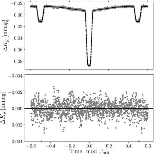
Johnston et al. (2017) concluded that although they identified significant periodicities consistent with both p- and g-mode oscillations, due to the limited time-base of their light curve and lack of an independent means of identifying the origin of the oscillations in combination with the presence of contaminating objects in the pixel image, interpretation of the signal was limited. To increase the frequency resolution of the light curve, we extract a new, longer time-base light curve constructed via the halo photometry method (hereafter lc-b). In this method, the scattered light from bright targets across the entire pixel image are collected, with relative weights given to each pixel to scale their contribution to the resulting light curve (White et al. 2017; Pope et al. 2019). Whereas lc-a only has a time-base TA ∼ 29.9 d, lc-b has a time-base of TB ∼ 71.3 d, improving the formal frequency resolution from dfA = 1/TA = 0.034 d−1 for lc-a to dfB = 1/TB = 0.014 d−1 for lc-b. However, due to the weighting scheme used by the halo photometry method, all additional sources present in the mask contribute contaminating signal to the light curve. This not only increases the overall ‘third light’, but also potentially adds new variability with an unknown amplitude from a contaminating source. Since we know neither whether these separate sources are in fact variable, nor with what amplitudes they may be varying, it is difficult to determine their individual contributions to lc-b. A comparison of the light curves extracted by Johnston et al. (2017) (grey) and in this work (black) is shown in Fig. 1. The clear difference in eclipse depth is caused by the large increase in contaminating light included in lc-b.

Custom extracted K2 light curve of HD 165246 from Johnston et al. (2017) (lc-a; grey) and halo photometry light curve of HD 165246 (lc-b; black).
3.2 Updated binary model
This section discusses the setup for modelling lc-a. The modelling of lc-b is carried out differently, as discussed below. Our initial binary model is based on the solution of Johnston et al. (2017), but incorporates the updated eccentricity and argument of periastron (see Section 4.1.1), as well as the primary effective temperature (see Section 4.3). We optimize our binary model using a Bayesian Markov chain Monte Carlo (MCMC) numeric sampling code emcee developed by Foreman-Mackey et al. (2013) and draw uncertainties from the posteriors, as was done by Johnston et al. (2017). We calculate the binary model using the ellc code (Maxted 2016). In a recent head-to-head comparison, ellc, PHOEBE 1 (Prsa et al. 2011), PHOEBE2 (Prša et al. 2016), JKTEBOP (Southworth 2013), and WD2007 (Van Hamme & Wilson 2007) were all shown to agree to ∼0.4 per cent in the reported fundamental parameters of of the eclipsing binary AI Phe (Maxted et al. 2020). While the authors point out that formal uncertainties are often underestimated when drawn directly from a co-variance matrix, the consistency of their solutions demonstrate that we should not expect any systematic offsets in our solution compared to that of Johnston et al. (2017) based on the use of a different code. In order to incorporate the spectroscopic information, we impose Gaussian priors on the eccentricity |$e\sim \mathcal {N}\left(0.029,0.003\right)$|, the argument of periastron, |$\omega _0\sim \mathcal {N}\left(1.63,0.09\right)$| rad, the semi-amplitude of the primary |$K_1\sim \mathcal {N}\left(53.0,0.2\right)$| km s−1, the effective temperature of the primary |$T_{\rm eff,1}\sim \mathcal {N}\left(36\,150, 600\right)$| K, and the projected rotational velocity of the primary |$v_1 \sin i\sim \mathcal {N}\left(268, 25\right)$| km s−1. The remaining parameters listed in Table 1 are given uniform priors. We allow the mass ratio, q = M2/M1 = K1/K2, to vary freely so as to not bias the fitting result. Similarly, we allow the third light, l3, to vary freely as well.
Estimated parameters returned from the MCMC-optimized ellc binary model.
| Parameter | Unit | Estimate |
|---|---|---|
| R1/a | – | |$0.208 ^{+0.001}_{-0.001}$| |
| R2/a | – | |$0.069^{+0.001}_{-0.002}$| |
| a | R⊙ | |$35.3^{+0.6}_{-0.7}$| |
| Sb | – | |$0.217^{+0.004}_{-0.006}$| |
| q | – | |$0.16^{+0.02}_{-0.02}$| |
| i | ° | |$84.0^{+0.1}_{-0.1}$| |
| Porb | d | |$4.592\,70^{+0.000\,01}_{-0.000\,01}$| |
| t0 | d | |$2457\,215.4108^{+0.0004}_{-0.0005}$| |
| fc | – | |$0.0032^{+0.0008}_{-0.0008}$| |
| fs | – | |$0.1656^{+0.0009}_{-0.0007}$| |
| F1 | – | |$3.1^{+0.2}_{-0.1}$| |
| A1 | – | |$0.30^{+0.1}_{-0.2}$| |
| B1 | – | |$2.0^{+0.5}_{-0.5}$| |
| l3, a | per cent | |$26^{+2}_{-1}$| |
| l3, b | per cent | |$67^{+1}_{-1}$| |
| |$T_{\rm eff,1}^{\it a}$| | K | |$36\,100^{+200}_{-200}$| |
| |$T_{\rm eff,2}^{\it a}$| | K | |$12\,100^{+600}_{-600}$| |
| Derived parameters | ||
| e | – | |$0.027^{+0.003}_{-0.002}$| |
| ω0 | rad | |$1.55^{+0.01}_{-0.01}$| |
| k | – | |$0.333^{+0.007}_{-0.009}$| |
| (r1 + r2)/a | – | |$0.2766^{+0.002}_{-0.001}$| |
| L2/L1 | – | |$0.0241^{+0.002}_{-0.001}$| |
| M1 | M⊙ | |$23.7^{+1.1}_{-1.4}$| |
| R1 | R⊙ | |$7.3^{+0.3}_{-0.4}$| |
| log g1 | dex | |$4.08^{+0.02}_{-0.04}$| |
| M2 | M⊙ | 3|$.8^{+0.4}_{-0.5}$| |
| R2 | R⊙ | |$2.4^{+0.3}_{-0.1}$| |
| log g2 | dex | |$4.26^{+0.06}_{-0.14}$| |
We refer to Maxted (2016) for the meaning of the symbols. aQuantities only used to calculate limb- and gravity-darkening coefficients.
Instead of directly fitting for the effective temperatures, ellc fits for the surface brightness ratio. To this end, the effective temperature and surface gravities of each component are only used to interpolate values for the limb-darkening and gravity-darkening coefficients in the Kepler passband from the tables published by Claret & Bloemen (2011). As such, we sample the effective temperatures of each component and use the surface gravities computed for each model as inputs to interpolate for the limb- and gravity darkening coefficients. Following the suggestion of Johnston et al. (2017), we include Doppler boosting in our model in order to account for the asymmetric out-of-eclipse photometric variability observed in the residuals. We include both the light curve and radial velocity (RV) measurements in our fitting procedure.
We run 10 000 iterations with 128 individual chains in our MCMC optimization routine, discarding those iterations that occurred before five times the autocorrelation time as burn-in. The parameter estimates and uncertainties listed in Table 1 are calculated as the median and 68.3-percentile highest posterior density (HPD) confidence interval estimates of the marginalized posteriors for each parameter. The derived quantities, such as the masses and radii of each component, are calculated at each iteration and saved along with the other sampled parameters, allowing us to calculate the estimates and uncertainties for these parameters in the same way. The best-fitting model, shown in black in the top panel of Fig. 2, is calculated from the values listed in Table 1. The residuals shown in the bottom panel of Fig. 2 have a root mean square (rms) scatter of 0.89 mmag. We note that the residuals calculated for the same model but without Doppler boosting have an rms scatter of 0.91 mmag, and display a brightening event at Φ ∼ 0.3, which is consistent with the phase when the O-star is accelerating towards the line of sight. Furthermore, we note that a significant peak is present at the orbital frequency in the periodogram of the residuals for the model without beaming included. This peak is not detected in the residuals of the model with beaming included.
Top panel: K2 observations (grey) and the best-fitting model (black) for HD 165246. Bottom panel: residuals (grey) after the removal of the best-fitting model.
Beyond the inclusion of the eccentricity, boosting factor, and updated Teff, 1 in our improved binary model, we find a lower mass ratio compared to that of Mayer et al. (2013). We note that this may be caused by the inclusion of third light in our model. The estimated third light contribution of |$26\substack{+2\\-1}$| per cent is within the estimates of 7–43 per cent expected from the other members of the sextuple system as derived from the K-band magnitude contrasts published by Sana et al. (2014). As a combined result, we calculate that the primary has |$M_1=23.7\substack{+1.1\\-1.4}$| M⊙ with |$R_1=7.3\substack{+0.3\\-0.4}$|R⊙, and the secondary has M2 = 3|$.8\substack{+0.4\\-0.5}$| M⊙ with |$R_2=2.4\substack{+0.3\\-0.1}$|R⊙.
As mentioned previously, the modelling of lc-b is conducted differently to that of lc-a. Since we expect the physical binary model to be the same, but the third light contribution to be different, we fix the model and sample only the third light contribution for lc-b. From this, we find that lc-b has roughly 66 per cent composite contaminating light, which is significantly larger than the range expected from the other members of the sextuple system. This suggests that this light contains rescaled contributions from other stars in the K2 pixel image.
3.3 Photometric variability
We use the residuals of lc-a and lc-b after removal of the optimized binary model (hereafter res-a and res-b, respectively) to calculate a Lomb–Scargle periodogram with the aim of searching for significant periodicities. The periodograms for res-a and res-b are shown in the top and bottom panels of Fig. 3. We subject both res-a and res-b to an iterative pre-whitening process to extract all variability with an amplitude signal-to-noise ratio (S/N) greater than four (i.e. S/N > 4; Breger et al. 1993), where the S/N is calculated over the full range ν ∈[0, 24.5] d−1 up to the Nyquist frequency. Except for one frequency, f14, there is no overlap in the extracted frequency lists for res-a and res-b.
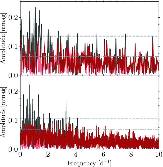
Top panel: Lomb–Scargle periodogram of res-a (black) and its residuals (red). Bottom panel: Lomb–Scargle periodogram of res-b (black) and its residuals (red). Horizontal dashed dark grey and dashed-dotted light grey lines denote four times the white noise level in the residual periodograms after binary model removal and pre-whitening, respectively.
Given the greater than factor of 2 increase in contaminating light between the two light curves, and lack of similarity between the extracted frequency lists from res-a and res-b, we only consider those frequencies extracted from res-a in our subsequent analyses. The lack of overlap in extracted frequencies between the two lists does not imply that the signal is not present in res-b. Rather, given the increase in contaminating light, the signal is simply no longer significant according to our S/N > 4 criterion. We suggest that the frequencies extracted from res-b likely originate in one, or several, of the contaminating stars included in the halo-photometry mask, and not from the components of the HD 165246 system. The frequencies extracted from res-a are given in Table 2. The tabulated frequencies have been filtered for close frequencies occurring within 1.5 times the Rayleigh criterion (Degroote et al. 2009, 2010; Pápics et al. 2012; Bowman 2017).
Iterative pre-whitening results for the residuals of res-a.
| lc-a | ||||
|---|---|---|---|---|
| ID | Frequency | amplitude | S/N | Note |
| (d−1) | (mmag) | |||
| fp, 1 | 0.502 ± 0.004 | 0.15 | 4.61 | fs, 9 |
| fp, 2 | 0.690 ± 0.003 | 0.22 | 6.26 | fs, 15 |
| fp, 3 | 0.992 ± 0.003 | 0.23 | 6.45 | fs, 17 |
| fp, 4 | 1.117 ± 0.003 | 0.23 | 6.55 | – |
| fp, 5 | 1.305 ± 0.004 | 0.15 | 4.59 | 6forb |
| fp, 6 | 1.382 ± 0.003 | 0.21 | 6.20 | 2fp, 3 |
| fp, 7 | 1.502 ± 0.004 | 0.14 | 4.59 | fs, 14 |
| fp, 8 | 1.540 ± 0.003 | 0.18 | 5.22 | – |
| fp, 9 | 2.004 ± 0.003 | 0.16 | 4.92 | – |
| fp, 10 | 2.057 ± 0.004 | 0.15 | 4.68 | 3fp, 3 |
| fp, 11 | 2.165 ± 0.004 | 0.14 | 4.45 | – |
| fp, 12 | 2.755 ± 0.004 | 0.16 | 4.70 | 4fp, 3 |
| fp, 13 | 3.448 ± 0.004 | 0.13 | 4.28 | 5fp, 3 |
| fp, 14 | 4.139 ± 0.004 | 0.14 | 4.68 | 6fp, 3 |
| fp, 15 | 5.529 ± 0.004 | 0.15 | 4.64 | 8f3 |
| fp, 16 | 6.900 ± 0.004 | 0.15 | 4.16 | 10fp, 3 |
| fp, 17 | 7.601 ± 0.004 | 0.13 | 4.55 | 11fp, 3 |
In contrast to Johnston et al. (2017), we identify only one harmonic of the orbital frequency in res-a (fp, 5). This is a consequence of the improved binary model. As indicated in Table 2, fp, 1, fp, 2, fp, 3, and fp, 7 are also extracted in the LPV analysis in Section 4.1.2. Furthermore, we find nine components (1,2,3,4,5,6,8,10,11) of a harmonic series with fp, 2 = 0.690 ± 0.003 d−1 as the base frequency. Extended harmonic series are the result of non-sinusoidal signals in the light curve, such as binarity, rotational modulation, or high-amplitude pulsation. The latter option is excluded as all detected amplitudes are below 1 mmag. To investigate the former option, we phase res-a over fp, 2 = 0.69 in Fig. 4 and find no obvious indication of a blended binary signal. Assuming fp, 2 is the rotation frequency, one expects F1 = fp, 2/forb = 3.17 ± 0.01, which is within 1 − σ of the value for F1 obtained from our binary modelling in Section 3.2, indicating that the rotational interpretation is feasible. Using fp, 2 = frot as well as R1 and i from Table 1 to compute v1sin i yields |$v_1\sin i=253^{+11}_{-14}$| km s−1. This matches well with the value estimated from spectroscopy in Section 4.3. This harmonic rotational signal could be caused by wind variability modulated by the stars rotation (i.e. a clumpy wind), although we do not detect strong wind signatures in the typical diagnostic lines for HD 165246. Nevertheless, the recovery of a significant (S/N > 4) signal at fs, 15 ≃ fp, 2 in the LPVs with a full 2π variation over the line profile also suggests an interpretation of this signal in terms of rotational modulation.
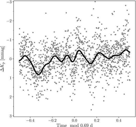
res-a phase folded over fp, 3. Original data in grey, binned data in black.
The Lomb–Scargle periodogram of the pre-whitened residuals of both res-a and res-b are shown in red in the respective panels of Fig. 3. These periodograms showcase stochastic low-frequency variability as found previously for a large sample of CoRoT, K2, and Transiting Exoplanet Survey Satellite (TESS) OB stars (Blomme et al. 2011; Aerts & Rogers 2015; Aerts et al. 2018; Simón-Díaz et al. 2018; Bowman et al. 2019b, a). Such a signal is predicted independently by 3D hydrodynamic simulations carried out by Edelmann et al. (2019) as well as by different 2D hydrodynamic simulations by Horst et al. (2020) and Ratnasingam et al. (2020). All of these simulations concerned single, young stars. However, given the complexity of this multiple system, other physical causes of this excess may be relevant as well. The stochastic variability occurs in both res-a and res-b and is significant according to the S/N > 4 level when the latter is computed from the residual periodogram computed from zero frequency up to the Nyquist frequency (see the dash–dotted horizontal line in Fig. 3). Our argument to consider such a broad range of frequencies to compute the noise level follows Blomme et al. (2011) and Bowman et al. (2020), who have shown that young massive O stars such as the primary component of HD 165246 have significant low-frequency variability up to frequencies of the order of 100 d−1.
4 SPECTROSCOPIC ANALYSIS
We also investigate the presence of line-profile variability in HD 165246 on various time-scales. To do this, we obtained 160 observations between 2017 May 3 and 2019 October 10 with the hermes spectrograph (R = |$85\, 000$|; Raskin et al. 2011) attached to the 1.2-m Mercator telescope at El Observatario Roque de los Muchachos in Santa Cruz de La Palma. As many as 20 consecutive exposures were taken during eight nights in order to achieve a high temporal resolution. The observations have a mean S/N = 85 at 550 nm (ranging from S/N = 63 for the lowest quality observation to S/N = 112 for the highest quality observation), with an average integration time of 1200 s, and are well distributed across the orbit. These observations were subjected to background and bias subtraction, flat fielding, wavelength calibration (ThAr lamp spectrum), and order merging using the local hermes pipeline. The reduced spectra were subsequently normalized via spline fitting.
To maximize the S/N for the spectra, we calculate a least-squares deconvolved (LSD) profile (Donati et al. 1997; Tkachenko et al. 2013). This method involves convolving a series of δ functions of given depths at a given set of wavelengths corresponding to a pre-determined mask to produce an average line profile from the entire spectrum. Thus, the expected increase in S/N is proportional to |$\sqrt{N}$|, where N is the number of spectral lines used in the mask. Furthermore, by allowing for the simultaneous calculation of multiple average profiles, the LSD methodology enables the detection of multiple components in the spectrum. Whereas the spectra of O-stars feature strong He ii lines, the optical spectra of B-type or cooler stars feature strong He i or metal lines, depending on the effective temperature. To this end, the use of different masks allows for the detection of multiple components should they have a significant light contribution.
Following these considerations, we subject all of the available hermes spectra to this method considering two different masks: (i) helium lines between 4900 and 5900 Å, and (ii) metal lines, both of which were constructed from the VALD data base (Kupka et al. 1999). Since hydrogen and helium lines are known to suffer from Stark broadening and the signature of radiation-driven winds (should they be present), these lines are generally avoided in line-profile variability studies. However, in the case of hot rapidly rotating stars, helium lines may be the only lines with sufficient S/N to be considered reliable (Balona, Aerts & Štefl 1999; Rivinius, Baade & Štefl 2003). Fig. 5 shows the average LSD profiles constructed using the helium-line mask (black) and the metal-line mask (grey). The average metal-line profile exhibits a trend in the red wing. Although it is unclear what introduces this ubiquitous trend in the LSD profiles produced with the metal-line mask, it is clear that these profiles are unsuitable for line-profile analysis. The average helium-line profile is well behaved. As such, the remainder of the orbital and line-profile analysis is carried out using the LSD profiles produced with the helium-line mask.
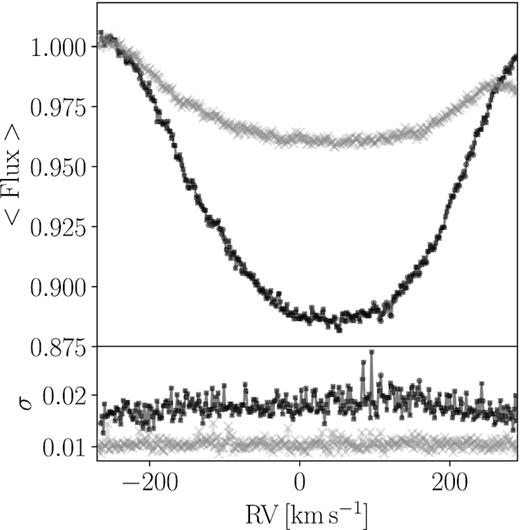
Top panel: mean LSD profile for mask containing only He lines between 4900 and 5900 Å (black) and only metal lines across the whole wavelength range (grey). Bottom panel: standard deviation across LSD profiles.
4.1 Line-profile variability
The overall position and shape of a line profile is the combination of extrinsic and intrinsic broadening effects and perturbations, such as RV shifts due to binarity, broadening due to rotation, micro- or macroturbulence, and stellar pulsations, some of which are variable in time. Thus, studying the line-profile variations (LPVs) over time allows for the investigation of these signals.
The velocity field produced by coherent/stochastic stellar pulsations induces strictly-/quasi-periodic variations in the line-forming regions near the stellar surface. These variations are detectable via time-resolved spectroscopic observations. Whereas pressure waves have a predominantly radial contribution to the line profile (Aerts & De Cat 2003), gravity waves produce predominantly tangential velocity variations in the line profile (De Cat & Aerts 2002). It is worth noting that, although they are expected to be weak in late O dwarfs, line-driven winds of massive stars are thought to be inherently unstable, introducing yet an additional cause of variability into the line-forming region (Puls, Vink & Najarro 2008; Sundqvist et al. 2011). However, the observational consequences of such winds are only important in cases where they are evident in the observations. Moreover, wind variability is stochastic and readily distinguishable from strictly-periodic coherent oscillation modes.
Spectroscopic frequency analysis of coherent pulsation modes employs one of two methods: (i) the moment method (Balona 1986; Aerts, de Pauw & Waelkens 1992; Briquet & Aerts 2003), or (ii) the pixel-by-pixel method (Schrijvers et al. 1997; Mantegazza, Zerbi & Sacchi 2000; Zima 2006; Zima et al. 2006). The moment method involves numerically integrating the moments of the extracted spectral line to describe the variability in terms of the equivalent width (zeroth moment), the centroid velocity (corresponding to RV; 1st moment), profile width (second moment), and profile skewness (third moment). The moment method is most robust for cases where the star is not rapidly rotating (|$v\sin i\lt 50 \, {\rm km \, s^{-1}}$|). There are some notable exceptions, such as for studying rotational variability in rapidly rotating chemically peculiar stars (e.g. Lehmann et al. 2006). However, it can still be useful for identifying periodicities when combined with the pixel-by-pixel method for analysis of rapidly-rotating stars. In contrast to the moment method that relies on the statistical properties of a line profile, the pixel-by-pixel method relies on the phase and amplitude caused by a stellar pulsation mode across the line profile. While the pixel-by-pixel method is more useful in cases where |$v\sin i\gtrsim 50 \, {\rm km \, s^{-1}}$|, it is limited by S/N and is not coupled to the theory of non-radial oscillations as is the case with the moment method. We use the famias software package (Zima 2008) to carry out the LPV analysis, using both the moment and pixel-by-pixel methods.
4.1.1 Orbital variability
The dominant source of variability among the spectra is the RV shift induced by the binary motion. In order to investigate any signal caused by stellar pulsations, we must first effectively model and remove this orbital signal. To do this, we calculate the first moment for all LSD profiles based on the He mask and fit a model to these RV shifts using MCMC, as was done with the eclipse modelling in Section 3.2. We fix the orbital period to Porb = 4.592 70 d and sample the time of periastron passage tpp, the eccentricity e, the argument of periastron ω0, the semi-amplitude of the primary K1, and the systemic velocity γ. We derive estimates and 1σ uncertainties as the median and 68.3 percentile HPD of the marginalized posteriors, which are listed in Table 3. The resulting best fit constructed from these values and the residuals are shown in the top and bottom panels of Fig. 6. The residuals show a peak-to-peak scatter of ∼20 km s−1, indicating the presence of intrinsic variability. Our values for K1, γ, ω0, and e are different from those obtained by Mayer et al. (2013). However, given such a small eccentricity and an argument of periastron near 90°, differing solutions for small data sets, such as that used by Mayer et al. (2013), are not unexpected.
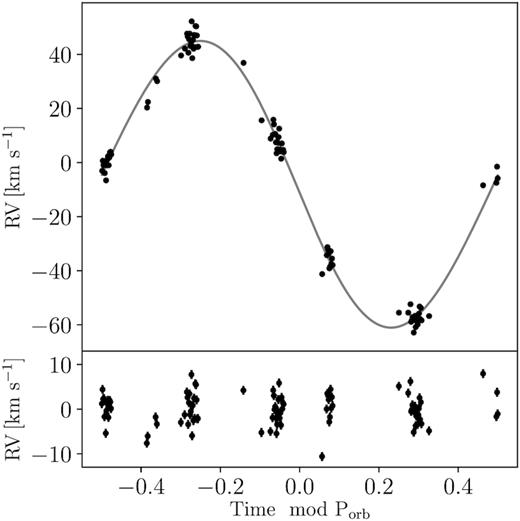
Top panel: observed RVs for HD 165246A in black, the best-fitting orbital solution in grey. Bottom panel: residuals after subtraction of the best-fitting solution. The observed scatter is astrophysical in nature.
Top columns show the HPD estimates and uncertainties for orbital solution, and the bottom columns show the derived values projected distance of the primary to the common centre of mass and the binary mass function, and their uncertainties.
| Parameter | Unit | HPD estimate |
|---|---|---|
| Porb | BJD | 4.592 70 (fixed) |
| tppx | BJD | |$2457\,215.48^{+0.06}_{-0.06}$| |
| e | – | |$0.030^{+0.003}_{-0.003}$| |
| ω0 | rad | |$1.63^{+0.08}_{-0.09}$| |
| K1 | |${\rm km\, s^{-1}}$| | |$53.0^{+0.2}_{-0.2}$| |
| γ | |${\rm km\, s^{-1}}$| | |$-7.9^{+0.1}_{-0.1}$| |
| a1sin i | R⊙ | |$4.81^{+0.01}_{-0.01}$| |
| f(M) | M⊙ | |$0.071^{+0.001}_{-0.001}$| |
We do not detect the presence of the secondary in any of the individual spectra, their LSD profiles, or in the first moment of these profiles. Additionally, we subject the original data set to spectroscopic disentangling using FDBinary (Ilijic et al. 2004; Pavlovski & Hensberge 2005), with a fixed orbital solution according to those values listed in Table 3 and only allow K2 to vary, but are not able to reliably determine a solution.
4.1.2 Intrinsic variability
We remove the orbital motion of the primary from each of the normalized spectra according to the optimized parameters in Table 3. Following this, we calculate new LSD profiles using the helium line mask. These LSD profiles are then used in an LPV analysis, where each LSD profile is assigned a weight according to its S/N. We calculate the zeroth, first, second, and third moments for the data set and subject them to iterative pre-whitening until all periodicities with S/N > 4 are removed from the time-series of these four moments. Table 4 lists the 17 significant frequencies that we identify in the different moments and in the variability across the LSD profiles as found by the so-called velocity pixel-by-pixel method (see Zima 2008). In this method, one searches for variability that occur across the entire LSD profile in velocity space, at a given frequency. In application, we fix the frequency values as found in the photometry or moments and only retain those frequencies for which variability with a significant (S/N > 4) is detected across the LSD profile. We fix the frequencies in order to obtain the highest precision fit results for the amplitude and phase behaviour across the LSD profile, as is common practice in such applications (Zima et al. 2006). We show the periodograms of the moments in Appendix A and the amplitude and phase distributions across the LSDs in Fig. 7. We note that 11 of the frequencies recovered from the frequency analysis of the different moments are newly discovered frequencies, while one is also identified in the photometry, i.e. fs, 9 = fp, 1. The remaining five frequencies recovered via the pixel-by-pixel method are, as expected, also present in either the photometry or spectroscopy.
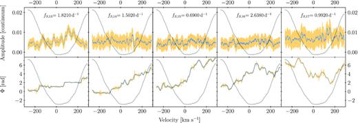
Top panel: amplitude across the line profile. Bottom panel: phase across the line profile. Smoothed data displayed in blue, errors displayed in orange. Line profile overplotted in grey in both panels.
This LPV frequency analysis result is indicative of low- to high-order p- and g-mode pulsational variability. Indeed, the frequencies found previously in rapidly rotating |$\beta \,$|Cep pulsators are markedly higher than those we find for HD 165246 (e.g. Schrijvers, Telting & Aerts 2004; Uytterhoeven et al. 2004, 2005), except for the frequencies fs, 4 and fs, 10. Aside from these two frequencies, all the other frequencies are lower than those of the p modes found in the CoRoT space photometry of the slowly rotating O-type dwarf HD 46202 (Briquet et al. 2011), which is, to date, the |$\beta \,$|Cep star with the highest mass (24 M⊙) determined from asteroseismic modelling.
As expected we find common frequencies among the various moments deduced from the LSD time-series. Matches occur between fs, 2 and fs, 11, fs, 6 and fs, 13, and fs, 8 and fs, 16. Additionally, we note that fs, 9 = fp, 1. Of the five frequencies recovered by the pixel-by-pixel method, three are frequencies from the space photometry and two are from the spectroscopic moments. Of these, we note that fs, 15 = fp, 2 is identified as the rotational frequency. Fig. 7 shows the results of optimizing the amplitude (top row) and phase (bottom row) and their errors, smoothed over a 15 km s−1 window in blue and orange, respectively. Additionally, we plot the average LSD profile in grey. With the exception of fs, 13, the amplitudes across the line profiles are constant within the uncertainties and do not allow us to interpret the results in terms of mode identification. Phase variability as expected for low-amplitude coherent modes can be seen in some of the bottom panels of Fig. 7, particularly for fs, 13. IGWs would result in more chaotic phase variability across the LSD profiles. The phase variability we detect for fs, 14, fs, 16, and fs, 17 has a similar level to that found for some of the lowest amplitude high-degree p modes found in |$\nu \,$|Cen (Schrijvers et al. 2004), |$\lambda \,$|Sco (Uytterhoeven et al. 2004), and |$\kappa \,$|Sco (Uytterhoeven et al. 2005). In Section 3.3, we argued that fp, 2 = fs, 15 can be explained as the rotation frequency of the primary. The full 2π phase variation across the line profile is consistent with this interpretation.
In conclusion, the complex interplay of frequencies, some of which found in both space photometry and high-resolution spectroscopy, is not exceptional (e.g. Cotton et al., submitted, treating the high-mass |$\beta \,$|Cep pulsator |$\beta \,$|Cru). This, along with the frequency regime found for the p modes of the O9V slowly rotating |$\beta \,$|Cep star HD 46202 (Briquet et al. 2011), makes us interpret the frequencies detected in the LSD and in the space photometry of HD 165246 as due to a mixture of coherent low-order p and g modes, along with IGWs, shifted into the gravito-inertial regime by the star’s fast rotation (Aerts, Mathis & Rogers 2019).
4.2 Interpretation as variable macroturbulence
It is well known that rotational broadening alone is not sufficient to explain the shape of line profiles in massive stars (Gray 2005). A microturbulent velocity component, which represents turbulent pressure on spatial scales smaller than the mean-free path of a photon, is added during the atmosphere calculations, and can thus alter the line strength and estimated effective temperature. Furthermore, a macroturbulent velocity component, ξmacro, which represents turbulent pressure on spatial scales larger than the mean-free path of a photon, is required to better reproduce the shapes of massive star line profiles (Howarth et al. 1997; Gray 2005; Aerts et al. 2009; Simón-Díaz & Herrero 2014). The macroturbulent velocity profile can be either anisotropic (with different radial and tangential contributions) or isotropic (with equal radial and tangential contributions). Moreover, while a microturbulent component is considered during the atmospheric calculations, both macroturbulence and rotational broadening are included via convolution to an already computed spectrum, making their contribution to line shape degenerate. Additionally, those stars which undergo other phenomena such as sub-surface convection, spots, and/or stellar pulsations that impact the shape of the line profile and make it asymmetric require further consideration to accurately reproduce the line profile (Aerts et al. 2014).
A non-radial pulsation produces asymmetric deviations from the static line profile that travel through the line profile over the pulsation phase. Thus, the presence of pulsations can directly influence the measurement of observed quantities, such as ξmacro. Aerts et al. (2009) and Aerts & Rogers (2015) demonstrated that the collective contribution of stellar oscillation modes and IGWs, respectively, can explain, at least in part, the observed macroturbulence deduced from the spectral-line properties of massive stars. Aerts et al. (2009, 2014) also caution that determination of vsin i can be complicated by the presence of stellar pulsations that induce asymmetric time-dependent variations in the line profile, a problem made worse when spectra obtained at drastically different pulsation phases are stacked. Furthermore, Aerts et al. (2014) show that the macroturbulence needed to explain purely pulsational broadening can be on the order of or larger than the value of the rotational velocity, and is variable over the pulsation cycle.
As we observe pulsations and a large projected rotational velocity in the O-star primary of HD 165246, it is important that we obtain an independent estimate of vsin i to use as a constraint in the atmospheric modelling. We achieve this by using the iacob-broad tool developed by Simón-Díaz & Herrero (2014) to independently estimate vsin i for the cases considering no macroturbulence, using the first moment of the Fourier transform (FT) and performing goodness-of-fit (GOF) calculations, both allowing for isotropic macroturbulence. We select 10 spectra from our data set, five of which span the range of the entire data set and the other five of which were taken on a single night. This allows us to investigate the stability of the vsin i and ξmacro estimates over different time-scales and at different points along any variability cycle. Given the S/N of our spectra, we use the He ii 4541 line for our calculations. The results of using iacob-broad on the He ii 4541 line are listed in Table 5.
As expected, the estimates of vsin i are systematically higher when ξmacro is fixed at 0 km s−1, yielding vsin i = 268 ± 25 km s−1 compared to vsin iFT = 238 ± 40 and vsin iGOF = 230 ± 46 km s−1. The presence of pulsations in HD 165246, however, complicates the interpretation of this. Aerts et al. (2014) demonstrated that even low-amplitude pulsations can produce either over- or underestimations of vsin i, and hence ξmacro, by the FT method if a simple isotropic model of macroturbulence is used, depending on the pulsation phase of the observed spectrum. This is because a time-independent isotropic velocity is the wrong prior assumption when fitting profiles broadened by time-dependent pulsation modes. From this, Aerts et al. (2014) conclude, in agreement with Aerts et al. (2009), that the best means for estimating vsin i is via GOF with fixed ξmacro = 0 km s−1. The estimate for vsin i(ξmacro = 0) = 268 ± 25 km s−1 is in agreement with the value for |$v_1\sin i=253^{+11}_{-14}$| km s−1 that is calculated assuming that fp, 2 is the rotation frequency.
Both the GOF and FT methods of determining ξmacro reveal that the estimates of ξmacro are variable on both inter- and intra-nightly timescales, with the mean estimates exceeding 100 km s−1. This variability in the estimates of ξmacro can be understood in terms of the time-dependent asymmetries produced by pulsations in line profiles, which require different amounts of isotropic macroturbulence for a satisfactory fit. Thus, this is not indicative of actual variation in the macroturbulent velocity, but rather the consequence of measuring ξmacro at different phases of different pulsation cycles. Furthermore, we recall the 18 km s−1 peak-to-peak scatter observed in the residuals of the RV fit in Fig. 6. Both the variability in ξmacro and in the RVs are consistent with the effects of both non-radial coherent p and g modes, as well as IGWs propagating in the line-forming region of the primary of HD 165246 (Aerts et al. 2014). Such modes and waves occur in the frequency range covered by the values listed in Table 4.
Significant frequencies, amplitudes, and S/Ns extracted from the zeroth, first, second, and third moments and from the pixel-by-pixel method.
| d−1 | – | S/N | Note | |
|---|---|---|---|---|
| Zeroeth moment | km s−1 | |||
| fs, 1 | 0.18 ± 0.02 | 2.3 ± 0.3 | 21.6 | – |
| fs, 2 | 0.487 ± 0.004 | 0.8 ± 0.1 | 8.0 | – |
| fs, 3 | 1.729 ± 0.003 | 0.9 ± 0.2 | 8.0 | – |
| fs, 4 | 7.342 ± 0.002 | 0.8 ± 0.2 | 4.1 | – |
| First moment | km s−1 | |||
| fs, 5 | 1.476 ± 0.002 | 2.9 ± 0.4 | 7.5 | – |
| fs, 6 | 1.821 ± 0.002 | 3.3 ± 0.2 | 8.2 | – |
| Second moment | km2 s−2 | |||
| fs, 7 | 2.225 ± 0.002 | 500 ± 40 | 12.6 | – |
| fs, 8 | 2.638 ± 0.003 | 300 ± 40 | 7.2 | – |
| fs, 9 | 0.501 ± 0.003 | 400 ± 100 | 11.5 | fp, 1 |
| fs, 10 | 4.873 ± 0.006 | 240 ± 40 | 4.5 | – |
| Third moment | km3 s−3 | |||
| fs, 11 | 0.489 ± 0.002 | 168 000 ± 31 000 | 9.6 | – |
| fs, 12 | 0.800 ± 0.006 | 150 000 ± 14 000 | 8.2 | – |
| Pixel-by-pixel method | Continuum units | |||
| fs, 13 | 1.821 (fixed) | 3.1 ± 0.9 | 12.4 | fs, 6 |
| fs, 14 | 1.502 (fixed) | 2.9 ± 1.0 | 6.9 | fp, 7 |
| fs, 15 | 0.690 (fixed) | 2.7 ± 1.0 | 8.2 | fp, 2 |
| fs, 16 | 2.638 (fixed) | 2.1 ± 1.0 | 4.8.8 | fs, 8 |
| fs, 17 | 0.992 (fixed) | 3.9 ± 2.0 | 15.3 | fp, 3 |
Estimates for vsin i and ξmacro for 10 spectra.
| BJD | |$v\sin i \, (\xi _{\rm macro}=0)$| | vsin iFT | vsin iGOF | ξmacro, FT | ξmacro, GOF |
|---|---|---|---|---|---|
| (d) | (km s−1) | (km s−1) | (km s−1) | (km s−1) | (km s−1) |
| 2457896.7177510 | 256 | 235 | 234 | 118 | 117 |
| 2457962.4721318 | 264 | 239 | 237 | 119 | 118 |
| 2457964.5220527 | 282 | 253 | 252 | 136 | 136 |
| 2457965.4924402 | 247 | 225 | 232 | 113 | 113 |
| 2457965.4999635 | 274 | 235 | 213 | 154 | 189 |
| 2457965.5074870 | 265 | 248 | 223 | 120 | 163 |
| 2457965.5150105 | 244 | 217 | 207 | 132 | 153 |
| 2457965.5225342 | 254 | 226 | 224 | 137 | 137 |
| 2457967.4127213 | 333 | 257 | 246 | 222 | 246 |
| 2457971.5365183 | 258 | 241 | 237 | 108 | 108 |
| Mean | 268 | 238 | 230 | 136 | 148 |
| Range | 89 | 40 | 46 | 113 | 137 |
| σ | 25 | 12 | 13 | 31 | 41 |
4.3 Updated atmospheric solution
To determine an updated atmospheric solution, we co-add the normalized spectra (velocity corrected according to the orbital motion), as shown in blue in Fig. 8. We perform an atmospheric analysis using the numerical setup as described in Abdul-Masih et al. (2019). In brief, we use a genetic algorithm (GA) wrapped around the non-local thermodynamic equilibrium (NLTE) radiative transfer code fastwind (Puls et al. 2005) to optimize the atmospheric parameters of the O-star primary (Charbonneau 1995; Mokiem et al. 2005). The GA allows for an efficient sampling of the expansive parameter space and uses a merit function that is proportional to the inverse of the chi-square of a given atmospheric model in comparison to a subset of lines from the co-added observed spectrum.
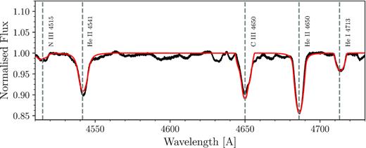
Observed co-added spectrum in black and the best-fitting model according to Table 6 in red. Location and identification for a subset of spectral lines indicated by vertical dashed lines.
The parameters for each generation of models are determined by combining parameters from the previous generation, where models with a lower chi-square have a higher chance of passing their parameters to the next generation. At each generation, parameter variations, or mutations, are introduced to effectively sample the parameter space. The GA analysis was carried out iteratively with the binary modelling (discussed in Section 3.2), where the effective temperature was fixed in the binary modelling first, and then the surface gravity and light-dilution from the binary model was fixed in the next iteration of spectral fitting, until convergence was reached.
We perform an 11 parameter optimization including several stellar parameters: effective temperature (Teff), surface gravity (log g), microturbulent velocity (ξmicro), and macroturbulent velocity (ξmacro); three wind parameters: the mass-loss rate (|$\log \dot {M}$|), the exponent of the wind velocity profile (β), and the terminal wind speed (vinf); and four surface abundance parameters: the helium abundance (YHe), the carbon abundance (ηC), the nitrogen abundance (ηN), and the oxygen abundance (ηO). The helium abundance is given as the ratio of the helium number density to the hydrogen number density while the abundances of carbon, nitrogen, and oxygen are given as the log of the ratio of the elemental number density to the hydrogen number density plus 12. The final optimized values for the fastwind model are listed in Table 6, and the best-fitting model is shown in red in Fig. 8. Our solution results in a primary effective temperature that is nearly 3000 K hotter than determined by Mayer et al. (2013). Furthermore, we note that we find a high microturbulent velocity in HD 165246, whereas previous studies typically fix this quantity. Finally, the macroturbulent velocity reported by the GA optimization is significantly lower than that obtained via the GOF and FT methods previously. This is due to differences in the way that macroturbulence is described, i.e. isotropic in the GOF and FT methods versus anisotropic in fastwind.
Estimated parameters returned from optimized fastwind models.
| Parameter | Unit | Estimate |
|---|---|---|
| Teff | K | |$36\,200^{+900}_{-600}$| |
| log g | dex | |$4.05^{+0.07}_{-0.15}$| |
| |$\log \dot {M}$| | log (M⊙ yr−1) | |$-8.0^{+0.2}_{-0.2}$| |
| β | – | |$0.6787^{+0.15}_{-0.65}$| |
| v∞ | |${\rm km\, s^{-1}}$| | |$2530^{+60}_{-260}$| |
| ξmicro | |${\rm km\, s^{-1}}$| | |$13^{+1.0}_{-1.3}$| |
| ξmacro | |${\rm km\, s^{-1}}$| | |$20^{+5}_{-6}$| |
| vsin i | |${\rm km\, s^{-1}}$| | 268 (fixed) |
| YHe | – | |$0.092^{+0.004}_{-0.004}$| |
| ηC | – | |$8.40^{+0.07}_{-0.04}$| |
| ηN | – | |$7.62^{+0.1}_{-0.09}$| |
| ηO | – | |$8.67^{+0.2}_{-0.01}$| |
5 DISCUSSION
We detect multiple sources of variability in both the spectroscopic and photometric observations of HD 165246. We identify a series of harmonics in the K2 photometry whose base frequency, fp, 2, is also present in the HERMES spectroscopy (fp, 15). The presence of such harmonics in the photometry indicates the presence of non-sinusoidal signal in the data, which in this context has two potential explanations: (i) rotational modulation, or (ii) background binary signal. Given the corroboration of the binary modelling, atmospheric modelling, as well as the identification of this signal in both the photometric and spectroscopic time-series, we argue that this is the result of rotational modulation on the primary O8 V star.
Assigning a single underlying mechanism to the remaining variance in the low-frequency regime is challenging since it contains both coherent p and g modes self-excited via the κ-mechanism as well as stochastically excited IGWs, which may also drive modes at resonant eigenfrequencies (Edelmann et al. 2019; Bowman et al. 2019b; Horst et al. 2020). Given the poor frequency resolution of both the spectroscopic and photometric data sets, we are currently unable to identify the modes/waves. Since we do, however, identify signal in both the photometry and spectroscopy independently, we are able to conclusively state that there is significant pulsational variability present at low frequencies, which originates from the O-type primary. Moreover, the dominant frequencies detected in the moment variations listed in Table 4 all lead to a ratio of the tangential to RV amplitude above unity. This ratio, otherwise known as a K value, can be computed from the mass, radius and frequency of the mode following equation (3.162) in Aerts et al. (2010). This leads to ratios with a range covering roughly [3.3,62.2], meaning that the pulsational variability is dominated by g modes or IGWs as these have dominant tangential motions, while p modes are dominated by radial motions. The signal corresponding to fs, 4 and fs, 10 leads to low K values and may correspond to either low-order p modes (Briquet et al. 2011) or high-order g modes shifted to high frequencies due to the Coriolis force (Buysschaert et al. 2018).
The observed ξmacro variability may have various candidate sources: (i) coherent pulsations, (ii) IGWs, (iii) sub-surface convection, or (iv) stochastic wind variability. As we have identified the presence of pulsations and/or IGWs, these invariably have at least some contribution to the variability in ξmacro on the basis of their contribution to the line profiles from which ξmacro is estimated. The parameters of the O8 V primary place it in a region on the HR diagram where the subsurface convective velocity is theoretically estimated to be below 2.5 km s−1 (Cantiello et al. 2009, see their fig. 9, top panel). Therefore, sub-surface convection cannot fully explain the large and variable tangential velocities that we observe. Furthermore, our estimates of ξmicro, log g, and vsin i place the O-star primary in an underpopulated region of the parameter space to compare with the predictions of Cantiello et al. (2009). This comparison, however, is complicated by the fact that HD 165246 is within the galaxy, whereas the majority of the sample analysed by Cantiello et al. (2009) consists of stars from the Large and Small Magellanic Clouds. In addition, stochastically variable wind signatures as computed by Krtička & Feldmeier (2018) stem from outflow and hence correspond dominantly to radial motions, while the observations point to dominant tangential velocity variations. Our observations of high vsin i, high ξmacro, and the presence of IGWs in the young O-star primary of HD 165246 are consistent with the results of both Simón-Díaz et al. (2017) and Bowman et al. (2019a, 2020). Simón-Díaz et al. (2017) observe a wide range of ξmacro from spectroscopy, and Bowman et al. (2019a) observe a low-frequency excess in photometry (identified as IGWs) in both galactic and LMC O and B stars across the upper HRD. This suggests a common intrinsic mechanism and a relationship between macroturbulence as found in spectroscopy and stochastic low-frequency variability detected in space photometry (Bowman et al. 2020; Burssens et al. 2020)
As demonstrated in Fig. 9, the O8 V primary is located close to the ZAMS in reference to both the non-rotating tracks with different amounts on internal chemical mixing (black tracks), calculated according to Johnston et al. (2019a) using mesa (r-10398; Paxton et al. 2018) as well as tracks with an initial rotational velocity of 40 per cent critical (grey tracks), calculated by Choi et al. (2016) using mesa (r-7503; Paxton et al. 2015). The non-rotating models are calculated such that the internal chemical element mixing is represented in two distinct regimes. The first regime corresponds to the convective boundary mixing (CBM) region, where we represent CBM with diffusive convective overshooting. For overshooting, the free parameter fov scales the slope with which the mixing profile decays beyond the core, as defined by the Schwarzschild criterion in terms of the local pressure scale height, Hp. These models only account for overshooting extending beyond the convective core, and not around any intermediate convective regions in the envelope. The second regime corresponds to radiative envelope mixing (REM), according to the chemical mixing induced by internal gravity waves as derived by Rogers & McElwaine (2017) and implemented in mesa models by Pedersen et al. (2018). In this profile, the free parameter DREM sets the base efficiency of chemical mixing induced by this mechanism, and has units of cm2 s−1. The dashed black (non-rotating) models plotted in Fig. 9 represent the case of minimal internal chemical mixing, with fov = 0.005 and DREM = 10 cm2 s−1. The dash–dotted black (non-rotating) models represent the case of maximum internal mixing with fov = 0.04 and |$D_{\rm REM}=10\, 000$| cm2 s−1. These limiting values are those deduced by asteroseismology of intermediate-mass g-mode pulsating field stars (Briquet et al. 2007; Daszyńska-Daszkiewicz & Walczak 2010; Daszyńska-Daszkiewicz, Szewczuk & Walczak 2013; Moravveji et al. 2016; Schmid & Aerts 2016; Buysschaert et al. 2018; Walczak et al. 2019; Wu & Li 2019). Despite the differences in the form of internal mixing between the two sets of evolutionary tracks, comparison of the observations with both tracks reveals a massive primary that has consumed less than 30 per cent of its initial core hydrogen content, as seen in Fig. 9.
Evolutionary tracks for 25-, 20-, 15-, and 10-M⊙ models. Solid black line denotes the zero-age main sequence (ZAMS) line. Black tracks taken from Johnston et al. (2019a) with fov = 0.005, DREM = 10 cm2 s−1 (dashed lines) and fov = 0.040, |$D_{\rm REM}=10\, 000$| cm2 s−1 (dash–dotted lines). Black tracks have Y = 0.276, Z = 0.0140, and use OP opacities. Solid grey tracks are MIST Stellar evolution tracks taken from Choi et al. (2016) with vZAMS/vcrit = 0.4, Y = 0.2703, Z = 0.0142, and OPAL opacities, for the same masses.
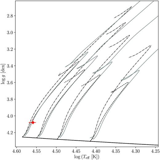
Fig. 10 compares the dynamical mass and surface gravity estimates for the O8V primary of HD 165246 with theoretical isochrones with different amounts of internal mixing using models calculated using mesa (Paxton et al. 2018) by Johnston et al. (2019a). The location of HD 165246A in Fig. 10 indicates that it has an age between 2 and 3 Myr and a core hydrogen content of Xc = 0.54, given the uncertainties on the dynamical surface gravity (black), or an age between 2 and 4.5 Myr, given the uncertainties on the spectroscopic surface gravity (red). Our age estimates agree with those of Mayer et al. (2013), who used evolutionary tracks from Brott et al. (2011). The overlap between the dynamical and spectroscopic surface gravity estimates provides support for the mass estimate derived for the primary component. However, given the inability to detect the secondary star in the spectra, we have no means of independently verifying the solution for the secondary, making us wary of its absolute dimensions. With this in mind, we find that the secondary is not yet on the main sequence when compared to the isochrones in Fig. 10. We note that without smaller uncertainties on the parameters of the primary, we are not able to constrain the impact of internal chemical mixing on the evolution of this star. Additionally, without proper characterization of the secondary via detection of its RV variations, we are not able to perform isochrone-cloud fitting as introduced by Johnston, Pavlovski & Tkachenko (2019b) and applied by Tkachenko et al. (2020).
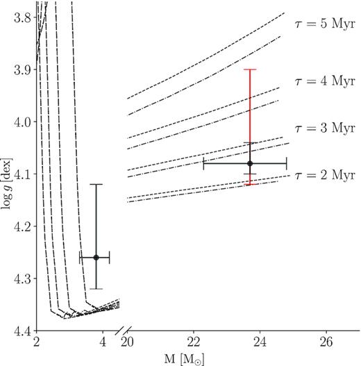
Isochrones for 2, 3, 4, and 5 Myr shown in grey for tracks with fov = 0.005, DREM = 10 cm2 s−1 (dashed lines), and fov = 0.040, |$D_{\rm REM}=10\, 000$| cm2 s−1 (dash–dotted lines). All models have Y = 0.276 and Z = 0.014 and OPAL opacities. Dynamical (spectroscopic) estimates for mass and log g denoted by black (red) error-bars.
6 CONCLUSIONS
This work made use of an extensive set of new time-series spectroscopy to build upon the work by Mayer et al. (2013) and Johnston et al. (2017) for a more in-depth study of the massive eclipsing O+B binary HD 165246. Using this spectroscopy, we obtained updated atmospheric and binary solutions revealing an effective temperature of |$T_{\rm eff} = 36\, 000$| K and a mass of M = 23.7 M⊙ for the O-star primary. Furthermore, we determine a rotation rate of vsin i = 268 km s−1, microturbulence of ξmicro = 13 km s−1, and variable macroturbulence linked to time-dependent pulsational line-broadening. We explored the variability detected in both the K2 photometry and hermes spectroscopy, and find it consistent with rotational modulation, as well as intrinsically excited stellar pulsations.
The presence of pulsational variability in the light curve and hermes spectroscopy provide at least a partial explanation for the high macroturbulence derived from the atmospheric modelling. This is consistent with the predictions of Aerts et al. (2009), 2014) and the observations of Simón-Díaz et al. (2017). The evolutionary status of the O8V primary is consistent with expectations from models. Higher precision on the fundamental stellar parameters is required for scrutinizing evolutionary models at masses and ages typical of O-stars. However, the observed atmospheric properties of the primary component situate this star in an underpopulated region of the parameter space of massive star variability studies.
High-mass eclipsing binaries such as HD 165246 are integral to the study of variability in the upper regions of the HRD. The characterization of such systems is required to provide benchmarks for hydrodynamical simulations and evolutionary codes. Currently, the community lacks the sample size of well-characterized high-mass stars (including fundamental parameters) required to discriminate between the physical mechanisms proposed as the causes of observed variability. The TESS (Ricker et al. 2015) is currently assembling sub-mmag precision space-based photometry of high-mass stars across the entire sky. This sample is yielding high-quality observations of more massive stars than any homogeneous data base to date (see e.g. Burssens et al. 2020; Labadie-Bartz et al. 2020). Characterization of the variability (or lack thereof) in these stars is providing the basis upon which predictions of physical mechanisms can be tested. In particular, stars that reveal coherent oscillation modes whose degree and azimuthal order can be identified, are suitable to be probeb via asteroseismology (Bowman 2020; Aerts 2021). So far, such detections and identifications are typically achieved in only about 10 per cent of the observed OB-type stars, but this fraction is expected to increase, thanks to TESS.
ACKNOWLEDGEMENTS
We thank the referee for their comments that improved this paper. The research leading to these results has received funding from the European Research Council (ERC) under the European Union’s Horizon 2020 research and innovation programme (grant agreement N○670519: MAMSIE and grant agreement N○772225: Multiples), from the KU Leuven Research Council (grant C16/18/005: PARADISE and C16/17/007: MAESTRO), from the Research Foundation Flanders (FWO) under grant agreements G0H5416N (ERC Runner Up Project) and G0A2917N (BlackGEM), from the FWO-Odysseus program under G0F8H6N, as well as from the BELgian federal Science Policy Office (BELSPO) through PRODEX grant PLATO. DMB gratefully acknowledges a senior postdoctoral fellowship from the Research Foundation Flanders (FWO) with grant agreement No. 1286521N. The computational resources and services used in this work were provided by the VSC (Flemish Supercomputer Center), funded by the Research Foundation Flanders (FWO) and the Flemish Government – department EWI to PI Johnston.
This paper is based on observations obtained with the HERMES spectrograph on the Mercator telescope, which is supported by the Research Foundation Flanders (FWO), Belgium, the Research Council of KU Leuven, Belgium, the Fonds National de la Recherche Scientifique (FRS-FNRS), Belgium, the Royal Observatory of Belgium, the Observatoire de Genéve, Switzerland, and the Thüringer Landessternwarte Tautenburg, Germany
DATA AVAILABILITY
The K2 data presented in this paper were obtained from the Mikulski Archive for Space Telescopes (MAST) at the Space Telescope Science Institute (STScI), which is operated by the Association of Universities for Research in Astronomy, Inc., under NASA contract NAS5-26555. Support to MAST for these data is provided by the NASA Office of Space Science via grant NAG5-7584 and by other grants and contracts. Funding for the Kepler/K2 mission was provided by NASA’s Science Mission Directorate. The hermes data used within this paper are available upon request. The binary modelling was carried out using ellc (Maxted 2016) and the atmospheric modelling was carried out using fastwind (Puls et al. 2005). The propagation of asymmetric uncertainties was performed using the soad code (Erdim & Hüdaverdi 2019). The optimization routines in this work made use of the numpy (Harris et al. 2020) and emcee (Foreman-Mackey et al. 2013), and the plotting was carried out using matplotlib (Hunter 2007). Mode identification results obtained with the software package famias developed in the framework of the FP6 European Coordination Action HELAS (http://www.helas-eu.org/).
REFERENCES
APPENDIX A: MOMENT METHOD PERIODOGRAMS
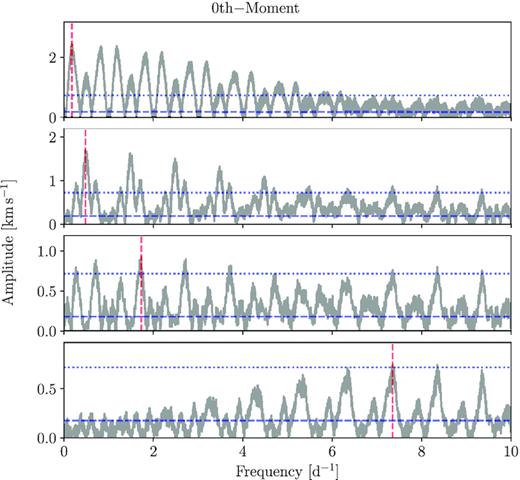
Periodograms of the zeroth-moment of the LSD profiles. Extracted frequencies denoted by red vertical line. Dashed blue lines show noise level of pre-whitened data set, and dotted blue lines denote four times the noise level.
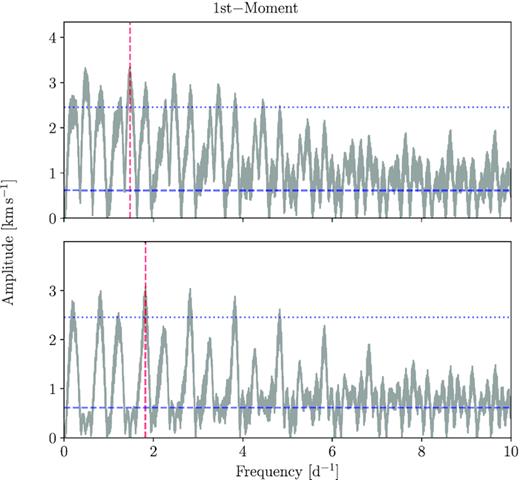
Same as Fig. A1 but for the first moment.
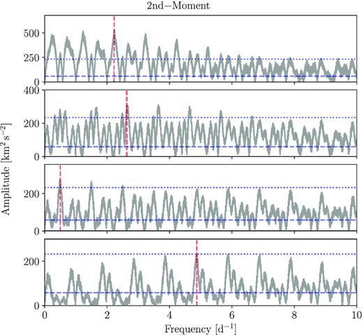
Same as Fig. A1 but for the second moment.
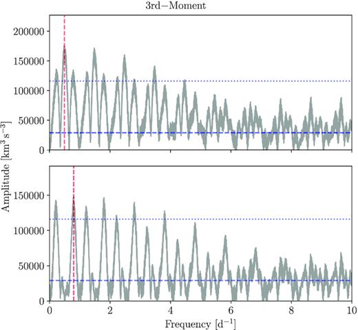
Same as Fig. A1 but for the third moment.
