


ABSTRACT
A promising route for revealing the existence of dark matter structures on mass scales smaller than the faintest galaxies is through their effect on strong gravitational lenses. We examine the role of local, lens-proximate clustering in boosting the lensing probability relative to contributions from substructure and unclustered line-of-sight (LOS) haloes. Using two cosmological simulations that can resolve halo masses of Mhalo ≃ 109 M⊙ (in a simulation box of length |$L_{\rm box}{\sim }100\, {\rm Mpc}$|) and 107 M⊙ (|$L_{\rm box}\sim 20\, {\rm Mpc}$|), we demonstrate that clustering in the vicinity of the lens host produces a clear enhancement relative to an assumption of unclustered haloes that persists to |$\gt 20\, R_{\rm vir}$|. This enhancement exceeds estimates that use a two-halo term to account for clustering, particularly within |$2-5\, R_{\rm vir}$|. We provide an analytic expression for this excess, clustered contribution. We find that local clustering boosts the expected count of 109 M⊙ perturbing haloes by |$\sim \! 35{{\ \rm per\ cent}}$| compared to substructure alone, a result that will significantly enhance expected signals for low-redshift (zl ≃ 0.2) lenses, where substructure contributes substantially compared to LOS haloes. We also find that the orientation of the lens with respect to the line of sight (e.g. whether the line of sight passes through the major axis of the lens) can also have a significant effect on the lensing signal, boosting counts by an additional |$\sim 50{{\ \rm per\ cent}}$| compared to a random orientations. This could be important if discovered lenses are biased to be oriented along their principal axis.
1 INTRODUCTION
The large-scale clustering of galaxies provides important constraints on the makeup and evolution of the Universe (e.g. Geller & Huchra 1989; Bond, Kofman & Pogosyan 1996; Tegmark et al. 2004; Sánchez et al. 2006). The dark energy plus cold dark matter (CDM) paradigm, ΛCDM, is entrenched as the benchmark model for the theory of galaxy formation based largely on its success in matching observed large-scale structure. For years, cosmological N-body simulations that incorporate only gravitational dynamics (dark matter only, DMO, simulations) have served as crucial tools for understanding the ΛCDM model, and have been used to understand the detailed clustering of galaxies. When introducing full galaxy formation physics, cosmological simulations are able to match observed clustering statistics as a function of galaxy type as well (e.g. Genel et al. 2014; Vogelsberger et al. 2014; Khandai et al. 2015; Schaye et al. 2015; Dubois et al. 2016; Dolag, Komatsu & Sunyaev 2016; Springel et al. 2018; Vogelsberger et al. 2020) however some discrepancies on smaller scales exist and motivate the exploration of alternative models (Bullock & Boylan-Kolchin 2017; Meneghetti et al. 2020).
A feature of CDM that profoundly separates it from many other dark matter models is that CDM predicts a rich abundance of low-mass dark matter haloes Mhalo < 106 M⊙ (Press & Schechter 1974; Bullock & Boylan-Kolchin 2017). In cosmologies that include warm dark matter (WDM), for example, the power spectrum is suppressed on scales smaller than a value set by the WDM particle mass (Bode, Ostriker & Turok 2001; Bozek et al. 2016). For a thermal WDM particle of mass |$m_{\rm thm} \lesssim 5\ \rm kev$|, the formation of haloes <107 M⊙ (e.g. Schneider, Smith & Reed 2013; Horiuchi et al. 2016) is suppressed. Therefore, if haloes below ≃107 M⊙ are detected, this would impose significant constraints on both the dark matter power spectrum and the particle nature of dark matter (see Bertone & Tait 2018).
Dark matter haloes of sufficiently low mass are expected to be unable to form stars or retain baryons in the presence of a cosmological photoionizing background (e.g. Efstathiou 1992; Bullock, Kravtsov & Weinberg 2000). The detection of these starless haloes, with the abundance and density structure predicted by simulations, would be triumphant for the CDM model. One way of inferring the presence of these low-mass objects is by their influence on cold, low-velocity stellar streams in the Milky Way (Ibata et al. 2002; Carlberg 2009; Yoon, Johnston & Hogg 2011). Recently Banik et al. (2019) argued that the observed perturbations of the MW’s stellar streams can only be explained by a population of subhaloes in CDM. They set constraints to alternative dark matter models for haloes down the mass function, notably setting a lower limit on the mass of warm dark matter thermal relics |$m_{\rm thm} \gtrsim [4.6-6.3]\ \rm keV$|. In order to provide tighter constraints for substructure down to Mhalo ≃ 105–6M⊙ populating the MW, a larger sample cold streams would be needed. Another proposed approach to detecting these low-mass haloes could be through the kinematics of stars in the Milky Way’s disc (Feldmann & Spolyar 2015).
Currently, the field of strong gravitational lensing offers to be another tool for the indirect detection of low-mass, starless haloes of masses ≃106–8 M⊙ (Dalal & Kochanek 2002; Koopmans 2005; Vegetti et al. 2010, 2014; Li et al. 2016; Nierenberg et al. 2017). Lensing perturbations can arise from both subhaloes within the lens host and from small haloes found outside of the virial radius that perturb the light from source to the observer (dubbed ‘line-of-sight’ (LOS) haloes; Li et al. 2017; Despali et al. 2018). Notably, the field of substructure lensing offers tantalizing prospects, as in the near future, we expect both a gross increase in the number of lenses as well as a boost in resolution for instrument sensitivity. Forecasts suggest that the Dark Energy Survey (DES), LSST, and EUCLID should discover hundreds of thousands of galaxy–galaxy lensing systems (Collett 2015). The Nancy Grace Roman Space Telescope (RST) also has the potential of providing complementary catalogues of lens images (Weiner, Serjeant & Sedgwick 2020). Additionally, the detection of haloes with Mhalo ∼ 107–8 M⊙ might be possible with JWST via quasar flux ratio anomalies (MacLeod et al. 2013). As of now, reported detections using ALMA reach the mass scale of classical Milky Way satellites (Mhalo ∼ 1010M⊙), with constraints on subhaloes an order of magnitude smaller. In the future, further observations and improved constraints may significantly improve these limits (Hezaveh et al. 2016) and offer tighter constraints on the warm dark matter mass (He et al. 2020), especially when combined with Milky Way satellite constraints (Nadler et al. 2021).
The expected count of subhaloes that exist within the virial radius of the lens system has been studied rigorously. Studies of subhalo populations and their effect on lensing have previously relied on DMO simulations (e.g. Bradač et al. 2002; Xu et al. 2009, 2012; Metcalf & Amara 2012; Vegetti et al. 2014). More recently, however, simulations that implement full galaxy formation physics show that small subhaloes are actually depleted with respect to DMO simulations, owing to interactions with the central galaxy (Brooks & Zolotov 2014; Wetzel et al. 2016; Zhu et al. 2016; Graus et al. 2018; Kelley et al. 2019; Richings et al. 2021). Notably, Garrison-Kimmel et al. (2017) showed that it is the central galaxy potential itself, not feedback, that drives most of the factor of ∼2 difference in subhalo counts between DMO and full physics simulations for Milky Way-mass haloes (Mvir ≃ 1012 M⊙). For lens-mass haloes of interest (Mvir ≃ 1013 M⊙), Despali & Vegetti (2017) used both DMO and full physics from the EAGLE (Schaye et al. 2015) and Illustris (Vogelsberger et al. 2014) simulations to investigate predictions for subhalo lensing and found that simulations with full galaxy formation physics reduces the average expected substructure counts. The substructure analysis done in Graus et al. (2018) using Illustris found similar results.
Given the expected depletion in subhalo counts seen in full-physics simulations, the contribution of lensing signals from LOS haloes has been recognized as ever more important. If LOS haloes dominate the signal from a given lens, then uncertainties are reduced substantially because the contribution of the LOS haloes can be accurately calculated, independent of the effect of baryonic physics, for a variety of cosmologies. Efforts have been made to understand the contribution of the LOS structure on the flux ratio anomalies in lensed quasars (e.g. Metcalf 2005; Inoue & Takahashi 2012; Metcalf & Amara 2012; Xu et al. 2012; Inoue et al. 2015; Xu et al. 2015; Inoue 2016; Gilman et al. 2018, 2019). It has become increasingly apparent that LOS haloes should dominate the signal for more distant lenses (zl ∼ 0.5) while the contribution from subhaloes should be non-negligible for more local lenses (zl ∼ 0.2; Despali & Vegetti 2017).
Our objective in this article is to understand and quantify an effect not discussed in most previous work: how does local, correlated structure, in the vicinity of the lens host halo, impact the expected lensing signal? While such an effect has been discussed before in the context of weak lensing (D’Aloisio, Natarajan & Shapiro 2014), its impact in strong lensing remains elusive. This effect will be most important for low-redshift lenses, where subhaloes are known to contribute non-trivially compared to the LOS count. We use a suite cosmological simulations, including those that include both DMO and full galaxy formation physics, to explore this question. Specifically, we quantify correlated structure in lens-centred projections of targets lens haloes of |$M_{\rm vir}\simeq 10^{13}\, M_{\odot }$| at redshift z = 0.2, corresponding with the benchmark sample discussed in Vegetti et al. (2014). This is done using two simulation projects: The first, from the public IllustrisTNG project (Nelson et al. 2018), includes both DMO and full-physics versions and resolves haloes down to |$M_{\rm halo} = 10^{9}\, M_{\odot }$| in a fairly large cosmological volume. The second is a DMO simulation evolved in much smaller cosmological volume that is able resolve dark matter haloes down to |$M_{\rm halo} = 10^{7}\, M_{\odot }$|.
This paper is structured as follows. Section 2 introduces our set of simulations, provides a description of the selected sample of haloes, and outlines our methodology for counting structures along projected line of sights in the simulations. Section 3 provides results on structure and explores how the lens-host orientation can boost the amount of structure expected along lens-centred projections. Finally, we summarize our results in Section 4. Note that in strong lensing literature, terms such as ‘field halo’ and ‘line-of-sight (LOS) halo’ typically refer to the same things. We will use these terms interchangeably throughout this work to refer to haloes having a volume density equal to the cosmological mean density of haloes at that mass.
2 NUMERICAL METHODOLOGY
Our ΛCDM predictions rely on two sets of simulations. The primary set comes from the public catalogues of the IllustrisTNG project1 (Marinacci et al. 2018; Naiman et al. 2018; Nelson et al. 2018; Pillepich et al. 2018; Springel et al. 2018). As described in Section 2.1, these simulations allow us to identify halo populations robustly to masses greater than 109 M⊙ for a large-scale environment both with gravitational physics alone and with full galaxy formation physics. The second simulation, introduced in Section 2.2, is a DMO version of a new simulation suite called FIREbox, which is part of the Feedback in Realistic Environments (FIRE) project.2 The mass functions of these simulations are presented in Fig. 1. Both simulations assume a Planck 2015 cosmology (Planck Collaboration XIII 2016): Ωm = 0.3089, ΩΛ = 0.6911, Ωb = 0.0486, σ8 = 0.8159, and h = 0.6774.
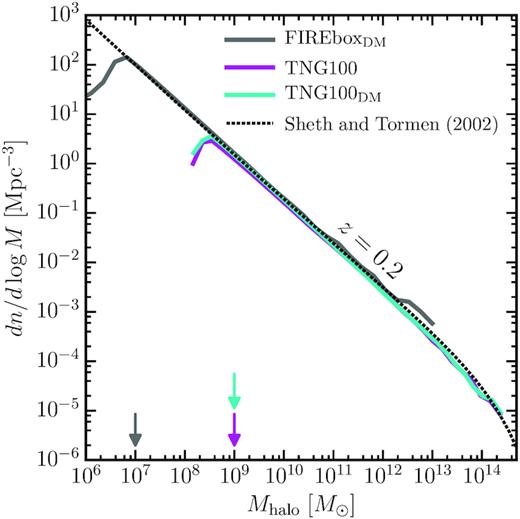
The abundance of resolved dark matter haloes. Shown are the halo mass functions of the simulations at z = 0.2. Results from all three simulation are in agreement with the analytical prediction of Sheth & Tormen (2002). The arrows pointing to the x-axis designate the minimally resolved mass considered in each simulation, indicated by the colour coding.
Our analysis relies on halo catalogues at redshift z = 0.2, which coincides with a typical redshift of the lens–host sample explored in Vegetti et al. (2014). Dark matter haloes are defined to be spherical systems with a virial radius, Rvir, inside which the density is equal to the average density of Δvir(z)ρcrit(z), where Δvir(z) is the virial overdensity defined by Bryan & Norman (1998) and ρcrit(z) is the critical density of the Universe. The virial mass, Mvir, is then the total mass enclosed in a sphere of radius Rvir.
In what follows, we discuss two types of haloes: First, we have massive target haloes, chosen to mimic lens–galaxy hosts: Mvir ∈ [0.8 − 2] × 1013 M⊙. Secondly, we have low-mass perturber haloes, which can either be subhaloes or small haloes that exist somewhere outside of the host’s virial radius and along the LOS from the observer. We quote their masses (taken from the halo catalogues) using the symbol Mhalo, since for subhaloes Mvir is not physically relevant.
2.1 The IllustrisTNG simulations
The IllustrisTNG (TNG) suite of cosmological simulations was run using the moving-mesh code arepo (Springel 2010). The runs with full galaxy formation physics use an updated version of the Illustris model (Weinberger et al. 2017; Pillepich et al. 2018). We use the high resolution set of publicly available simulations,3 TNG100-1, which has a comoving box of side length |$L_{\rm box}^{\rm TNG}=75\, h^{-1} \mathrm{cMpc}=110.7\, {\rm cMpc}$|. The full physics run, TNG100, has a dark matter particle mass of mdm = 7.5 × 10⁶ M⊙ and a gas particle mass of mgas = 1.4 × 10⁶ M⊙. The high-resolution simulation that uses dark matter only (DMO) physics, TNG100DM, has the same box size, but treats baryonic matter as collisionless particles, which gives the simulation a particles mass is mdm = 8.9 × 10⁶ M⊙. When comparing between TNG100 and TNG100DM, we account for the excess baryonic mass in the DMO simulation by introducing a factor mdm → (1 − fb)mdm, where fb ≔ Ωb/Ωm is the cosmic baryon fraction.
For both TNG100 and TNG100DM, the dark matter halo catalogues were constructed using a friends-of-friends (fof) algorithm (Davis et al. 1985) with a linking length 0.2 times the mean interparticle spacing. Gravitationally bound substructures are identified through the subfind halo finder (Springel et al. 2001). These subhaloes have a dark matter mass that is gravitationally bound to itself but not to any other subhaloes found in the same fof host or the host itself. As shown in Fig. 1, the z = 0.2 mass functions of the TNG100 (magenta) and TNG100DM (cyan) subfind subhaloes match well with the analytical (Sheth & Tormen 2002) mass function (dotted dashed) at that redshift. Both simulations become incomplete just below Mhalo ≃ 108.6 M⊙. In order to be conservative, we restrict our analysis to subhaloes and field haloes with resolved masses Mhalo > 109 M⊙. These haloes contain at least 134 dark matter particles. TNG100 and TNG100DM have 166 and 168 lens–target haloes, respectively, where in TNG100, these haloes typically host galaxies with M⋆ ≃ 1011 M⊙, which is consistent with the benchmark sample in Vegetti et al. (2014).
The public subfind catalogues in TNG100 include several baryon-dominated ‘subhaloes,’ many of which contain no dark matter. Most of these baryon-dominated objects exist within ∼20 kpc of host galaxies and appear to be baryonic fragments numerically identified by subfind rather than galaxies associated with dark matter subhaloes. While baryonic clumps could induce perturbations detectable in lens images (Gilman et al. 2017; Hsueh et al. 2017, 2018; He et al. 2018), this type of object is not the focus of our analysis; we are interested in the search for low-mass dark matter structures. For this reason, we exclude systems with a ratio of total baryonic mass to dark matter mass that is more that twice the cosmic baryon fraction, (Mbar/Mhalo > 2 × fb) in the substructure analysis that follows.
2.2 The FIREbox DMO simulation
FIREbox is a new effort within the FIRE collaboration to simulate cosmological volumes of |$L_{\rm box}^{\rm FIRE} = 15\ h^{-1}\rm cMpc = 22.14\ cMpc$| at the resolution of FIRE zoom-in simulations (Feldmann et al., in preparation). Our analysis uses the results from a DMO version of the FIREbox initial conditions, ran with 20483 particles, which we dub FIREboxDM in this article. FIREboxDM has a dark matter particle mass of mDM = 5.0 × 10⁴ M⊙ and was run with a Plummer softening length of |$\epsilon _{\rm DM} = 40\ \rm pc$|. Since we will work with a DMO simulation to complement the analysis done in the two TNG simulations, we again account for baryonic mass by multiplying a by conversion factor of (1 − fb), as we do for TNG100DM.These simulations are complete, conservatively, to halo masses down to 107 M⊙ (see Fig. 1).
The halo catalogue for FIREboxDM was generated using rockstar (Behroozi, Wechsler & Wu 2013). This method finds dark matter haloes using a hierarchically adaptive refinement of fof in a 6D phase-space and one time dimension. We set our rockstar halo finding parameters to be comparable to those use in the TNG catalogues generated by subfind. Specifically, we use an fof linking length of b = 0.20 and include only haloes that have at least 100 dark matter particles. We also set the criteria for unbound particle fraction rejection to |$70{{\ \rm per\ cent}}$| instead of the default |$50{{\ \rm per\ cent}}$|, as explored in the Appendix of Graus et al. (2018). Doing so minimizes ambiguities associated with using different halo finders for computing halo masses.4 With these choices, FIREbox contains three target haloes with mass Mvir ∈ [0.8 − 2] × 1013 M⊙.
Returning to Fig. 1, the mass function of FIREboxDM at z = 0.2 is shown as the solid grey curve and agrees well with the analytical mass function down to halo masses with 107–8 M⊙. With this in mind, the use of FIREboxDM in our analysis will be restricted to two sets of subhalo masses: a sample of halo masses down to 107 M⊙ (∼102 particles) and a sample of down to 108 M⊙ (∼103 particles). For a more stringent check, Appendix C compares the subhalo mass function and the subhalo Vmax function of the three target-lens haloes of FIREboxDM to the same mass target-lens haloes in TNG100DM. We find excellent agreement between substructure statistics between our halo samples.
2.3 Counting within lens-centred cylinders
We quantify perturber counts by enumerating small haloes that sit within randomly oriented lens-centred cylinders of length ℓ and radius |$\mathcal {R}$|, where ℓ can extend over the length of the simulation box and |$\mathcal {R}$| will be set to a value close to an expected Einstein radius (∼10 kpc). As illustrated in Fig. 2, each cylinder is centred on a target halo in the simulation box. The volume of the cylinder is increased by lengthening ℓ → ℓ + Δℓ with the radius |$\mathcal {R}$| fixed. For a discrete increment variation of Δℓ, both ends of the cylinder are increased by (Δℓ)/2, which captures both structures whose positions are found in the foreground and background of the target halo. Doing so allows us to qualitatively compare counts as function of radius r from the halo centre, i.e. r ≃ ℓ/2. For example, a lens-centred cylinder length of ℓ = 2Rvir spans the full diameter of the dark matter halo.
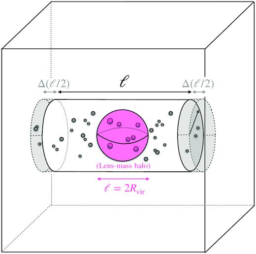
A cartoon depiction of the analysis we perform for each lens-centred cylinder in a simulation box. The lens–mass halo, centred at the origin of the box, is illustrated as the large pink sphere, while subhaloes are illustrated as smaller haloes. With the cylinder held at a fixed |$\mathcal {R}$|, the cylinder is varied by increments of Δℓ (Δℓ/2 at each end of the cylinder) until reaching the edge of the box. Note that the radius of the cylinder has been exaggerated for clarity. In practice, |$\mathcal {R} \ll R_{\rm vir}$|.
In what follows we compare counts from lens-centred cylinders to those of average cylinders, which are configured like a lens-centred cylinder, but now with their centres randomly placed within the simulation box. Note for a large sample of average cylinders, the mean count per unit volume at any ℓ will be equal to the average halo density (e.g. Sheth & Tormen 2002). For both cylinder types, we take into account the periodicity of the cosmological box but never allow the full cylinder length to exceed the box length.
Fig. 3 provides a simple illustration of our counting prescription applied to TNG100 for a single lens–mass halo of Mvir ≃ 1013M⊙ (labelled as ‘lens-centred cylinder’) and for a randomly placed cylinder of the same size inside the box (labelled as ‘average cylinder’). For illustrative purposes, we have set the radius of the cylinder to a very large value |$\mathcal {R} = R_{\rm vir} \simeq 500\ \rm kpc$|, much larger than what we will use in our main analysis. The cylinder length is set to |$\mathcal {\ell }=10$| Mpc. The filled circles show all subhaloes with Mhalo > 109 M⊙. Points and circles are coloured based on their relative distance from the host: within ℓ = 2Rvir (r = Rvir) as cyan, ℓ = [2 − 4]Rvir (r = [1 − 2]Rvir) as magenta, and black for everything else out to a length ℓ = 10 Mpc. The two top plots show the edge-on projections while the bottom plots are the face-on projections. For the face-on projections, the sizes of the circles are scaled proportionally to the mass of the haloes in the cylinder (with the host halo removed for clarity). In the bottom left-hand panel, we show only haloes that are outside of Rvir of the lens host. Even excluding substructure, the overall count is much higher than the random cylinder.
![The importance of correlated structure in sub-galactic lensing. The upper and middle panels depict the side-view of a cylinder length of $\ell = 10\ \rm Mpc$ and radius $\mathcal {R} = 500\ \rm kpc$ centred on a lens–mass host halo with radius $R_{\rm vir} \simeq 500\ \rm kpc$ at z = 0.2 in the TNG100 simulation. The points show locations of Mhalo > 109 M⊙ haloes within the cylinder, colour coded by relative distance from the host out to the size of the halo ℓ = 2Rvir (or equivalently to r = Rvir; cyan points), within ℓ = [2 − 4]Rvir (r = [1 − 2]Rvir; magenta points), and everything else outside ℓ = 4Rvir out to ℓ = 10 Mpc (black points). The figure beneath it shows an identical cylinder that samples a representative region of the simulation box using the same colour scheme; the area of each point is proportional to that halo’s mass. The square plots are the same cylinders shown face on, centred on the lens (left-hand panel) and centred randomly (right-hand panel). The cylinder radius $\mathcal {R}=500\, {\rm kpc}$ used for this figure is, for illustrative purposes, much larger than the typical Einstein radius of the host ($\mathcal {R} \approx 10\, {\rm kpc}$; we use the latter value for our actual analysis. Local, correlated perturbers around the lens are highly significant (compare the magenta points in the left-hand verses right-hand panels on the bottom).](https://oup.silverchair-cdn.com/oup/backfile/Content_public/Journal/mnras/502/4/10.1093_mnras_stab448/1/m_stab448fig3.jpeg?Expires=1750054832&Signature=DQ5z29ul66H6QyIqO1~cAHXlU8qJscDFYviZYyBUSnxxbkZZyFVzefwnDmWZC9FIJmrBbnuhL4rhB2pr1wnDFCeYzPcMZug5N~S4et~OvgNtFj0Jve7rR~1JOVWCOskG971tRhV~3wDaRFC5hTJhDE~5bqrul~Dxcw~1BxqB5tATEMdeXfF4dEdlWl5z-gwmK3JKvEYWsRMwRAQzQhPOhzBxURxBWzGMlP1i1gOSs4TUG3oqvr-iT2XA8wIYK7Z-kSNoDqy3QcvZlPDl9nnGhoqCSaqIv45io17UFQL4O1Ue4CRL~DLay0njcS~3vCSqtWRUvNyEXMd8FrpIgduapQ__&Key-Pair-Id=APKAIE5G5CRDK6RD3PGA)
The importance of correlated structure in sub-galactic lensing. The upper and middle panels depict the side-view of a cylinder length of |$\ell = 10\ \rm Mpc$| and radius |$\mathcal {R} = 500\ \rm kpc$| centred on a lens–mass host halo with radius |$R_{\rm vir} \simeq 500\ \rm kpc$| at z = 0.2 in the TNG100 simulation. The points show locations of Mhalo > 109 M⊙ haloes within the cylinder, colour coded by relative distance from the host out to the size of the halo ℓ = 2Rvir (or equivalently to r = Rvir; cyan points), within ℓ = [2 − 4]Rvir (r = [1 − 2]Rvir; magenta points), and everything else outside ℓ = 4Rvir out to ℓ = 10 Mpc (black points). The figure beneath it shows an identical cylinder that samples a representative region of the simulation box using the same colour scheme; the area of each point is proportional to that halo’s mass. The square plots are the same cylinders shown face on, centred on the lens (left-hand panel) and centred randomly (right-hand panel). The cylinder radius |$\mathcal {R}=500\, {\rm kpc}$| used for this figure is, for illustrative purposes, much larger than the typical Einstein radius of the host (|$\mathcal {R} \approx 10\, {\rm kpc}$|; we use the latter value for our actual analysis. Local, correlated perturbers around the lens are highly significant (compare the magenta points in the left-hand verses right-hand panels on the bottom).
For this particular randomly chosen ‘average’ cylinder, we find 14 haloes with Mhalo > 109 M⊙ within the 10 Mpc projection visualized. Note that the cosmological average expected for this volume is ≈14.3 when using the Sheth & Tormen (2002) mass function. Counts are significantly higher for the lens-centred cylinder. For comparison, the lens-centred cylinder contains 108 haloes of the same mass. Interestingly, correlated structure counts around the lens–host that exist outside of r = Rvir but within r = 2Rvir is 28, which exceeds all of the counts within the 10 Mpc long average cylinder. This shows that clustering in the vicinity of the lens will boost signals non-trivially compared to what we would have estimated by ignoring local clustering outside of the halo virial radius.
While Fig. 3 is useful to elucidate the point of a projected cylinder, the radius shown, |$\mathcal {R} = R_{\rm vir}$|, is not relevant for lensing studies. The remainder of the analysis hereafter imposes a fixed projected cylinder radius of |$\mathcal {R} = 10\ \rm kpc$|, which is a value comparable to size of the lens–mass’ Einstein radius (typically ≲10 kpc). Note that in the SLACS sample used by Vegetti et al. (2014) at a redshift 〈zlens〉 ∼ 0.2, the median Einstein radius is ∼4.2 kpc. We adopt a slightly larger 10 kpc radius in what follows in order to improve counting statistics (see Appendix A1 for a discussion of counting variance). Our primary results below are framed as relative counts per unit volume, such that the precise radius of the cylinder factors out. We show in Appendix A2 that our results are insensitive (to within counting noise) to choices of cylinder radii of 5 kpc and even 2 kpc.
3 RESULTS
3.1 Average halo counts in projection
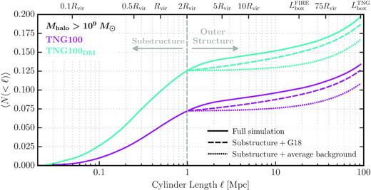
Our main results are presented in Fig. 4, where we plot the mean differential count of haloes per cylinder length, 〈dN/dℓ〉 using 100 cylinders randomly oriented around each lens–mass halo (solid lines). Integrating dN/dℓ over ℓ gives the cumulative count N(< ℓ) within a cylinder of total length ℓ. We plot the differential count as a function of cylinder length, ℓ. Shown is the mean differential count rather than the median because this allows us to compare directly to analytic expectations for the average halo abundance. Each solid curve shows the rate of counts for halo masses greater than a given value (indicated in the legend), normalized by the rate of counts expected from the average background from Sheth & Tormen (2002). Counts equal to the rate of counts from the average background are shown as the horizontal dotted line with an amplitude of 1.5 The vertical grey-dashed line separates between the two regimes of interest: the substructure contribution (ℓ < 2Rvir and the local structure (ℓ > 2Rvir).
![Structure excess along lens-centred projections: The mean differential count 〈dN/dℓ〉 of small haloes within cylinders of increasing length ℓ + Δℓ centred on the lens–mass host haloes (Mvir ≃ 1013M⊙, solid coloured), normalized by the expected average background counts via Sheth & Tormen (2002) halo mass function (dotted black). The cylinders mirror those shown in Fig. 3, but now with a radius comparable to the Einstein radius of the lens–mass haloes, $\mathcal {R} = 10\ \rm kpc$ (and varying length ℓ). The grey vertical dashed line marks the typical outer region of the halo (ℓ = 2Rvir↔r = Rvir). Inside the lens–mass host haloes (ℓ < 2Rvir), the differential counts are self-similar for the DMO simulations. For TNG100 (solid magenta), the counts decrease by almost a factor of 10 because of the destructive effect of the central galaxy. Differences between the curves become apparent outside the halo due to local halo clustering. This effect originates predominantly from ‘backsplash’ haloes that have pericentres with r < Rvir but apocentres of r > Rvir, meaning they lie within the splashback radius of the lens–mass host but spend most of their time at r > Rvir. For comparison, we plot the analytical contribution of the two-halo term given by G18 (equation 1; dashed orange), where we set δlos = 1. While G18 accurately reproduces the contribution at ℓ > 5 × Rvir for most of the curves, it significantly underpredicts the differential halo counts within ℓ ∈ [2 − 5]Rvir. Our proposed modification, equation (3) (dashed black), captures the excess for $\ell \gt 2\, R_{\rm vir}$ to within $10{{\ \rm per\ cent}}$.](https://oup.silverchair-cdn.com/oup/backfile/Content_public/Journal/mnras/502/4/10.1093_mnras_stab448/1/m_stab448fig4.jpeg?Expires=1750054832&Signature=JQRHaLhNkNF2-CsKsgkp06WI2zkhQq3sJynAgosFg-Lkix8SknGxJ-HvcFNuxdBI-VJrjk6GsAjbVzjUoNgWxdRddcL9BNP2bN6yk7zn6o9j7Vf8bAKOE6EJvWs9ytUMzHDFxun56IuCmyLloSrj3iJhdpzIG7i~CEJTGldk6QQl1UelI218-SGR-F1pQOgGSqA5mNGNB6YXSD9ycysA18Yb2f0C8iURG0NQp~lpDzR0w8baDNURjG2O1MxlAaCIcKGxk0lLBGgGds6ZMLlHaNuvGjm7-lgWQ9-GHKHHdXAwUv7iA0OJadzG5OqX4pwUfYjS6RXSkB5LHlFPVIsc5g__&Key-Pair-Id=APKAIE5G5CRDK6RD3PGA)
Structure excess along lens-centred projections: The mean differential count 〈dN/dℓ〉 of small haloes within cylinders of increasing length ℓ + Δℓ centred on the lens–mass host haloes (Mvir ≃ 1013M⊙, solid coloured), normalized by the expected average background counts via Sheth & Tormen (2002) halo mass function (dotted black). The cylinders mirror those shown in Fig. 3, but now with a radius comparable to the Einstein radius of the lens–mass haloes, |$\mathcal {R} = 10\ \rm kpc$| (and varying length ℓ). The grey vertical dashed line marks the typical outer region of the halo (ℓ = 2Rvir↔r = Rvir). Inside the lens–mass host haloes (ℓ < 2Rvir), the differential counts are self-similar for the DMO simulations. For TNG100 (solid magenta), the counts decrease by almost a factor of 10 because of the destructive effect of the central galaxy. Differences between the curves become apparent outside the halo due to local halo clustering. This effect originates predominantly from ‘backsplash’ haloes that have pericentres with r < Rvir but apocentres of r > Rvir, meaning they lie within the splashback radius of the lens–mass host but spend most of their time at r > Rvir. For comparison, we plot the analytical contribution of the two-halo term given by G18 (equation 1; dashed orange), where we set δlos = 1. While G18 accurately reproduces the contribution at ℓ > 5 × Rvir for most of the curves, it significantly underpredicts the differential halo counts within ℓ ∈ [2 − 5]Rvir. Our proposed modification, equation (3) (dashed black), captures the excess for |$\ell \gt 2\, R_{\rm vir}$| to within |$10{{\ \rm per\ cent}}$|.
We see that for all simulations and mass cuts, the differential counts are above the average counts out to r ∼ 20 Mpc (|$\ell \sim 40\, R_{\rm vir}$|). This is attributed to excess clustering in the vicinity of the massive host, an effect often ignored in lensing studies (see e.g. Despali et al. 2018, who assume average counts outside the virial radius), though some groups (e.g. Gilman et al. 2018) have attempted to account for the effect (see below). For perturbers more massive than 109 M⊙, the rate of counts do not reach the average background until |$\ell \sim 75 R_{\rm vir} \approx 40\ \rm Mpc$| for both TNG100 (magenta), TNG100DM (cyan), and FIREboxDM (red, which is limited by only having three hosts). It is interesting also to compare TNG100 (magenta) to TNG100DM (cyan). We see that at small ℓ (corresponding to the centre of the host halo), the overall count is higher in the DMO run. This comes about because of enhanced subhalo destruction from the central galaxy potential (e.g. Graus et al. 2018). Differential counts in FIREboxDM are consistent with those in TNG100DM for a lower mass threshold of |$M_{\rm halo}= 10^{9}\, M_{\odot }$|, though the FIREboxDM result is noisier owing to the fact that there are only three target lens–mass haloes in the volume. In Appendix A1, we further discuss the effect of sample variance in our analysis.
Comparing the 109 M⊙ (magenta/cyan), 108 M⊙ (grey), and 107 M⊙ (black) lines, there is an indication that lower mass haloes contribute more near the centre of the lens host (ℓ ∼ 0.1Rvir). This would be expected if subhalo radial distributions within the host halo are more centrally concentrated at lower subhalo masses. Beyond the virial radius |$(\ell \gt 2\, R_{\rm vir})$| the lower mass haloes found in FIREboxDM, 108 M⊙ (grey) and 107 M⊙ (black), track the enhanced counts seen at 109 M⊙. For ℓ > 5Rvir, the counts for lower mass haloes in FIREboxDM fall slightly below those seen in TNG. This difference could be physical. For example, lower mass haloes may be less clustered around the lens host. However, the offset we see from 109 M⊙ to 108 M⊙ is much larger than would be expected naively from the clustering bias change over this mass range: b(109M⊙) ≃ 0.64 versus b(108M⊙) ≃ 0.63 at z = 0.2 (Sheth & Tormen 1999). The difference could also arise from the lack of large-scale power in the small volume of FIREboxDM or from simple sample variance from having only three host haloes. In Appendix A1, we demonstrate that these differences are consistent with sample variance; in order to definitively confirm this, we would need a larger cosmological box with a particle mass resolution comparable to FIREboxDM.
3.2 Analytic model comparison
Equation (1) (labelled ‘G18’) is plotted as the orange dashed curve in Fig. 4. There, we designate δlos = 1 since the structure found in the volumes of all three simulations tend to be well represented by the halo mass function (refer to Fig. 1). Notice that in the region ℓ = [2 − 5]Rvir, counts in the simulation are in excess of the G18 estimate. This excess likely originates from subhaloes with orbits that have apocentres beyond Rvir. This ‘backsplash’ population can be substantial just outside of Rvir, as 50–80 per cent of haloes at |$r \in [1-1.5]\, R_{\rm vir}$| were once subhaloes (e.g. Gill, Knebe & Gibson 2005; Garrison-Kimmel et al. 2014) and therefore represent a natural continuation of the subhalo population within Rvir.6 A physical boundary for this virialized population of haloes is the so-called ‘splashback’ radius of the host (More, Diemer & Kravtsov 2015), where recently accreted material reaches its second apocentre (or the first apocentre after turnaround, where the turnaround – or infall – radius is |$R_{\rm infall} \approx 1.4\, R_{\rm sp}$|). Our sample of lens–mass haloes at z = 0.2 should have a median splashback radius of Rsp ≈ 1.5Rvir (More et al. 2015). Subhaloes outside of Rvir but within Rsp (ℓ ≈ 3Rvir), and accompanying haloes on first infall (|$r\lt R_{\rm infall} \approx 2.1 \, R_{\rm vir} \leftrightarrow \ell \lesssim 4.2 \, R_{\rm vir}$|) therefore provide a natural explanation of the excess relative to G18 at ℓ = [2 − 5]Rvir. Notably, the G18 model matches our simulation results for ℓ > 5Rvir, similar to the radius at which Garrison-Kimmel et al. (2014) find the backsplash fraction is essentially zero.
3.3 Cumulative counts
In order to estimate sample size of suitable lenses needed for testing predictions, it is useful to know how many low-mass haloes, on average, we expect to see along the LOS to a host. The lower the expected count per lens, the more lenses we will need to place meaningful constraints on the halo mass function at low masses. The average count will depend, of course, on the redshift of the target galaxy and lens relative to the observer (e.g. Despali & Vegetti 2017) but our results allow us to determine the average count within the ∼100 Mpc vicinity of the lens. Broadly speaking, the closer the lens to the observer, the more important correlated structure will be. The results that follow will be important for any lens where the substructure contribution is significant compared to the total expected count of perturbers. This is the case for roughly half of the lenses in the Despali & Vegetti (2017) sample, for example.
The solid lines show the integrated mean count of haloes more massive than 109 M⊙ within cylinders of radius |$\mathcal {R} = 10$| kpc and of length ℓ centred on lens hosts from TNG100 (magenta) and TNG100DM (cyan). The grey vertical line marks the cylinder length at the halo boundary (ℓ = 2Rvir). The cumulative count of haloes that would result without any adjustment for correlated structure beyond the virial radius is shown by the dotted lines. The predicted contribution of correlated structure from G18 (equation 3) is shown by the dashed lines. In implementing G18, we set δlos = 1 for TNG100DM, as the convergence to average is about one-to-one. However, for TNG100, we set δlos = 0.879 to remain consistent with the average-count differences in TNG100DM. The G18 model captures much, but not all, of the correlated structure; the extra component beyond the G18 prediction comes from virialized haloes beyond Rvir but within the splashback radius.
The solid lines in Fig. 5 show the integrated mean count of haloes more massive than 109 M⊙ within cylinders of length ℓ centred on lens hosts from TNG100 (magenta) and TNG100DM (cyan). The grey vertical line marks the cylinder length at the halo boundary (ℓ = 2Rvir). As we can see by comparing TNG100 and TNG100DM at ℓ < 2Rvir, subhalo counts are reduced by ≈40 per cent in the full-physics run compared to the DMO run. This result is consistent with the findings of Despali & Vegetti (2017) and Graus et al. (2018). A second takeaway from Fig. 5 is that the average count of haloes is much less than unity out to the edge of the box. This means that most of the lens-centred LOS cylinder do not contain haloes larger than 109 M⊙within 100 Mpc in projections of radius |$\mathcal {R} = 10$| kpc. We find that for TNG100DM, |$87.5{{\ \rm per\ cent}}$| of projections contain no haloes at this mass limit. For TNG100, the fraction of empty projections rises to |$\approx 92.5{{\ \rm per\ cent}}$|.
The dashed and dotted lines in Fig. 5 compares our simulation results to alternative ways of estimating cumulative counts beyond the host halo virial radius. The first assumes that halo counts are equal to the universal average (estimated via Sheth & Tormen 2002) for all radii beyond the virial radius of the lens (dotted lines) and the second uses the estimate from G18, which models local clustering as in equation (1). We see that if we assume the average background is achieved for radii beyond the virial radius, the cumulative count at 100 Mpc is underpredicted by |$\sim 20{{\ \rm per\ cent}}$| in TNG100 and |$\sim 15{{\ \rm per\ cent}}$| in TNG100DM. Differences between the simulations and the G18 estimate are not as large, with |$\approx 5{{\ \rm per\ cent}}$| offsets in TNG100DM and TNG100 at 100 Mpc. Note that when using the G18 formula, we set δlos = 1 for TNG100DM and δlos = 0.879 for TNG100. The latter value is below unity because the average differential count is slightly below the Sheth & Tormen (2002) estimate at large ℓ (see the magenta versus dotted lines at > 40 Mpc in Fig. 4). This factor is also introduced for the average background interpolation. We provide a more thorough discussion on how the contribution of the clustering component to quantifying the LOS structure of TNG100 in later in this section, while TNG100DM results are discussed in Appendix B.
Fig. 6 displays the mean cumulative counts for FIREboxDM subhaloes of Mhalo > 108 M⊙ and Mhalo > 107 M⊙ in the top and bottom panel, respectively. The likelihood of finding a halo in a single projected cylinder increases substantially at these lower masses compared to the 109 M⊙. Specifically, we expect to see, on average, more than one small halo per LOS for 108 M⊙ and more than 15 for 107 M⊙. One caveat here is that these simulations do not include the destructive effects of a central galaxy. We would expect substructure to be depleted within ℓ ≈ 1 Mpc by approximately |$40{{\ \rm per\ cent}}$| if the destruction mirrors that seen in Fig. 5 for Mhalo > 109 M⊙ haloes.7

Similar to Fig. 5, but now for FIREboxDM haloes with Mhalo > 108 M⊙ (top) and Mhalo > 107 M⊙ (bottom). Both curves (top and bottom panels) incorporating the G18 model use δlos = 1. The typical LOS passing through a lensing host encounters significantly more perturbers above a given mass as the perturber mass threshold is lowered.
The line styles in Fig. 6 mimic those in Fig. 5, with solid lines representing the full simulation results. The line is extrapolated beyond the edge of FIREboxDM (grey solid line) by assuming it follows the G18 estimate starting at |$L_{\rm box}^{\rm FIRE}$| with δlos = 1 for both mass cuts. We have also modelled the entire solid line using equation (3) instead of the simulation results to test whether the relatively small box of FIREboxDM suppresses large-scale modes, thereby affecting the number of haloes found from ℓ = 5Rvir out to |$L_{\rm box}^{\rm FIRE}$|. Doing so, we find very little difference in the final results. The assumption of average background to the simulation results out to |$L_{\rm box}^{\rm TNG}$| results differ to about |$15{{\ \rm per\ cent}}$| for 108 M⊙ while |$10{{\ \rm per\ cent}}$| for 107 M⊙.
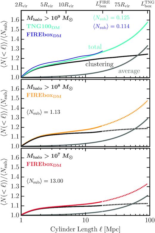
It is important to quantify the contribution of correlated clustering to counts for |$\ell \gt 2\, R_{\rm vir}$|, i.e. when subtracting off the contribution of subhaloes to N(< ℓ), what is the fractional contribution of the population of clustered haloes compared to the average halo population at |$\ell \gt 2\, R_{\rm vir}$|? This is explicitly address in Fig. 7, which shows the total average cumulative count of 109 M⊙ haloes in TNG100 for cylinder lengths ranging from the edge of the virial radius to the edge of the box. We plot the average count 〈N(< ℓ)〉 in units of the average cumulative count from subhaloes 〈Nsub〉 ≡ 〈N(ℓ < 2Rvir)〉, where 〈Nsub〉 = 0.072. The full count from the simulation (labelled as ‘total’) is shown by the magenta curve while cylinders that are assumed to have the average background outside of the virial radius (labelled ‘average’) are plotted as the light grey curve. To quantify the excess clustering associated beyond substructure, we take the difference between the magenta and grey curves. This results in the black curve (‘clustering’). The excess clustered contribution asymptotes to ∼1.35〈Nsub〉 at |$\ell \approx 70\ \mathrm{Mpc}\ ({\sim }75\, R_{\rm vir})$|. This means that local clustering boosts the expected signal by |$\sim 35{{\ \rm per\ cent}}$| compared to what we would expect from subhaloes alone. We show similar results for lower mass haloes in other simulations in Appendix B. Broadly speaking, the boost from local clustering is smaller relatively in DMO simulations that do not have enhanced subhalo destruction from the central galaxy. Note that the clustering contribution is larger than the average contribution out to |$\ell \approx 65\, {\rm Mpc}$|, or equivalently, |$\sim \! 130\, R_{\rm vir}$|.
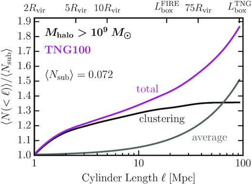
Boost in counts from local clustering: The mean count of LOS haloes more massive than 109 M⊙ within lens-centred cylinders from TNG100 relative to the mean count within the virial radius |$\langle N_{\rm sub} \rangle \equiv \langle N(\ell \lt 2\, R_{\rm vir})\rangle$| is presented here. The magenta line shows the mean total count from the simulation (labelled ‘total’), while the grey line shows counts in cylinders that assume the density of haloes matches the mean background (dubbed ‘average’) for |$\ell \gt 2\, R_{\rm vir}$|. The black line shows the difference between the ‘total’ and ‘average’ contributions; this is the component that is attributable to local halo clustering (dubbed ‘clustering’). We see that the local clustering effect provides a boost of |$\sim 35{{\ \rm per\ cent}}$| compared to the subhalo count alone and that this contribution dominates the ‘average’ contribution out to |$\sim \! 65\, {\rm Mpc} \approx 130\, R_{\rm vir}$|.
3.4 Structure along principal axes
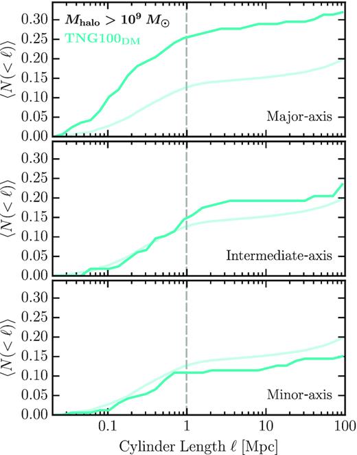
CDM haloes have significant triaxiality (e.g. Frenk et al. 1988; Dubinski & Carlberg 1991; Warren et al. 1992; Cole & Lacey 1996; Jing & Suto 2002; Bailin & Steinmetz 2005; Kasun & Evrard 2005; Allgood et al. 2006; Paz et al. 2006; Bett et al. 2007; Muñoz-Cuartas et al. 2011; Despali, Giocoli & Tormen 2014; Vega-Ferrero, Yepes & Gottlöber 2017; Lau et al. 2020), which could also mean that subhaloes are found preferentially along the host’s major (densest) axis (e.g. Zentner et al. 2005). This effect can qualitatively impact our analysis of lens-centred projections, especially for substructure lensing. Furthermore, it is likely that galaxy lenses are biased to be oriented with the LOS coinciding with the host halo’s major axis (Mandelbaum, van de Ven & Keeton 2009; Osato et al. 2018), as this configuration produces a larger surface mass density for a fixed overall mass distribution. In order to explore the potential magnitude of this effect, we calculate dark matter halo shapes from the lens targets using the shape inertia tensor as discussed in Allgood et al. (2006). We include all dark matter particles within a shell between |$10-20{{\ \rm per\ cent}}$| of Rvir as a conservative approach for our sample of haloes. Using a shell rather than the enclosed mass minimizes the influence of particles with radii smaller than the numerical convergence scale. The resulting eigenvalues of the shape tensor are proportional to the square root of the principal axes of the dark matter distribution. We then re-do the analysis of Section 3, now aligning the lens-centred projections along each principal axis of the lens–mass halo.
Fig. 8 plots the results for the average (mean) counts along each principal axis for haloes more massive than 109 M⊙ in TNG100 (for comparison with TNG100DM, see Fig. A2). The top, middle, and bottom panels depict the average counts along the major axis, intermediate axis, and minor axis, respectively, with cylinders of radius |$\mathcal {R} = 10\ \rm kpc$|. For comparison, the faded solid line in each panel shows the mean counts presented previously in Fig. 5. We see that the major axis sightline results in measurably more haloes, on average, than do other orientations. The boost along the major axis is |$\sim 30{{\ \rm per\ cent}}$| compared to the random LOS, with essentially the entire contribution coming from subhaloes (and backsplash haloes). Along the minor axis, on the other hand, average counts are significantly reduced. Projections along the intermediate axis are comparable to the average counts shown in Fig. 4. It is clear that lens-centred projections along the major or minor axis can non-trivially boost or decrease the lensing signals by a factor of ∼2. This factor is also acquired for analogue simulation neglecting the presence of the central galaxy and baryons (see Fig. A2).

Projections along the principal axes: Similar presentation as Fig. 4, but now filled solid lines show the counts for TNG100 haloes Mhalo > 109 M⊙ along the major, intermediate, and minor axis in the top, centre, and bottom panels, respectively. The transparent lines give the mean counts of the substructure with local clustering counts of TNG100 presented previously in Fig. 5. Sightlines oriented along the major (minor) axis of the halo result in a non-trivial increase (decrease) in the number of perturbers encountered along the sight line.
4 SUMMARY
Using the set of TNG100 and DMO FIREbox cosmological simulations, we quantify the effect of local clustering on gravitational lensing searches for low-mass dark matter haloes. We specifically focus on lens–mass haloes of mass Mvir ≃ 1013 M⊙ at z = 0.2 as prime targets for future lensing surveys and explore counts of haloes down to Mhalo = 107–9 M⊙.
Our primary result is that local clustering can boost the expected LOS perturber halo counts significantly compared subhaloes alone. The signal exceeds that expected for an average background projection to distances in excess of ±10 Mpc from the lens host (Fig. 4), with a significant excess within |$2-5\, R_{\rm vir}$|. We provide an analytic expression for this contribution (equation 3), which we hope will be useful in full lensing interpretation studies.
Using full-physics TNG100 simulations (which resolve haloes down to 109 M⊙), we find that the central galaxy in lens–mass hosts depletes subhaloes by |$\sim 70 {{\ \rm per\ cent}}$| compared to DMO simulations (see Fig. 5). This result agrees with previous studies (Despali & Vegetti 2017; Graus et al. 2018). From TNG100, the excess local clustering outside of the virial radius gives an expected count that is |$\sim 35{{\ \rm per\ cent}}$| higher than would be expected from subhaloes alone (Fig. 7).
Local contributions to perturber counts are also affected by halo orientation. The above results assume a random lens-orientation with respect to the observer, but if there is a bias for lenses to be oriented along the principal axis (e.g. Dietrich et al. 2014; Groener & Goldberg 2014), then the expected local count may be enhanced. Our initial exploration of this issue indicates that local projected counts are |$\sim 50{{\ \rm per\ cent}}$| higher when the target halo is oriented along the major axis compared to a random orientation (Fig. 8). This result, in turn, has implications for derived constraints on the mass spectrum of perturbers and accompanying constraints on dark matter particle properties.
The above results will be particularly important for low-redshift lenses (zl ∼ 0.2), such as those in the SLACS sample (Vegetti et al. 2014). For such lenses, Despali et al. (2018) find that subhaloes should contribute |$\sim 30-50{{\ \rm per\ cent}}$| of the total perturber signal relative to LOS haloes that neglect local clustering. With clustering included, the local (subhalo + clustering) contribution may well be comparable to |$\sim 67.5{{\ \rm per\ cent}}$| of the total LOS contribution that neglect clustering (or |$\sim 40{{\ \rm per\ cent}}$| of the total contribution) for some lenses, especially those with lower redshift sources (zs ∼ 0.6). Taking into account any biases in lens–halo orientation is also important for these lenses, as an additional |$\sim 50{{\ \rm per\ cent}}$| boost in counts from local clustering could significantly affect interpretations.
ACKNOWLEDGEMENTS
This article was worked to completion during the COVID-19 lockdown and would not have been possible without the labours of our essential workers. We thank Ran Li for helpful comments in improving the early version of this article. We are thankful to Quinn Minor and Manoj Kaplinghat for helpful discussions. The authors thank the Illustris collaboration for facilitating the IllustrisTNG simulations for public access and the FIRE collaboration for the use of the DMO FIREbox simulation for our analysis. AL and JSB were supported by the National Science Foundation (NSF) grant AST-1910965. AL was partially supported by NASA grant 80NSSSC20K1469. MBK acknowledges support from NSF CAREER award AST-1752913, NSF grant AST-1910346, NASA grant NNX17AG29G, and HST-AR-15006, HST-GO-14191, HST-GO-15658, HST-GO-15901, and HST-GO-15902 from the Space Telescope Science Institute, which is operated by AURA, Inc., under NASA contract NAS5-26555. RF acknowledges financial support from the Swiss National Science Foundation (grant no. 157591 and 194814). The analysis in this manuscript made extensive use of the python packages colossus (Diemer 2018), numpy (van der Walt, Colbert & Varoquaux 2011), scipy (Oliphant 2007), and matplotlib (Hunter 2007). We are thankful to the developers of these tools. This research has made all intensive use of NASA’s Astrophysics Data System (http://ui.adsabs.harvard.edu/) and the arXiv eprint service (http://arxiv.org).
DATA AVAILABILITY
The data supporting the plots within this article are available on reasonable request to the corresponding author. A public version of the arepo code is available at https://arepo-code.org/about-arepo. The IllustrisTNG data, including simulation snapshots and derived data products are publicly available at https://www.tng-project.org/. A public version of the gizmo code is available at http://www.tapir.caltech.edu/ phopkins/Site/GIZMO.html. Additional data from the FIRE project, including simulation snapshots, initial conditions, and derived data products, are available at https://fire.northwestern.edu/data/.
Footnotes
The Illustris data are publicly available at https://www.tng-project.org/
The FIRE project website: http://fire.northwestern.edu
The highest resolution box is actually TNG50-1, but was not publicly available by the time this article was submitted.
We have also experimented with higher unbound fractions of |$90{{\ \rm per\ cent}}$| and |$95{{\ \rm per\ cent}}$| with a fixed value of b = 0.20. We chose the unbound fraction of |$70{{\ \rm per\ cent}}$| and an fof linking of b = 0.20 because they provide the best match with TNG100DM catalogues for Mhalo > 109 M⊙.
A backsplash excess is also hinted at pictorially in Fig. 3 (top panel) from the magenta dots in the (edge-on) lens-centred projection
Recently, Kelley et al. (2019) presented high-resolution zoom simulations for MW–mass DMO haloes while accounting for the central galaxy and found that the depletion of substructure is about roughly the same factor for haloes down to 107 M⊙ at z = 0. While we are drawing possible conclusions from MW–mass haloes, this scaling could translate to our lens–mass haloes.
REFERENCES
APPENDIX A: COUNTING STATISTICS
A1 Sampling variance
In Section 3.1, we discussed the possibility that the differences in local clustering signal between TNG100DM and FIREboxDM could arise from sampling variance – there are only three lens–mass hosts in FIREboxDM – rather than differences in large-scale structure (compare the red and cyan curve in Fig. 4). In order to explore this more fully, Fig. A1 shows |$\langle \mathrm{d} N/ \mathrm{d} \ell \rangle$| for TNG100DM (cyan) and FIREboxDM (red). This figure mirrors Fig. 4 except now we are using a cylinder radius with the size of the lens–mass virial radius (|$\mathcal {R} = R_{\rm vir}\simeq 500$| kpc) as opposed to the typical Einstein radius (|$\mathcal {R} = 10$| kpc) in order to improve counting statistics. The solid lines depict the mean of all projections while the dashed (shown only for TNG100DM) is the median of all projections. The cyan band encloses the ±1σ of all of the individual curves around median.
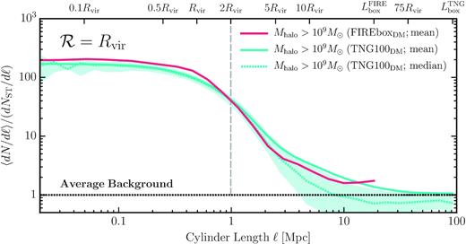
Analogous to Fig. 4, now with results of TNG100DM (cyan) and FIREboxDM (red) for Mhalo > 109 M⊙ for cylinders with a radius size comparable to the lens mass halo (|$\mathcal {R} = R_{\rm vir}$|) as opposed to the lens halo’s Einstein radius (|$\mathcal {R} = 10\, {\rm kpc}$|). The solid curves depict the mean differential count while the dashed cyan is the median differential count for TNG100DM. The cyan band encloses the ±1σ region of the curves. The median counts fall below the mean counts, indicating that the mean counts are strongly affected by rare, high-count orientations.
For ℓ < 1 Mpc, the median and mean curve for TNG100DM are consistent with one another, but for ℓ > 1 Mpc we see that the average count (which is what we plot in Fig. 4) sits well above the median. This is indicative of a highly non-Gaussian distribution, with a tail skewed towards large fluctuations, as expected for non-linear dark matter structure. Specifically, rare (high-count) events drive the average higher than the median. If this is the case, we require a large number of realizations in order to sample enough of the distribution to capture the true average. As further evidence that sample variance is the cause of the differences in local clustering signal between TNG100DM and FIREboxDM, the median line in Fig. A1 falls below the average background (black dashed) at ℓ ≈ 10 Mpc. This is due to a large number of null counts.
Though the average count from FIREboxDM falls below the average line from TNG100DM, we see that it falls within the 1σ band about the median. Given that we only have three host haloes in our sample, this would not be unexpected even if the haloes were sampling the same large-scale structure field. Naively, there is a |$\sim 30 {{\ \rm per\ cent}}$| chance that three randomly drawn distributions will lie within 1σ of the median. Given that we only have three host haloes, we conclude that the observed result is consistent with small-number statistics.
A2 Choice of cylinder radius
The conclusions made in the main text are based on the average number density of subhaloes within a project cylinder radius of 10 kpc, which is comparable to the typical Einstein ring of our 1013 M⊙ lens–mass haloes. The choice of |$\mathcal {R}=10\rm \, kpc$| could bias our results towards higher substructure, and potentially, LOS halo counts, as massive galaxy lenses typically have Einstein ring radii of ∼5 kpc (Bolton et al. 2008).
In Fig. A2, we demonstrate how the selection of smaller lens radii does not impact the trends discussed in our main analysis. Both the top and bottom plot mirrors exactly Fig. 4, now with the top and bottom plot showing results for a projected radius of 5 and 2 kpc, respectively. We find that we are able to mostly recover the same trend seen for the 10 kpc projected radius from Fig. 4 for both |$\mathcal {R}=$| 5 and 2 kpc. In the 5 kpc radius projection, the curves are more noisier than the 10 kpc owing to the increasing fraction of projections with zero haloes. We would argue that the |$\mathcal {R}=5$| kpc size projections have comparable trends to the |$\mathcal {R}=10$| kpc case. Out to ℓ = 5Rvir, most of the mean differentials drives faster down to the average compared to the 10 kpc case, but we suspect this is owed to low number statistics along with the sampling variance for TNG100DM (see discussion in Appendix A1). This becomes more apparent for the smaller projected radius of 2 kpc, as the fraction of projections of zero haloes increases appreciably. Note that the Mhalo >109 M⊙ result is impacted greatly by sampling variance the low number of haloes along the LOS.
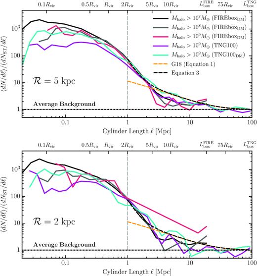
Analogous to Fig. 4, now for cylinders with a radius size |$\mathcal {R} = 5$| kpc and a much smaller annulus |$\mathcal {R} = 2$| kpc. While the curves are much noisier as the radius size becomes smaller (owing to the increased fraction of null sightlines), we are able to recover the same trend for the differential counts seen for a projected radius of |$\mathcal {R} = 10$| kpc.
APPENDIX B: SUPPLEMENTARY DISCUSSION WITH DARK MATTER ONLY PHYSICS
This appendix presents the DMO results from TNG100DM and for FIREboxDM and provides additional elaboration of the results in the main text. Section B1 picks up from later discussion of Section 3.3 and Section B2 picks up from Section 3.4.
B1 Clustering contribution to the line-of-sight population
Fig. B1 presents the contribution of the simulated clustering to the LOS halo population in TNG100DM and FIREboxDM. Namely, the top, middle, and bottom panels plots the subhalo populations based on the lower mass cuts of 109 M⊙, 108 M⊙, and 107 M⊙, respectively. The coloured curves, labelled ‘total’, are the actual results of the simulation out to the box using our method discussed in the main text. The average background expectation for haloes above the low-mass cuts in each panel is depicted by the grey curves. The clustering contribution from the simulations, labelled ‘clustering’, are plotted as the black curves, which is the difference between the ‘total’ curve and ‘average’ curves. Like before, all results are normalized by the 〈Nsub〉 quantified from out lens–mass sample. Since the actual FIREboxDM results extend out to |$L_{\rm box}^{\rm FIRE}$|, we extrapolate the curves out to |$L_{\rm box}^{\rm TNG}$|using equation (1) (using equation 3 is also equally adequate).
Like Fig. 7, now showing only the results for TNG100DM and FIREboxDM. In the top panel, the black and grey curve are computed based off of the total counts from TNG100DM (cyan curve). As a comparison, the blue curve shows the total counts from FIREboxDM out to |$L^{\rm FIRE}_{\rm box}$|. The middle and bottom panel are presented similarly with their curves extrapolated out to the |$L^{\rm TNG}_{\rm box}$| using equation (3).
Starting with the counts 109 M⊙ (top panel), clustering acts as the most contributing component to the LOS halo population until the average background takes over at ℓ ≈ 75Rvir (or |$r\approx 37.5\ \rm Mpc$|) for TNG100DM (cyan curve). As a comparison check, we plotted the FIREboxDM results of 109 M⊙ (thin blue curve) and find minimal difference in results. Note the clustering component is determined from TNG100DM and not FIREboxDM. The clustering component in TNG100DM boosts about 1.5〈Nsub〉 out until the average background takes over at |$\ell \approx 70\ \rm Mpc$| (or r ≈ 35 Mpc). This is less significant than the TNG100 in the main text, the clustering component strongly boosts the number of LOS haloes to about 1.7〈Nsub〉 until the average background takes over.
As we go further down to the low-mass cuts of the subhalo populations, the contribution from correlated clustering becomes much weaker for decrease mass. For |$M_{\rm halo} \gt 10^{8}\ \rm M_{\odot }$| (middle panel), the clustering component boosts the number of LOS haloes to only about ∼1.2〈Nsub〉 until the average background takes over at about |$\ell \approx 60\ \rm Mpc$| (or r ≈ 30 Mpc). The clustering component for |$M_{\rm halo} \gt 10^{7}\ \rm M_{\odot }$| (bottom panel) becomes weaker by only boosting the number of LOS haloes to only about ∼1.1〈Nsub〉 until the average background takes over at r ≈ 30 Mpc). In order to conclude with more robust predictions, a larger sample lens–mass haloes in comparable cosmological environments is needed to reduced the uncertainty possibly found in 〈Nsub〉 for these low-mass haloes.
B2 Structure along principal axes
Fig. B2 plots the mean subhalo counts as seen from lens-centred projections along the principal axis of the TNG100DM lens–mass haloes. The axes were computed using the method detailed in Section 3.4. Shown are only the results from TNG100DM since these cosmological volumes have enough lens-centred mass haloes to provide enough statistics since each halo has only three principal axis to orientate on. Moreover, FIREboxDM, while useful for simulating 107–8 M⊙ haloes in cosmological environment, has only three lens-centred hosts, which will not provide adequate statistics to present. Though, we find similar trends. The top, middle, and bottom panels depict the average counts along the major-, intermediate-, and minor-axis, respectively. For comparison, the faded solid line in each panel plots the mean counts presented previously in Fig. 5. We again see that projections along the major axis of DMO lens–mass haloes, subhaloes tend to populate on the densest principal axis. This effect is more dramatic for the substructure compared to the TNG100 shown previously, owing to the lack of a central galaxy.
Like Fig. 8, but now showing the TNG100DM counts for haloes Mhalo > 109 M⊙ along the major, intermediate, and minor axis in the top, centre, and bottom panels, respectively. Plotted for comparison, the transparent lines are the mean counts of the substructure with local clustering counts for TNG100DM presented previously in Fig. 5.
Projections size of the Einstein radius along the major axis find around |$75{{\ \rm per\ cent}}$| of the projections to contain no substructure out to the size of the halo. Along the minor axis, this is around |$\sim 90{{\ \rm per\ cent}}$|. Additionally, the substructure counts appear to be almost comparable to the mean from Fig. 4, though slightly less. Done on the intermediate-axis, this results in counts somewhat comparable to the mean counts, though we see |$\sim \! 5{{\ \rm per\ cent}}$| boost in the LOS component.
APPENDIX C: COMPARISON BETWEEN MASS FUNCTIONS OF LENS–MASS SAMPLE
As mentioned in Section 2, the rockstar halo finder was ran for the TNG suites while rockstar was applied to FIREboxDM. Fig. 1 provides confidence in the resulting halo catalogues used in the main text, as both catalogues show robust agreement with the analytical prediction. However, halo finders vary in routines for quantifying the masses for subhaloes and can potentially produce different mass functions when ran to the same simulations. It would be worth comparing our resulting halo finders with one another based on the resolved substructure population found for our lens-target haloes at z = 0.2.
Fig. C1 shows the subhalo mass functions for the 1013 M⊙ target-lens systems in TNG100DM (purple) while the three from FIREboxDM (black curves). The purple band for TNG100DM encloses the |$90{{\ \rm per\ cent}}$| dispersion of all of the target-lens subhalo mass functions. Significant disagreement could arise based on the assignment of particles to subhaloes from halo finders (Graus et al. 2018). To clarify this point, Fig. C2 provides a different view of subhalo sample, where the subhalo Vmax function for the same lens–target systems.
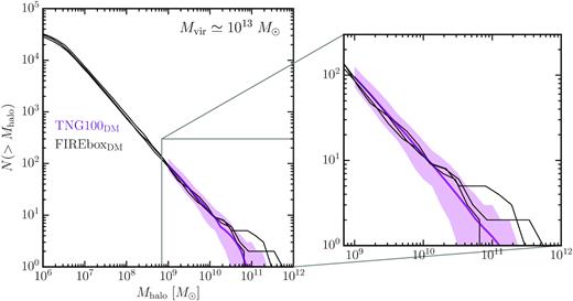
The subhalo mass functions for the lens-target haloes in our main sample compared between the TNG100DM (purple curve) and FIREboxDM (black curves). FIREboxDM follows the median TNG100DM curves sufficiently for the subhalo masses ranging from ∼109–10 M⊙ while the three lens-target in FIREboxDM hosts several more massive 1011 M⊙. Though, the curves are still mostly found enclosed in the |$90{{\ \rm per\ cent}}$| dispersion. The agreement depicted from the subhalo mass functions provides further justification for the choice of our rockstar parameters detailed in Section 2.

The subhalo Vmax functions for the lens-target haloes in our main sample compared between the TNG100DM (purple curve) and FIREboxDM (black curves).
