


ABSTRACT
We study systematic effects from half-wave plates (HWPs) for cosmic microwave background (CMB) experiments using full-sky time-domain beam convolution simulations. Using an optical model for a fiducial spaceborne two-lens refractor telescope, we investigate how different HWP configurations optimized for dichroic detectors centred at 95 and 150 GHz impact the reconstruction of primordial B-mode polarization. We pay particular attention to possible biases arising from the interaction of frequency-dependent HWP non-idealities with polarized Galactic dust emission and the interaction between the HWP and the instrumental beam. To produce these simulations, we have extended the capabilities of the publicly available beamconv code. To our knowledge, we produce the first time-domain simulations that include both HWP non-idealities and realistic full-sky beam convolution. Our analysis shows how certain achromatic HWP configurations produce significant systematic polarization angle offsets that vary for sky components with different frequency dependence. Our analysis also demonstrates that once we account for interactions with HWPs, realistic beam models with non-negligible cross-polarization and sidelobes will cause significant B-mode residuals that will have to be extensively modelled in some cases.
1 INTRODUCTION
The measured temperature anisotropies of the cosmic microwave background (CMB) provide a large part of the empirical basis for ΛCDM, the current standard model of cosmology (MacTavish et al. 2006; Bennett et al. 2013; Planck Collaboration VI 2020a). Additional cosmological information from the CMB will mainly come from accurate characterization of the polarized component of the anisotropies. Although many cosmological constraints will benefit from polarization measurements (Galli et al. 2014), the most notable advance is perhaps seen in the search for primordial gravitational waves, which might have a distinctive signature in the B-mode component of the CMB polarization (Kamionkowski, Kosowsky & Stebbins 1997; Zaldarriaga & Seljak 1997).
Experiments have to minimize spurious polarization in order to measure the weak CMB polarization. An attractive approach is the use of a half-wave plate (HWP): a birefringent optical element that shifts the polarization angle of linearly polarized light that passes through. The shift depends on the orientation of the plate, which allows modulation of the polarized sky signal by rotation of the HWP. An ideal rotating HWP only modulates the linearly polarized sky signal and therefore allows one to cleanly separate this desired signal from unpolarized sky signal. Unfortunately, non-ideal HWPs impede perfectly controlled modulation and indirectly cause spurious polarized signal of their own. The merit of an HWP has to be carefully weighed against the downsides.
Multiple polarimetric experiments have employed HWPs. Examples include MAXIPOL (Johnson et al. 2007); POLARBEAR (The Polarbear Collaboration 2010; Hill et al. 2016); ABS (Kusaka et al. 2014); SPIDER (Rahlin et al. 2014); PILOT (Misawa et al. 2014); BLAST (Galitzki et al. 2016); and EBEX (Aboobaker et al. 2018). In addition, several upcoming B-mode experiments are planning to use HWPs; see e.g. the Simons Observatory small-aperture telescopes (Galitzki et al. 2018) and the proposed LiteBIRD satellite (Suzuki et al. 2018; Sugai et al. 2020). Consequently, there exists a rich body of literature describing the optical impact of HWPs, including descriptions of various HWP non-idealities (Bryan et al. 2010b; Kusaka et al. 2014; Pisano et al. 2014; CMB-S4 Collaboration 2017) and mitigation strategies (Bao et al. 2012; Matsumura 2014; Bao et al. 2016; Vergès, Errard & Stompor 2020).
In order to separate astrophysical foregrounds from the CMB signal, experiments observe in several frequency bands. For example, the proposed LiteBIRD satellite effort currently proposes to deploy 15 frequency bands in three telescope modules spanning 34–448 GHz (Suzuki et al. 2018; Sugai et al. 2020). Successful implementation of wide-band polarization modulation is arguably quite technically challenging: the modulation efficiency of simple birefringent crystals is constant over a relatively small frequency range and the plate will cause loss in linear polarization for signals outside that frequency range. In order to efficiently modulate polarization over a wide frequency range, for example, to support the use of dichroic or even trichroic bolometers (Suzuki et al. 2014), an achromatic half-wave plate (AHWP) is likely required (Hill et al. 2016; Komatsu et al. 2018). AHWPs largely remove the frequency-dependent loss in polarization modulation efficiency, but they can also rotate the polarization angle of linearly polarized light by a frequency-dependent angle. This angle offset, which can be significant for certain AHWP configurations, is potentially troublesome. When present, an observer needs prior knowledge of the spatial and spectral energy distribution (SED) of various astrophysical sources in order to correctly interpret the modulated sky signal. For instance, a sky region dominated by polarized dust requires a different angle correction compared to one dominated by the polarized CMB (Bao et al. 2012; Abitbol et al. 2020).
In this paper, we investigate how non-idealities from a collection of (A)HWP configurations optimized for dichroic detectors sensitive to both 95 and 150 GHz limit our ability to reconstruct primordial B-mode polarization. We pay particular attention to the frequency-dependent polarization rotation angle for these different configurations. It has been pointed out, see e.g. Vergès et al. (2020), that such angle offsets will inevitably lead to biased sky maps that require different correcting polarization angles for each sky component. Here, we provide a realistic example of this effect to judge its importance. We also simulate the interaction between the HWP non-idealities and a realistic polarized beam and point out the importance of this potential systematic. To produce these simulations, we extend the beamconv 1 code, first described in Duivenvoorden, Gudmundsson & Rahlin (2019). The new code allows us to simulate the effects of non-ideal HWPs on the time-ordered data (TOD) of CMB experiments. To our knowledge, this is the first time that a publicly available code can perform realistic time-domain simulations that include both HWP non-idealities and all-sky beam convolution with asymmetric beams.
This paper is organized as follows: in Section 2, we introduce the mathematical framework and the data model used for the simulations. The description of our fiducial instrument, the HWP properties, the proposed scanning strategy, and the input sky models are presented in Section 3. Results are given in Section 4. We discuss the results and formulate our conclusions in Section 5.
2 MATHEMATICAL FRAMEWORK
In this section, we derive a data model for a typical CMB polarization experiment (see Section 2.2). The model describes the effects of a non-ideal HWP combined with beam convolution on the TOD. We generalize the model presented in Bryan et al. (2010b) to multilayer HWPs and arbitrary shaped and non-trivially polarized beams. First, however, we briefly discuss the Mueller matrix description of an HWP. See Hecht (2002) or Gil Pérez & Ossikovski (2016) for general introductions to the Mueller matrix formalism and Bryan, Montroy & Ruhl (2010a), Essinger-Hileman (2013), Moncelsi et al. (2014), Salatino, de Bernardis & Masi (2017), and Salatino et al. (2018) for applications to HWPs for CMB experiments.
Throughout this section, we make use of the Einstein summation convention: pairs of upper and lower indices are implicitly summed over. We use θ and ϕ to denote the polar and azimuthal angles of the standard spherical coordinate system. The metric of the sphere is given by gij = diag(1, sin 2θ) in these coordinates.
2.1 Half-wave plate Mueller matrix
Mueller matrices describe the set of linear transformations that transform Stokes vectors to other valid Stokes vectors. Linear optical media such as HWPs is described by Mueller matrices. Multiplying a Stokes vector by such a Mueller matrix describes how the HWP alters the polarization properties of the radiation described by the Stokes vector.
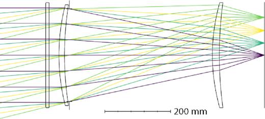
Sketch of telescope model used for this study. Light coming in from the left interacts with an HWP before hitting the primary lens. Light from the primary lens then gets further focused by the secondary lens before hitting the focal plane (on the right). The edge pixel has a beam centroid of 14° relative to boresight (see ray bundle emitted from top right corner).
Pancharatnam (1955) showed that there exist combinations of layers of birefringent materials that, unlike the single-layer HWPs, can behave in an almost achromatic manner. The resulting AHWPs have a low frequency dependence in polarization modulation efficiency across a broad frequency range. This is achieved by introducing a relative rotation angle for one or several of the birefringent layers such that not all of the fast optical axes are aligned. The set-up is discussed in detail in Title (1975). A complication of AHWPs is their effective frequency-dependent rotation angle offset. We will come back to this issue in Section 3.4.
The Mueller matrix of an AHWP, being composed of more than one birefringent layer, cannot be adequately described by the four parameters in equation (3). Instead, the transfer matrix method (TMM) can be used to generate an appropriate Mueller matrix. The TMM formalism captures the response of materials that are composed of any collection of dielectric and birefringent media. For the work presented here, we use the publicly available code described in Essinger-Hileman (2013) to calculate the Mueller matrices of the HWPs that we study.2
2.2 Data model
Fig. 2 helps to qualify the rather verbose expressions for the above harmonic coefficients. It illustrates the effect of a non-ideal HWP on the TOD by comparing the corresponding power spectrum densities for two cases: without an HWP and with a non-ideal HWP (see Section 3.3). Recall that ideal HWP modulation will only modulate the Q and U sky signal, which it will do at a modulation frequency 4να, where να is the HWP rotation frequency. It can be seen that the non-ideal HWP introduces an additional spurious 2να modulation of the I sky (second line of equation 15), a 2να modulation of the Q and U sky (first and second line of equation 16), and a 2να modulation of the V sky (second line of equation 17, not shown in the figure). Finally, the non-ideal HWP also introduces a spurious constant 0να modulation of the Q and U sky (fourth line of equation 16). Note that Fig. 2 omits the case of an input V sky. The να dependence of the V-input case will be the same, qualitatively, as the Stokes I-input case.
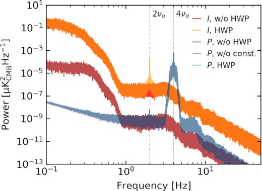
Power spectral densities (PSDs) corresponding to a typical 2-h segment of noiseless TOD for a single detector. The curves labelled I (P) correspond to scans over an I-only ((Q, U)-only) simulated CMB sky. The curves labelled HWP include HWP modulation using the three-layer BR3 HWP configuration (to be discussed in Section 3) spinning at a frequency να of 1 Hz. The curve labelled P, w/o const. (overlapping with P, HWP but slightly different below |$\sim {2}{\, \mathrm{Hz}}$|) incorporates the same HWP modulation, but does not include the HWP systematic that is constant with HWP angle α, see equation (16). The curves labelled w/o HWP do not include HWP modulation. The simulated data are recorded at a monochromatic frequency of 90 GHz using a Gaussian beam with a full width at half-maximum of 32.2 arcmin. Each curve is the average of 10 PSDs corresponding to successive 2-h scans. The scan strategy is described in Section 3.1.
The dependence on HWP angle α of the different terms in the data model is relevant because this dependence is used by the subsequent map-making procedure to distinguish between I, Q, U, (and possibly V) sky signal. Leakage between the Stokes parameters will occur when the data model used by the map maker does not capture the full α modulation of the TOD. For the experimental configuration considered in this work, see Section 3, we find that the I → (Q, U) leakage that is caused by ignoring the 2να terms during map making is subdominant to the Q↔U leakage that is caused by ignoring non-idealities in the 4να term.
The data model described by equations (11)–(21) is now implemented in the beamconv library. The frequency dependence of the model is handled by approximating the integral over the instrumental frequency band with a small number (nν = 7 for the results in Section 4) of monochromatic input skies, beams, and HWP Mueller matrices. The memory costs and computational scaling of the algorithm have thus gained a linear scaling with nν compared to the algorithm in Duivenvoorden et al. (2019) but are unchanged otherwise. The algorithm allows for efficient time-domain simulations that include all-sky beam convolution with asymmetric beams and non-ideal HWPs.
3 SIMULATION SET-UP
We consider a telescope similar to the one described in Duivenvoorden et al. (2019), but with an HWP in front of the primary lens. Incoming radiation passes through the HWP followed by a pair of lenses before being absorbed by the detectors on the focal plane (see Fig. 1). A beam profile for a typical 150-GHz detector used in this analysis is shown in Fig. 3. We model 50 dichroic detectors sensitive to two 30-GHz-wide frequency windows centred at 95 and 150 GHz. The detectors are evenly distributed on a square grid of a focal plane fed by a 30- cm aperture telescope. The field of view of this square grid is only 7° compared to the 28° that can be supported by this telescope; the detectors therefore only cover a fraction of the focal plane. The spectral response of the detectors is assumed to be represented by a top-hat function within each band. In order to test frequency-dependent effects, we run simulations at seven subfrequencies within a band. These subfrequencies are 80, 85, 90, 95, 100, 105, and 110 GHz for the 95-GHz band and 135, 140, 145, 150, 155, 160, and 165 GHz for the 150-GHz band (see hatched regions in Fig. 4).
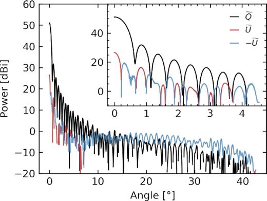
Azimuthally averaged beam profiles (dBi units) for a representative detector of one of the 50 used in this analysis. Shown are the Stokes |$\widetilde{Q}$| and |$\widetilde{U}$| beam components. For this figure, we have defined the Stokes parameters with respect to the Ludwig-3 basis (Ludwig 1973). This basis is approximately Cartesian around the beam centre and has been aligned with the polarized element of the detector. As a result, the |$\pm \widetilde{U}$| profile quantifies the amount of non-aligned (or ‘cross-polar’) polarized sensitivity of the beam. It can be seen that |$|\widetilde{U}|$| is subdominant close to the centre of the beam (see inset) while having a relatively large contribution at large opening angles.
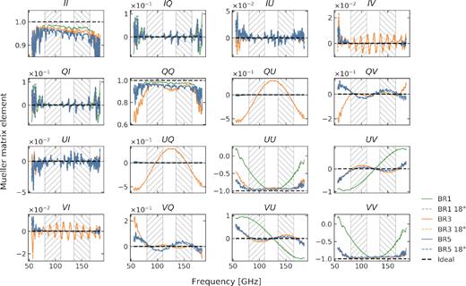
HWP Mueller matrix elements as a function of frequency in the normal incidence case (solid lines) and for an incidence angle ϑinc of 18° (dashed lines, virtually indistinguishable from solid lines) simulated using the TMM. The three HWP configurations described in Table 1 are shown. A 31.4° HWP rotation angle offset is applied to the three-layer BR3 model. The black dashed line represents the ideal HWP (T = −c = 1, ρ = s = 0 in equation 3). The grey hatched bands illustrate the two instrumental frequency bands used in this work.
3.1 Simulated scanning
Using the updated version of beamconv, we simulate 1 yr of satellite scanning for 50 detectors. We use a similar scan strategy as in Duivenvoorden et al. (2019), which is based on Gorski (2008) and Wallis et al. (2017). The satellite spins around its principal axis with a period of 600 s. It precesses about the boresight axis with a period of 90 min. The two axes are separated by 50°. We set the HWP rotation frequency να to 1 Hz (angular frequency of |${2 \pi }{\, \mathrm{rad\, s}^{-1}}$|) and sample the data at 12.01 Hz. Although the sampling frequency is likely an order of magnitude below that of a real experiment, we find that this rate suffices for our noiseless simulations. The resulting angular coverage is excellent and allows for simultaneous per-pixel recovery of I, Q, and U over the full sky. Even without a continuously spinning HWP, the average condition number of the per-pixel (I, Q, U) covariance matrix, which is inverted as part of the solution (Duivenvoorden et al. 2019), is approximately 2.9 for a Nside = 256 map. In comparison, the condition number approaches 2.0 (the minimum value) for all pixels when the HWP is spun with a 1-Hz rotation frequency.
3.2 Input maps
d0 uses a fixed spectral index (β = 1.54), a fixed temperature (|$T={20}{\, \mathrm{K}}$|), and the Commander dust template from Planck Collaboration IX (2016a) for AQ/U.
d1 extends the d0 model with spatially varying spectral index and temperature that are both given by the Commander templates from Planck Collaboration IX (2016a).
d2 modifies the d1 model with a spectra index that varies randomly on degree scales, following a Gaussian distribution: |$\beta \sim \mathcal {N}(\mu =1.59, \sigma ^2 = 0.04)$|.
d3 is the same as d2 except that |$\beta \sim \mathcal {N}(\mu =1.59, \sigma ^2 = 0.09)$|.
d4 models two dust populations as two modified blackbodies with different but spatially constant spectral indices and two different spatially varying temperatures and dust amplitudes (Meisner & Finkbeiner 2015).
d5 is a more physically motivated model based on the physical properties of two populations of dust grains (silicate and carbonaceous) (Hensley 2015; Hensley & Bull 2018).
The inclusion of these six models in our analysis serves to roughly bracket the current uncertainty in dust modelling. We note that the d3 model is designed to match the largest variation in spectral index allowed by the Planck data. We study the interplay between the HWP non-idealities and these different foreground models in Section 4.3.
3.3 Selection of HWPs
A wide range of HWP designs have been described and studied in the literature (Bryan et al. 2010b; The Polarbear Collaboration 2010; Hill et al. 2016; Aboobaker et al. 2018; Komatsu et al. 2018). HWP design involves a complex optimization problem where absorptive and reflective losses from materials with high index of refraction need to be balanced against the desire for unity polarization efficiency across a wide band. We choose to study three HWP configurations, which are loosely based on Bryan et al. (2010b) as a model of a one layer HWP, (Hill et al. 2016) for the three-layer HWP, and a five-layer HWP model taken from Komatsu et al. (2020). Some key properties of these three HWP configurations, which we denote as BR1, BR3, and BR5, are shown in Table 1.
HWP configurations adopted for the analysis presented in this paper. Orientation angles are those of the fast axis of the birefringent layers relative to the plane of incoming vertically polarized radiation. The rotation angle offset is given in each band following equation (24), for CMB and dust weights as defined in equation (25).
| Model | Orientation | Phase 95 GHz | Phase 150 GHz |
|---|---|---|---|
| CMB/dust | CMB/dust | ||
| BR1 | 0° | 0°/0° | 0°/0° |
| BR3 | {0°, 54°, 0°} | 30.75° / 31.16° | 32.51° / 32.30° |
| BR5 | {22.9°, −50°, 0° | ||
| 50°, −22.9°} | 0°/0° | 0°/0° |
| Model | Orientation | Phase 95 GHz | Phase 150 GHz |
|---|---|---|---|
| CMB/dust | CMB/dust | ||
| BR1 | 0° | 0°/0° | 0°/0° |
| BR3 | {0°, 54°, 0°} | 30.75° / 31.16° | 32.51° / 32.30° |
| BR5 | {22.9°, −50°, 0° | ||
| 50°, −22.9°} | 0°/0° | 0°/0° |
We adopt a fixed thickness, |$d={3.75}{\, \mathrm{mm}}$|, for the individual sapphire plate layers for all three polarization modulators. This thickness was found using the traditional formula for HWPs made of a single layer of birefringent material d = c/[2ν(ne − no)], where no and ne correspond to the index of refraction for the ordinary and extraordinary axes, respectively. The selected thickness is optimal for |$\nu = {126}{\, \mathrm{GHz}}$|, near the average of our two band centres. We adopt an antireflection coating similar to the one described in Coughlin et al. (2018) that is optimized for 75–170 GHz. We settle on three AR layers with thicknesses |$d_\mathrm{AR} = 0.5, 0.31, {0.257}{\, \mathrm{mm}}$| and individual indices nAR = (1.268, 1.979, 2.855). The above parameters are used as input to the TMM formalism to calculate the Mueller matrices of the HWPs. We produce a unique set of Mueller matrices for each unique HWP incidence angle ϑinc.
Fig. 4 shows the Mueller matrix elements for our three HWP configurations as function of frequency. It can be seen that the additional layers of the BR3 and BR5 HWPs improve the frequency uniformity of the polarization efficiency (see the UU elements) compared to the BR1 case. Describing the efficiency loss for the different Stokes parameters is a rather complicated task. Although the efficiency loss of Stokes I is easy to understand, as the II elements decrease in value with additional layers, the same is not true for the polarization efficiency.6 Because of these complications, we do not directly use the HWP Mueller matrix elements to correct our results for the efficiency loss. As will be detailed in Section 4, we settle for a more robust and simpler power spectrum based calibration method. Such an approach will likely also be taken by a real experiment. Finally, we note that the Mueller matrix models that we use do not include systematic effects caused by non-ideal manufacturing or material non-uniformity, which are likely to exist at some non-negligible level even in next-generation experiments.
3.4 Determining the AHWP induced rotation offset
AHWPs, such as the three- and five-layer configurations discussed in this paper, tend to have higher polarization efficiency over a given frequency range compared to a single-layer HWP. However, they also introduce an undesirable frequency-dependent phase between the in-going and out-going electric field that manifests itself as a frequency-dependent HWP rotation angle offset. Fig. 5 shows our HWP Mueller matrices, integrated over the two frequency bands, as a function of the HWP angle α. From the inner two-by-two set of panels it is clear that the three-layer HWP has a relatively large rotation angle offset. It turns out that the offset angle of the three-layer model also displays the largest variation with frequency. While the average value of this offset angle can be simply calibrated out, this large variation with frequency poses a difficulty: sky components with different frequency characteristics will require different offset angles after integration over the instrumental frequency band.
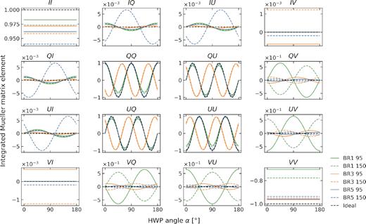
Mueller matrix elements for the three HWP models described in Table 1, integrated over the instrumental frequency bands (95: solid lines, 80–110 GHz; 150: dashed lines, 135–165 GHz) as a function of the HWP rotation angle. The dashed black lines represent the behaviour of the ideal HWP (T = −c = 1, ρ = s = 0 in equation 3). It can be seen that the BR3 configuration (orange lines) is out of phase with the other HWP configurations.
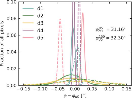
Distribution of optimal BR3 HWP rotation angle offset φ in the 95 GHz (solid lines) and 150 GHz (dashed lines) bands for the pysm Galactic dust models based on their per-pixel spectral energy distribution at Nside = 512. The distributions are given for the 40 per cent sky mask used in our analysis. The abscissa is expressed as the difference between the rotation angle offset φ and the reference angle φd0 corresponding to a modified blackbody with |$T={20}{\, \mathrm{K}}$| and β = 1.54 as in Table 1.
4 ANALYSIS RESULTS
For every simulated systematic effect, the same simulation is performed using an ideal HWP (T = −c = 1, ρ = s = 0 in equation 3). With ideal and non-ideal maps in hand, we can calculate difference maps that quantify signal residuals due to HWP-related systematics. The resulting difference maps cover the entire sky, but we use a 40 per cent sky mask (gal040; Planck Collaboration IX 2016a) before calculating power spectra using polspice (Challinor et al. 2011).
4.1 Calibration
Finally, we divide out a beam window function to correct the power spectrum for the azimuthally symmetric part of the beam. This allows us to directly compare the residual to theory spectra. For each simulation, we use a window function that corresponds to the averaged symmetric part of the input detector beams.
4.2 Scanning with an ideal Gaussian beam
We start by exploring effects that are purely caused by non-ideal HWPs. This is achieved by choosing a copolar polarized and azimuthally symmetric Gaussian beam model, see e.g. Duivenvoorden et al. (2019). Using this beam, we scan the CMB with the different HWP configurations; we summarize our results in Fig. 7. We find that only the BR3 configuration shows an appreciable B-mode residual in this case. All three HWP configurations outperform the case without HWP modulation, which shows a relatively large white-noise spectrum caused by small conditioning problems in the map-making solution that are approximately uncorrelated between pixels. It is instructive to determine which terms of the data model in equations (15)–(17) are causing the BR3 residual. It turns out that this spurious signal is due to E → B leakage from the 4να terms, i.e. non-idealities in the inner two-by-two part of the HWP Mueller matrix. We have checked that the residual is not caused by I → (Q, U) leakage due to the 2να term in equation (15) that couples the linearly polarized beam to the I sky signal: we obtain virtually identical residuals when the input Stokes I signal is artificially set to zero. The insignificance of the 2να term can be attributed to the smallness of the IQ and IU elements in the HWP Mueller matrices (see Fig. 5), the lack of a strong atmospheric I signal, and most importantly, the rather good conditioning of the map-making solution. Even without modification, the map maker corresponding to equation (27) accurately distinguishes between time-ordered signal that is modulated at 2να and 4να.
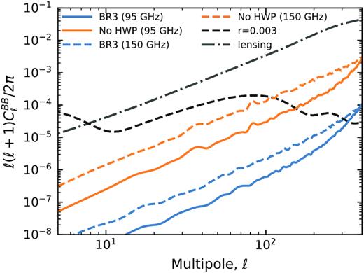
Residual B-mode power spectra obtained by observing the CMB with the BR3 configurations presented in Table 1 (including the rotation angle offset optimized for the CMB). The beams are Gaussian. We omit the BR1 and BR5 HWP configurations since their residuals fall below the limits on the vertical axis. The no-HWP case is also shown (orange curves).
Using the same set-up, we then explore the addition of a foreground component. Specifically, we simulate what happens when a map maker that uses an HWP angle offset φ (see equation 27) that is optimized for the CMB encounters polarized signal from Galactic dust. Fig. 8 shows the B-mode residual for this hypothetical situation as well as for the opposite case in which the CMB is observed with φ optimized for the SED of dust. We again only show the BR3 HWP configuration. The error in φ causes E → B leakage: the residual clearly traces the shape of the input E-mode spectrum. The effect is identical to that of a systematic polarization angle calibration error. It can be seen that for both cases the residual is larger for 95 GHz than for 150 GHz. This is due to the fact that the optimal BR3 offset angle for dust in the 95 GHz band differs from the optimal angle offset for the CMB by about 0.4° while the difference at 150 GHz is only half that.
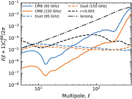
Residual B-mode power spectra generated when the CMB is observed using the BR3 HWP with a rotation angle offset optimized for the pysm Galactic dust model d1 (solid curves) and vice versa (dashed curves).
From this section it becomes clear that in the presence of multiple sky components a single HWP offset angle φ will not effectively reduce B-mode residual caused by HWP non-idealities. The remaining spurious signal for the BR3 HWP configuration is at a level that would be unacceptable for upcoming B-mode experiments. A correction angle per sky component seems to be necessary. We further explore this point in the next section.
4.3 Foreground dependence
To investigate how the HWP-induced systematics depend on foreground emission, we scan the different pysm Galactic dust models (d0–d5) with Gaussian beams (using the same set-up as in the previous section). Data from the Planck satellite have provided a wealth of information on Galactic dust emission, but there remains considerable uncertainty regarding both its frequency scaling and spatial variation (Planck Collaboration XI 2020b). It is therefore natural to ask whether this uncertainty is large enough to impact the modelling of HWP systematics. We are particularly interested in seeing if spatial variation in the effective spectral index invalidates the use of a single HWP rotation angle offset. Recall that in Fig. 6 the offset angles for the various pysm dust models are compared to the offset angle determined for the simplest modified blackbody model d0. The offset angle distributions of the more involved dust models are both biased from the d0 value and show a dispersion. The model with the greatest dispersion (d3) predicts that a significant number of sky pixels will have an optimal offset angle that is more than 0.1° away from the mean value for the BR3 HWP configuration.
Fig. 9 shows the effect of ignoring the spatial SED variations of the various pysm models. We scan the dust models using the BR3 HWP and correct for the HWP-induced rotation offset using an angle that corresponds to the mean of each distribution in Fig. 6. As expected, we see that the d2 and d3 models, which both have a relatively large spread in spectral index over the sky, give the largest residuals. However, the amplitude of the spurious signal is still well below any detectable B-mode power spectrum amplitude. It thus seems that any realistic spatial variation in the dust SED can be safely ignored when determining the optimal HWP rotation angle correction for the dust component.
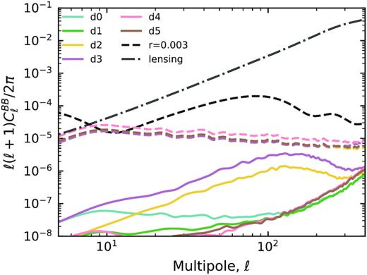
Residual B-mode power spectra for the different pysm Galactic dust models in the 150 GHz frequency band scanned using the BR3 HWP configuration. The solid lines use a value of the HWP angle offset that is tailored to each dust model (the median of the distributions shown in Fig. 6). The dashed coloured lines use the median of the rotation angle offsets calculated for the case of an SED given by the combination of CMB and dust.
Similar to the previous section, we also explore the case in which a single angle calculated for the SED of the combination of CMB and dust is used to correct for the HWP-induced rotation angle. These residuals are given by the dashed lines in Fig. 9. We again see that this choice of correction angle would produce significant residual and we see that this result is insensitive to the choice of dust model.
4.4 Scanning with a non-ideal beam
The simulation framework presented in this paper enables studies of the complicated interplay between non-ideal HWPs and non-ideal beams. For this purpose, we can use physical optics (PO) simulations that include extended beam sidelobes with non-negligible cross-polar response; features that could be present in an optical configuration shown in Fig. 1. The azimuthally averaged beam profiles for the Stokes Q and U beams of a representative beam used in this analysis are shown in Fig. 3. We study two cases, one where we apodize the beam maps at 3° away from the beam centre (no far-sidelobes) and one where we extend our beam maps out to 30° (with far-sidelobes). In order to focus on effects from the interplay between the beam and the HWP, we calculate difference maps by subtracting a map generated using the same beam model but with an ideal HWP.
Fig. 10 shows the resultant B-mode residuals; the input sky is the d1 dust model, the amplitude of the curves should be compared to the solid d1 curve in Fig. 9. The effect of the more complex beam model is two-fold. The increased solid angle of the beam, i.e. the sidelobe, brings in E-mode dust signal from behind the Galactic mask. Given that we use a correction for the HWP rotation angle offset φ that has been calculated for unmasked pixels, the correction that we apply is not quite appropriate for this extra signal. The result is E → B leakage close to the edges of the mask. The second, more significant, effect is due to the cross-polar beam. This is especially obvious in the right-hand panel of Fig. 10 that was made with the beam model that extends out to 30° and includes a relatively large cross-polar component. The impact of the cross-polar beam can be understood as an ℓ-dependent polarization rotation that, given the shape of the cross-polar component in Fig. 3, is larger at lower ℓ. One might wonder why the resulting E → B leakage is not cancelled in our set-up when we subtract the ideal-HWP maps that were created using the same cross-polar beam. The reason is that the dominant HWP non-ideality couples directly to the cross-polar beam component: the two effects are not additive but multiplicative. This can be seen in the third line of equation (16): the dominant 4να term of the data model contains a term proportional to |$\smash{\widetilde{U}^{(0)}_{\mathrm{b}}C_{P^* P}}$|, i.e. the product of the cross-polar beam and the P*P component of the HWP Mueller matrix in equation (A36). Roughly speaking, the difference maps used to create the spectra in Fig. 10 are thus proportional to the cross-polar beam times |$(1 - C_{P^* P})$|, the deviation from the ideal HWP Mueller element. The outcome is E → B leakage from the HWP non-ideality that is modulated by the cross-polar beam, resulting in the leaking of a redder version of the original E-mode dust spectrum to the B-mode spectrum, as can be observed in the right-hand panel of Fig. 10.
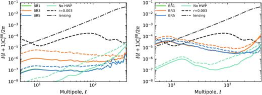
Left: Residual B-mode power spectra at 95 GHz (solid lines) and 150 GHz (dashed lines) derived from the band-averaged difference maps obtained by observing the pysm d1 dust model using all of the HWP configurations presented in Table 1 for scans with a PO beam truncated at 3°. Right: The same, but now observing the sky with a PO beam that extends to 30° and therefore includes a higher contribution from sidelobes (see Fig. 3). Note that the BR1 curves are almost completely hidden behind the BR5 curves.
4.5 Polarization sensitivity
Given the results that we have discussed so far, there does not seem to be much difference between the BR1 and BR5 performance. Both outperform the BR3 HWP configuration in all the tests we presented and in Fig. 10 the BR1 and BR5 curves overlap almost perfectly. However, the calibration process that we described in Section 4.1 masks the fact that the BR5 configuration has much greater polarization modulation efficiency than the BR1 configuration. For example, in the case when we scan the CMB with a Gaussian beam (see Section 4.2, Fig. 7), we find that the calibration coefficients based on the E-mode power spectrum are 1.44, 1.10, 1.09, and 1.00 for the BR1, BR3, BR5, and no HWP configurations, respectively. In comparison, the calibration procedure that uses the temperature power spectrum gives 1.04, 1.05, 1.08, and 1.00, for the BR1, BR3, BR5, and no-HWP configurations, respectively. This shows that even though the BR5 configuration has lower optical efficiency because of the larger number of optical elements, and therefore a greater number of both loss and reflection mechanisms, its polarization modulation efficiency, and therefore sensitivity, is approximately 15 per cent higher than that of the BR1 configuration when integrated over the 95-GHz band.
5 CONCLUSIONS
We formulated an extension of the harmonic beam convolution algorithm originally described by Wandelt & Górski (2001) that adds the capability of simulating systematics due to non-ideal HWPs. The generalized algorithm allows for numerically efficient generation of simulated time-domain data that include spurious signal from non-ideal HWPs and asymmetric and/or non-trivially polarized beams. Such time-domain simulations are a crucial part of ‘end-to-end’ analysis pipeline validation efforts for CMB experiments. As multiple current and upcoming CMB instruments employ HWPs, it is timely to include the associated non-idealities in our simulations. The new simulator also allows us to investigate the importance of HWP-related systematics, some of which we have investigated in this paper. The extended algorithm is implemented as part of the publicly available beamconv code, which has also been used to derive the results in this paper.
For our investigation into HWP systematics, we included three different HWP configurations: a one-, three-, and five-layer model. With this selection, we simulated data for a representative CMB B-mode satellite experiment that employs a spinning HWP as polarization modulator. Particular attention was paid to the frequency dependence of the system. Our simulated experiment employs dichroic detectors and is thus especially sensitive to frequency-dependent HWP systematics given the wide frequency band of the detectors.
We find that the choice of HWP configuration significantly impacts the B-mode reconstruction fidelity. In particular, the three-layer HWP that we study comes with a significant frequency-dependent rotation angle offset, which, if not corrected for, acts as a polarization angle offset that leaks E-mode to B-mode polarization by an amount that would be problematic for an experiment aiming to constrain the tensor-to-scalar ratio r to a level of r < 0.003. Correcting for the rotation offset requires a correcting HWP angle offset φ that is dependent on the SED of the observed signal; we demonstrate that φ varies significantly between the CMB signal and the Galactic dust signal. This introduces a challenge for the standard CMB data analysis paradigm, which aims to compress an experiment’s TOD into unbiased sky maps before component separation and cosmological analysis is performed. During this map-making procedure one typically has no knowledge of the relative contribution of each sky component to the TOD. As a result, the map-making procedure can only be given a single φ angle, based on some combination of the optimal φ of each of the sky components, which will necessary lead to biased maps. Parametric algorithms for component separation, starting from a prior on the SEDs of the various sky components, could use φ as a parameter per sky component and forward propagate the polarization rotation. Such algorithms might attempt to divine the φ angles from the observed amount of EB signal in the non-component separated maps, as no significant EB power has until now been observed for either dust or the CMB (Planck Collaboration XI 2020b).
In light of HWP rotation angle offsets that vary between sky components, we investigate how well one would need to know the SED of polarized Galactic dust when modelling the angle offset of this component. We find that the current understanding of the dust SED will likely suffice for this procedure. We determine offset angles for a range of different dust models and find that the resulting angles vary by an insignificant amount. Spatial variations in the dust SED also seem to be of relatively minor importance.
Finally, we leverage the potential of the new code by simulating data using non-ideal HWPs and non-ideal instrumental beams. We point out that there exist an interplay between the cross-polar component of the beam and certain HWP non-idealities. We find significant B-mode residual for all three HWP configurations when this interplay is not modelled correctly. We can conclude that a thorough understanding of the instrumental beam will be necessary for future experiments attempting to model or correct for HWP non-idealities.
ACKNOWLEDGEMENTS
We are grateful to Aurelien Fraisse, Brandon Hensley, Jo Dunkley, Tomotake Matsumura, and Hans Kristian Eriksen for helpful comments. Computations have been performed at the Owl Cluster funded by the University of Oslo and the Research Council of Norway through grant 250672. MB acknowledges the financial support from the COSMOS network (www.cosmosnet.it) through the ASI (Italian Space Agency) Grants 2016-24-H.0 and 2016-24-H.1-2018. JEG acknowledges support from the Swedish National Space Agency (SNSA/Rymdstyrelsen) and the Swedish Research Council (Reg. no. 2019-03959). Some of the results in this paper have been derived using the healpix (Górski et al. 2005) package.
DATA AVAILABILITY STATEMENT
The data underlying this article will be shared on reasonable request to the corresponding author.
Footnotes
The amplitude of incoming linear polarization |$\sqrt{Q^2 + U^2}$| will be changed based on the QQ, QU, UQ, UU submatrix. The change in amplitude will be bounded by the singular values of this matrix. Note that the amplitude change will generally be different per pixel and frequency. Furthermore, the input I and V signal will also alter the linear polarization amplitude due to leakage caused by the QI, UI, QV, and UV terms.
REFERENCES
APPENDIX A: EXPANDING ON THE MATHEMATICAL FRAMEWORK
The aim of this appendix is to give a more exhaustive explanation of the mathematical framework used in Section 2. In particular, we will derive the harmonic-domain version of the data model of equation (11) and derive the harmonic coefficients in equations (15)–(17).
