


ABSTRACT
We examine the stacked thermal Sunyaev–Zel’dovich (SZ) signals for a sample of galaxy group and cluster candidates from the 24 deg2 infrared Spitzer-HETDEX Exploratory Large Area (SHELA) survey. We identify the objects in combination with optical data using the redMaPPer algorithm, and divide them into three richness bins (λ in 10–20, 20–30, and 30–76 with average photometric redshifts of 0.80, 0.73, and 0.70, respectively). All richness bins show evidence for dust emission, which we fit using stacked profiles from Herschel Stripe 82 data. We fit for synchrotron emission using stacked profiles created by binning source fluxes from NRAO VLA Sky Survey data. We can confidently detect the SZ decrement only in the highest richness bin, finding MSZ,500 = |$8.7^{+1.7}_{-1.3} \times 10^{13}\, \mathrm{ M}_\odot$|. Neglecting the correction for dust and synchrotron depresses the inferred mass by 26 per cent, indicating a partial fill-in of the SZ decrement from dust and synchrotron emission. We compare our corrected SZ masses to two redMaPPer mass–richness scaling relations and find that the SZ mass is lower than predicted by the richness. For the lower richness bins, mass bias factors as low as 1 − b = 0.6 are not enough to bring the mass limits into agreement. We discuss possible explanations for this discrepancy. The SHELA richnesses may differ from previous richness measurements due to the inclusion of infrared data in redMaPPer. To connect the SZ signal to the mass, we use a universal gas pressure profile that is calibrated to massive clusters at low redshift. It may not be applicable to our lower mass, higher redshift sample.
1 INTRODUCTION
Clusters of galaxies are the largest gravitationally bound structures in the Universe. They are powerful cosmological probes because they sample the maxima of the primordial density field, and allow us to gain insight into large-scale structure, galaxy evolution, dark matter dynamics, and cosmological parameters (Birkinshaw 1999; Carlstrom, Holder & Reese 2002; Voit 2005). The thermal Sunyaev–Zel’dovich (SZ) spectral distortion of the cosmic microwave background (CMB; Sunyaev & Zeldovich 1972) can be used as an indirect measurement of one of the most important observables – total galaxy cluster mass – and can identify clusters to high redshift (Bleem et al. 2015; Planck Collaboration XXVII 2016c; Burenin et al. 2018; Hilton et al. 2018; Khullar et al. 2019). The SZ effect occurs when CMB photons scatter from the hot electron gas in the intracluster medium. Only a small fraction of the photons interact: a 1014 M⊙ cluster has a 1.3-arcmin-aperture-averaged optical depth of τ ∼ 2 × 10⁻³ (Battaglia 2016). The photons gain energy through inverse Compton scattering, which alters the observed CMB spectrum and results in a characteristic spectral dependence for the SZ effect: a flux decrement for frequencies below 217 GHz and a flux increment for higher frequencies (Sunyaev & Zeldovich 1972). The magnitude of the effect is proportional to the Comptonization parameter (the integrated electron pressure), and the pressure is proportional to the depth of the gravitational potential well. Therefore, the amplitude of the SZ signal depends closely, but not linearly, on the mass of the cluster. Using the SZ effect for cosmology requires an understanding of this relationship between the halo mass and the SZ observable, which is often expressed as the Comptonization parameter integrated over the cluster’s solid angle. Since the SZ effect is a distortion of the CMB’s spectrum, the signal does not decrease with distance the way that the cluster emission does, so the SZ effect is an efficient way to find high-redshift clusters, limited only by the mass of the cluster and the sensitivity of the telescope.
For high-mass clusters, |$M \gtrsim 10^{15}\, \mathrm{ M}_\odot$|, current SZ searches can already find haloes efficiently at all redshifts, but for lower mass groups, M ≲ 1014 M⊙, it becomes more difficult. These lower mass haloes are interesting because their smaller potential wells have a harder time holding on to their gas, and are laboratories for star formation and active galactive nuclei (AGN) feedback (Balogh et al. 2011; Laganá et al. 2013; Liu et al. 2015). Although studies of low-mass haloes using the SZ effect will become more common as CMB telescopes become more sensitive, for now we depend on stacking, or averaging, multiple clusters that have been detected by other means. Spatially coherent stacking allows the use of the SZ effect to extend to lower masses, as it averages out contributions from the CMB, atmosphere, and detector noise (Hand et al. 2011; Planck Collaboration XII 2011; Sehgal et al. 2013; Saro et al. 2017).
At low redshift, optical surveys can identify clusters efficiently with multiband overdensity finders, e.g. MaxBCG (Koester et al. 2007), redMaPPer (Rykoff et al. 2014), and CAMIRA (Oguri 2014). At higher redshift, the infrared (IR) becomes an efficient avenue of detection, e.g. MaDCoWS (Stanford et al. 2014; Gonzalez et al. 2019), ISCS (Eisenhardt et al. 2008), IDCS (Stanford et al. 2012), RCS (Gladders & Yee 2000), and several Spitzer catalogues (Papovich 2008; Papovich et al. 2010).
The SZ signals of low-richness, optically selected objects are smaller than expected from mass–richness relationships, which are usually calibrated with high-richness clusters (Planck Collaboration XII 2011; Draper et al. 2012; Sehgal et al. 2013; Saro et al. 2017). Several possible explanations for this discrepancy are radio or infrared point source contamination of the SZ signal, line-of-sight projections contaminating richness measurements, cluster miscentring, variable gas mass fractions in optically selected clusters, or more fundamentally, a lower amplitude for the mass–richness relation. Additionally, cluster gas profile models (like Arnaud et al. 2010), which are a means to translate from the mass to the SZ signal, are calibrated with low-redshift, moderate- to high-mass objects, and may not be applicable to high-redshift, low-mass objects. Solving this richness–SZ signal discrepancy is vital so that scaling relations for clusters, and therefore cluster physics, are understood over a wide mass range, allowing clusters to be used to their full cosmological potential.
In this work, we look for the SZ signal in data from the Atacama Cosmology Telescope (ACT), using cluster candidates selected by the redMaPPer algorithm from catalogues of multiwavelength imaging, including Spitzer data from the Spitzer-HETDEX Exploratory Large Area (SHELA) survey. The resulting sample is higher in redshift and lower in mass than many other samples. Using Herschel and NRAO VLA Sky Survey (NVSS) data, we correct the stacked SZ decrement for contamination from dust and synchrotron emission, while simultaneously fitting for a halo mass based on the stacked SZ signal. We characterize the uncertainty with a Markov chain Monte Carlo (MCMC) method. We also compare the sample’s SZ masses to optical mass–richness relationships.
We adopt a flat Lambda cold dark matter (ΛCDM) cosmology with parameters from Planck Collaboration XIII (2016a): H0 = 67.3 km s−1 Mpc−1 and Ωm = 0.315. The mass M500 is measured out to R500, which is the radius enclosing 500 times the critical density at a given redshift.
This paper is organized as follows: In Section 2, we introduce the cluster sample, the ACT and ACTPol data, the Herschel data, and the NVSS data used in this analysis. In Section 3, we describe the methods we used to analyse the data. These include the filtering and stacking procedures, calculation of the covariance matrices, and a discussion of the noise and signals that contribute to the stacked profiles. We describe our resulting multifrequency stacked profiles and discuss our methods for removing dust and synchrotron contamination. We describe our fitting procedure, including the SZ and pressure profile we use to translate our SZ signal into a cluster mass. In Section 4, we present the results of our analysis and discuss how our SZ masses scale with richness. In Section 5, we conclude with a discussion of the analysis and results.
2 DATA
2.1 Cluster sample
The sample contains IR- and optically selected redMaPPer cluster candidates from the SHELA (Papovich et al. 2016). SHELA is a 24-deg2 IRAC 3.6-and 4.5-µm survey in a low-IR background region of Stripe 82 (York et al. 2000), centred at a right ascension of 1h22m00s on the celestial equator, and extending ±6|${_{.}^{\circ}}$|5 in right ascension and ±1|${_{.}^{\circ}}$|25 in declination. The SHELA survey region also includes Dark Energy Camera (DECam) ugriz imaging. Multiwavelength coverage in the same field includes Sloan Digital Sky Survey (SDSS) and Hobby-Eberly Telescope Dark Energy Experiment (HETDEX) in the optical, NOAO Extremely Wide-Field Infrared Imager in K band, Herschel in the sub-mm, and ACT in the microwave.
For this study, we use a galaxy catalogue based on DECam and SHELA imaging (Wold et al. 2019). We process the galaxy catalogue with the redMaPPer algorithm (Rykoff et al. 2014), resulting in a catalogue of 1082 groups and clusters with a richness λ ≥ 10. Richness is a measure of how many galaxies belong to a cluster. In redMaPPer, it is defined as the sum of the membership probabilities for the galaxies within a cluster.
We use clusters with richnesses λ ≥ 10, and break these into three richness bins: 10 ≤ λ < 20, 20 ≤ λ < 30, and λ ≥ 30. There are 840, 172, and 70 clusters in the lowest to highest richness bins, respectively. Two rich clusters from the SHELA sample have already been detected in the ACT SZ cluster sample in this area of the sky. The ACT-detected clusters are ACT-CL J0058.0+0030 with a signal-to-noise ratio (S/N) of 5.0 and ACT-CL J0059.1−0049 with an S/N of 8.4 (Hasselfield et al. 2013). None of the remaining objects are detected individually in SZ by ACT, so their individual masses must be roughly |$\le \, 10^{14}$| M⊙, ACT’s approximate mass limit.
In the relevant redshift range, z ∼ 0.7–0.8, the 90 per cent completeness limit for M500 in ACT is 4–5 × 10¹⁴ M⊙ (Hilton et al. 2018). Properties of each richness bin are summarized in Table 1.
Properties of the SHELA cluster candidate richness bins.
| λ range | 10–20 | 20–30 | 30–76 |
| Average λ | 14 | 24 | 39 |
| Nclusters | 840 | 172 | 70 |
| z range | 0.50–1.60 | 0.50–1.35 | 0.52–1.18 |
| Average z | 0.80 | 0.73 | 0.70 |
| λ range | 10–20 | 20–30 | 30–76 |
| Average λ | 14 | 24 | 39 |
| Nclusters | 840 | 172 | 70 |
| z range | 0.50–1.60 | 0.50–1.35 | 0.52–1.18 |
| Average z | 0.80 | 0.73 | 0.70 |
2.2 ACT millimeter-wave data
We use ACT data to measure the SZ decrement and null signals. ACT is a 6-m millimeter-wave telescope at an altitude of 5200 m on Cerro Toco in the Chilean Atacama Desert (Swetz et al. 2011). It surveys the CMB with high resolution and sensitivity. The first generation of ACT observations dates from 2007 to 2010; there were three detector arrays operating at frequencies of 148, 220, and 277 GHz. These bands were chosen to study the SZ and capture the SZ decrement, null, and increment. ACT surveyed two regions on the sky, the ‘southern’ and ‘equatorial’ surveys. The southern survey covered 455 deg2 and is centred on declination −53.5° (Marriage et al. 2011). The equatorial survey overlaps with 270 deg2 of Stripe 82 and the entire SHELA survey, covering 504 deg2 and spanning from 20h16m00s to 3h52m24s in right ascension and −2°07′ to 2°18′ in declination (Hasselfield et al. 2013). The second generation of the experiment, ACTPol, was deployed in 2013 (Thornton et al. 2016). It has receivers at 90 and 148 GHz, polarization capability, and triple the sensitivity of ACT. ACTPol has made observations in four deep field patches and one wider field (Naess et al. 2014; Hilton et al. 2018). The wider ‘D56’ region overlaps with SHELA, covers 548 deg2, is centred on the celestial equator, and expands the area covered by ACT.1 In this work, we measure the SZ decrement using coadded, point source subtracted, ACT temperature maps at 148 GHz from all observing seasons that overlap with the SHELA survey region: seasons 3–4 (2009 and 2010) of ACT and season 2 (2014) of ACTPol. The ACT maps have 0.495 arcmin pixels, while the ACTPol maps have 0.5 arcmin pixels. We use ACT maps that have been repixelized into the ACTPol pixelization to make coadded maps of all available data. From seasons 3–4 of ACT, we use data at 220 GHz, a frequency near the SZ null, to constrain contamination from thermal dust and synchrotron emission. These maps are also repixelized into the ACTPol pixelization. At full width at half-maximum (FWHM), the beam sizes are 1.4 arcmin at 148 GHz, and 1.0 arcmin at 220 GHz.
2.3 Herschel submillimeter data
To measure dust emission from cluster member galaxies, we use far-IR data from the Herschel Stripe 82 (HerS) survey, which consists of maps at 250, 350, and 500 µm (or 1200, 857, 600 GHz) observed with Herschel/SPIRE (Viero et al. 2014). The survey covers 79 deg2, spanning 13° to 37° in right ascension and −2° to +2° in declination. The SPIRE beams are 18.2, 25.2, and 36.3 arcsec at 1200, 857, 600 GHz, respectively. In addition to the maps, in this work we use the band-merged source catalogue from the HerS team, which contains compact source flux densities and uncertainties in each band. The HerS team assumed sources are point-like and they identified them using the IDL software package starfinder (Diolaiti et al. 2000). They produced the band-merged catalogue using the De-blended SPIRE Photometry (desphot) algorithm, which uses source positions from the 1200 GHz band as a prior for the other frequencies (Roseboom et al. 2010).
2.4 NVSS radio data
To measure synchrotron emission from cluster member galaxies, we use 1.4-GHz data from the NRAO VLA Sky Survey (NVSS), which covers the sky North of declination −40° (Condon et al. 1998). We use flux densities and uncertainties from the source catalogue, which contains around 106 sources brighter than approximately 2.5 mJy. From the lowest to highest richness bin, respectively, there are 5428, 1127, and 485 total sources within 9 arcmin-radius apertures centred on the clusters.
3 METHODS
Our overall strategy in this analysis is to build up a model for the stacked emission in the ACT bands at the location of the clusters, allowing for SZ, dust, and synchrotron components. We estimate the data’s covariance due to CMB and noise fluctuations, and then use Markov Chain Monte Carlo chains to estimate the parameters of our emission model.
3.1 SZ Profiles
3.2 Map filtering and stacking
Before stacking, we filter the maps using a high-pass filter designed to lessen the impact of large-scale CMB fluctuations while minimally altering the small-scale cluster signal. To avoid bias, we design a filter independent of any assumed cluster shape. Our filter is a Fourier-space high-pass filter that we define in terms of its low-pass complement. The low-pass complement in real space is an apodized top-hat. It is unity inside 3-arcmin radius and tapers to zero outside of 5 arcmin with a cosine transition. Thus our high-pass filter removes the large-scale features in the map, and barely touches small harmonic scales. Our filter is not matched to any specific cluster profile, and leaves much of the small-scale detector white noise in the data. A less aggressive filter that tapers to zero between 9 and 11 arcmin produces profiles consistent with those shown in Fig. 2. When compared, all maps, simulations, and model cluster profiles are subjected to this same filter.
Our results are robust to changes in this filter. As a test, we modified the filter to introduce beam smoothing. The filter is the same high-pass filter used for the analysis, but convolved with the beam at 148 GHz to reduce pixel-scale white noise. This resulted in smoother, shallower profiles, but the mass estimates were similar to those reported in this analysis, with higher uncertainty as there was more bin to bin correlation.
Most of the cluster candidates were not individually detected in SZ by ACT. To increase the signal-to-noise we stack, or average, observations of the clusters together into 30 annular bins, centred on the redMaPPer cluster positions, out to a radial separation of 9 arcmin, which is chosen to be past the filtering scale. CMB and white noise fluctuations have zero mean therefore stacking observations partially averages out these noise fluctuations. Measurements for a given pixel are placed in the radial bin in which the centre of that pixel falls.
The ACT beams (b148, b220) include the smoothing effects of the pixel window and the telescope pointing jitter. There is little SZ signal at 220 GHz, so we can use this profile to estimate the contributions from dust and synchrotron emission in the ACT bands. The models we use to estimate Pdust and Psynch are discussed in Sections 3.5 and 3.6, respectively.
3.3 Covariance matrices
In the ACT frequencies, 148 and 220 GHz, the error in each annular bin of the stacked profile reflects the covariance introduced by CMB fluctuations, detector noise, and atmosphere. The covariance matrix is calculated by carrying out the same filtering and stacking procedure on 1600 simulations that model coadded ACT and ACTPol maps. As a first step, we make a coadded data map by repixelizing the ACT maps into the new ACTPol pixelization, and sum up all the different seasons and arrays. We use the power spectra of that coadded data to generate CMB plus noise simulations. These account for cross-correlations between 148 and 220 GHz present in the data (chiefly due to the CMB, but also correlated atmosphere). The mock maps are then filtered the same way as the data prior to stacking. After filtering, and for each richness bin, we stack on each of the 1600 simulations at the actual locations of the SHELA clusters. Using the actual locations helps to capture the correct correlations from the random realizations of CMB and noise. We use the stacked profiles to compute the covariance between the annular bins. The covariance is largest in the small angle bins where there are few measurements to average down the noise. We compute the correlation matrix from the covariance matrix (which normalizes the diagonal) and show it in Fig. 1 for each richness bin at 148 GHz. Note the correlations between the annular bins, which later go into our assessments of goodness of fit.
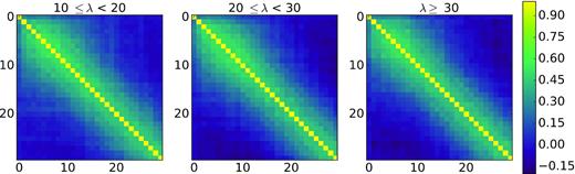
Correlation matrices for the stacked pressure profiles at 148 GHz for the three richness bins, 10 ≤ λ < 20 (left), 20 ≤ λ < 30 (middle), and λ ≥ 30 (right). They are obtained by stacking on 1600 simulations of ACT that contain correlations introduced by CMB fluctuations, detector noise, and atmospheric noise, and account for the different observing seasons of ACT used in this analysis. Adjacent bins are correlated at ∼0.5. The axes label the radial bin numbers, which extend to 9 arcmin.
Errors on the dust SED, dust profiles, and synchrotron profiles also figure into our final uncertainties. The HerS catalogue includes 1σ uncertainties for the flux density of each source, which we use by averaging in quadrature for the SED fitting process. The error bars on the stacked Herschel profiles come from stacking on the survey’s noise maps. The covariances of the stacked NVSS profiles come from binning the variance of each source flux and smoothing with the appropriate ACT beam and filter to account for the bin-to-bin correlation.
3.4 Multifrequency profiles
The stacked profiles for the different richness bins are shown in Fig. 2. The profiles show the cluster-centred emission for NVSS sources at 1.4 GHz, ACT at 148 and 220 GHz, and the three HerS bands (600–1200 GHz).2 Here, as an example, we plot the synchrotron profile and error bars smoothed with the 148-GHz beam. The ACT profiles at 148 GHz do not show an SZ decrement at high significance, but any decrement is subject to being filled in by the dust emission and synchrotron emission, which are two mechanisms we want to constrain. We expect the stacks at 220 GHz to contain little SZ signal, but they do show clear cluster-centred emission. We use this 220-GHz emission profile to constrain the dust and synchrotron components. We also show profiles from the HerS maps at 500, 350, and 250 µm that we use to fit for dust. We have fit and removed offsets in the profiles at radii larger than 5 arcmin. The error bars on the stacked HerS profiles result from stacking on the noise maps provided with the HerS data.
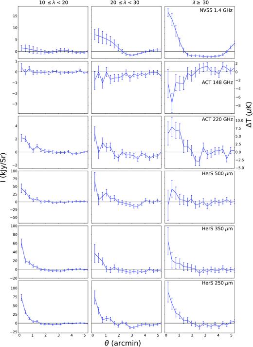
Stacked profiles of the three richness bins for all 6 bands used in this analysis: NVSS at 1.4 GHz, ACT at 148 GHz and 220 GHz, and HerS at 500, 350, and 250 µm. The main contributions to the profile at 148 GHz are the SZ signal and dust and synchrotron emission. ACT 220 GHz is near the SZ null, and shows emission that also contaminates the signal at 148 GHz. The Herschel bands (500, 350, 250 |$\rm \mu m$|) trace thermal dust emission in the clusters, and the profiles are the result of stacking on each frequency map and subtracting DC offsets from radii >5 arcmin. The NVSS stacks trace synchrotron emission, and the profiles result from binning NVSS sources based on their angular separation from the cluster centres and smoothing with the ACT 148-GHz beam. The NVSS stacks sometimes go negative due to the hi-pass filtering, and the bins are highly covariant due to the beam smoothing. The error bars are the diagonal of the covariances described in the text. All profiles are filtered with the high-pass filter. We plot our stacked profiles out to a radius of 5 arcmin to highlight the cluster-centred emission.
The ACT 220 GHz, NVSS, and Herschel stacks demonstrate that there is a signal from dust and synchrotron emission within a few arcmin radius of the cluster centres: compared to the null hypothesis of zero emission, the probabilities to exceed χ2 for the ACT 220-GHz profiles and the nine Herschel profiles shown in Fig. 2 are each <0.05, so we conclude that cluster-centred emission is present. For the NVSS profiles, we calculate the probability to exceed χ2 before they are smoothed with the ACT 148 beam, and find values that are also <0.05. (Fig. 2 shows them after smoothing.) The probability to exceed χ2 for the ACT 148 profiles are 0.69, 0.35, and 0.03, respectively, for the lowest to highest richness bins.
To test the robustness of the noise model, and that our signals are not merely a feature caused by the stacking procedure, we stack on random positions in the ACT maps, and find no signal on average. Fig. 3 shows the results from stacking on random positions in the 148-GHz map, with each null stack accounting for the number of clusters in the different richness bins. We use the full covariance to compute χ2. The probabilities to exceed χ2 for the random position stacks are 0.47, 0.45, and 0.35, respectively, for the lowest-to-highest richness bin, consistent with no emission in the null stacks. When stacking on the same random positions in the 220-GHz map, the probabilities to exceed χ2 are 0.12, 0.35, 0.70, from the lowest-to-highest richness bin.
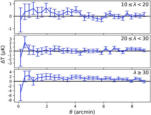
Stacking null test at 148 GHz. We generate random positions for the number of clusters in each richness bin and stack the ACT map in those locations to test that there is no signal in places unassociated with clusters. Although the bottom bin has an offset, it has the smallest number of objects so is most subject to large-scale fluctuations. Assessed by the χ2, none of these random samples have a significant signal, as expected. The evaluation of χ2 accounts for the bin-to-bin correlations (Fig. 1).
3.5 Dusty source contamination
Emission from dusty sources and radio sources contaminates the SZ signal in clusters (Aghanim, Hansen & Lagache 2005). As seen in Fig. 2, when stacking at 220 GHz (the SZ null) and higher frequencies, there is an excess signal, which we partially attribute to dust emission from cluster member galaxies. This positive emission will also be present at 148 GHz, where it fills in the SZ decrement, causing the sample to appear to have less than its true mass. To correct for this, we fit for a dust component at 148 and 220 GHz.
From the HerS survey source catalogue (Viero et al. 2014), we use the summed source flux within an 11-arcmin-radius aperture around our clusters. The Herschel source fluxes let us infer S(ν), and scale the Herschel map stacks down to the ACT frequencies. After scaling the Herschel stacks to the ACT bands, we deconvolve the Herschel beams and reconvolve with the appropriate ACT beams. We fix the emissivity spectral index βdust to 1.5, ν0 to 100 GHz, and the redshift to the average redshift for each of the richness bins. Magnelli et al. (2014) find that setting βdust to 1.5 is a good estimate when fitting spectra without enough information to constrain it, and note that it may cause Tdust to be slightly overestimated. Furthermore, when fitting for a stacked SZ plus greybody spectrum for Planck galaxy clusters, Erler et al. (2018) found that the choice of βdust had little influence on the measured SZ signal, and use βdust = 1.5 to obtain their main results. We ran our pipeline on the data from the highest richness bin using βdust = 1.4 and 1.6 to see how βdust affects our results. We found that varying βdust did not significantly affect the mass estimates; the differences were less than 0.1σ. We report results with SED fitting to HerS sources with an 11 arcmin aperture in Table 2 to take into account all sources near the clusters, but the results are not sensitive to the precise aperture used.
Best-fitting parameters for fitting an SZ profile in two ways: correcting for dust and synchrotron emission, and neglecting the dust and synchrotron correction.
| 10 ≤ λ < 20 | 20 ≤ λ < 30 | λ ≥ 30 | ||||
|---|---|---|---|---|---|---|
| Corr. | No corr. | Corr. | No corr. | Corr. | No corr. | |
| M500 (1013 M⊙) | < 1.9 | < 1.1 | < 4.4 | < 3.1 | |$8.7^{+1.7}_{-1.3}$| | |$6.4^{+1.3}_{-1.3}$| |
| |$p_0^{148} \ (\rm Jy\,sr^{ -1})$| | −20 ± 40 | |$-10^{+45}_{-50}$| | |$-10^{+75}_{-80}$| | |$-10^{+75}_{-80}$| | −100 ± 130 | |$-90^{+130}_{-150}$| |
| |$p_0^{220} \ (\rm Jy\,sr^{ -1})$| | 50 ± 70 | – | |$-140^{+130}_{-140}$| | – | 7 ± 220 | – |
| |$T_{\rm dust} \ (\rm K)$| | |$29.1^{+0.1}_{-0.1}$| | – | |$28.0^{+0.1}_{-0.1}$| | – | |$27.0^{+0.2}_{-0.2}$| | – |
| |$A^{220}_{\rm dust} \ (\rm mJy)$| | 0.264 ± 0.001 | – | 0.268 ± 0.002 | – | 0.350 ± 0.003 | – |
| |$A^{220}_{\rm synch} \ (\rm mJy)$| | < 0.5 | – | < 0.5 | – | <1.5 | – |
Note.Resulting fit parameters for the three richness bins. The first column for each richness bin shows results from fitting for dust and synchrotron contamination simultaneously with the SZ profile, fixed at the average redshift for each sample, assuming no mass bias. The second column lists the results if we neglect the dust and synchrotron correction and fit an SZ profile directly to the raw, stacked 148-GHz profile.
3.6 Radio source contamination
The 1.4 GHz synchrotron profile |$P^{1.4}_{\rm synch}$| comes from summing the flux density of sources from the NVSS catalogue into the bins used for all the stacking in this paper, and dividing the resulting profile by the solid angle in each bin. The profile is then normalized to unit integral over solid angle so that |$A^{220}_{\rm synch}$| has dimensions of flux density. When being compared to the stacks at 148 and 220 GHz, the model synchrotron profile is filtered with the same filter used in the analysis, and smoothed by the beam for the appropriate ACT frequency. Our data cannot constrain the spectral index, αsynch, so we apply a prior to our MCMC fitting procedure, which is based on ACT and Planck measurements. When using ACT data and fitting AGN for synchrotron, SZ, and IR emission, Gralla et al. (2014) measured αsynch = −0.55 ± 0.03. For a sample of DSFG’s and AGN, Marsden et al. (2014) find a spectral index between 148 and 218 GHZ of |$\alpha ^{148-218}_{\rm synch} = -0.55 \pm 0.60$|. Marriage et al. (2011) find |$\alpha ^{20-148}_{\rm synch} = -0.39 \pm 0.04$| and |$\alpha ^{5-148}_{\rm synch} = -0.20 \pm 0.03$|. There have been several Planck studies measuring the spectral index of radio sources. For several classes of radio sources, αsynch was measured to range between |$\sim \, -$|0.37 and −0.78 (Planck Collaboration XLV 2016d), and when scaling from 30 GHz, the spectral indices for extragalactic sources were measured to be −0.39 and −0.37 when scaling to 143 and 217 GHz, respectively (Planck Collaboration XII 2011). Given this information, we have placed a prior on αsynch that is a Gaussian distribution with a mean of −0.5. We fixed the prior standard deviation to 0.2, and then tested how adjusting the width of the distribution affects our SZ mass estimates. Adjusting the prior’s standard deviation to 0.1, 0.4, and 0.6 resulted in masses that were within 0.05σ of our original mass estimate, and did not affect the uncertainty in the estimate.
3.7 Multifrequency likelihood
To account for the corrections in the mass fitting, we simultaneously fit for SZ, dust, and synchrotron contributions to the stacked profiles. We use a Gaussian likelihood and the affine-invariant MCMC code emcee (Foreman-Mackey et al. 2013). The fit parameters are the average cluster mass M500, overall DC offsets for the stacked profiles at 148 and 220 GHz, |$p_0^{148}$| and |$p_0^{220}$|, an amplitude for the greybody SED Adust, a dust temperature Tdust, an amplitude for the synchrotron emission at 220 GHz |$A_{\rm synch}^{220}$|, and a spectral index for the synchrotron scaling αsynch. We fix the redshift dependence of the dust spectrum (equation 10) and SZ signal (equation 4, and calculations of R500 and ρc) to the average redshift for each sample, z = 0.80, 0.73, and 0.70, for the lowest-to-highest richness bins. We apply flat priors which enforce that M500, Adust, Tdust, and |$A_{\rm synch}^{220}$| are positive, and place wide, flat priors on offsets |$p_0^{148}$| and |$p_0^{220}$|. The prior for αsynch is a Gaussian centred on −0.5, with a standard deviation of 0.2, as discussed in Section 3.6.
For each step in the sampler, the sampled mass is used to calculate the SZ signal y(θ) (Section 3), which is convolved with the ACT beam and translated into a temperature profile, ΔT(θ). The sampled dust parameters, Adust and Tdust are used to calculate a dust SED and compared to the HerS flux densities, and determine how to scale the HerS profiles to 148 and 220 GHz. The shape of the synchrotron profile is used with the sampled values for |$A_{\rm synch}^{220}$| and αsynch to estimate the synchrotron contribution at 148 and 220 GHz.
The SZ signal does not scale linearly with mass, and choosing one mass value to compare with our stacked profiles may cause us to infer a value for M500 that is not characteristic of the clusters in the sample. To address this, we tested a second-fitting method that uses a weighted average of SZ profiles to compare with our stacked profile. We start with the richness distribution of the clusters in each bin, and use the mass–richness relation of Saro et al. (2015) to translate the richness distribution into a mass distribution. For each mass |$M_{500}^{\rm MCMC}$| that is sampled in the MCMC, we shift the mass probability density distribution to have a mean which is |$M_{500}^{\rm MCMC}$|, and scale the probabilities accordingly. Then we perform a weighted average of the SZ signal with a range of masses, where the weights are the probabilities from the new mass probability density distribution. The masses that we infer from this fitting method differ from the masses inferred in the main analysis by less than 0.1σ, but this correction may be more important with future, higher S/N data.
4 RESULTS
We use a MCMC method to fit the stacked profiles and infer M500. We then use richness information available from the IR and optical data to compare to other works.
4.1 Parameter constraints
Figs 4, 5, and 6 show the results from fitting the stacked profiles for SZ, dust, and synchrotron components. Fig. 4 shows the stacked profiles for the ACT bands in blue, as well as the most-likely models from the MCMC chains in green. The light green area encompasses 68 per cent of the models from the MCMC chains in each annular bin. We report the probability to exceed χ2 (PTE) for data minus model for the best-fitting model in each richness bin. These are computed jointly from the pair of stacks at 148 and 220 GHz and the full covariance matrix. We calculate the PTE’s of the models using 53 degrees of freedom, as there are 60 points in the two stacked profiles and 7 model parameters.
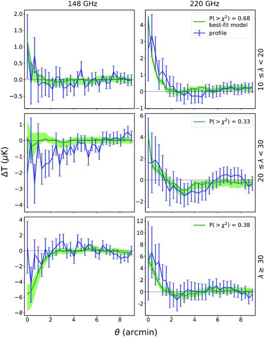
Results at 148 (left) and 220 GHz (right) from fitting for SZ and contaminating emission for the three richness bins. The blue line is the stacked profile. The green line is the most-likely profile for the combined SZ, dust, and synchrotron model, based on the MCMC chains. The lighter green band bounds the models in the chains between the 16th and 84th percentiles in each angular bin. The legends display the probability to exceed χ2 for the data minus the model, which takes into account the profiles and correlations at 148 and 220 GHz, as well as their cross-correlations. The PTE’s show that all are reasonable fits.
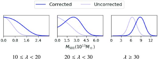
Mass distributions for the three richness bins when correcting for (dark blue) – or not correcting for (light blue) – dust and synchrotron contamination. We see no significant detection in the lowest richness bin. Accounting for contamination slightly increases the estimated masses for the higher richness bins.
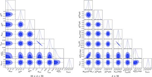
Parameter contours from MCMC chains for the lowest and highest richness bins. The grey dashed lines pass through the mean values from the probability distributions for each parameter. The dust amplitude and temperature are anti-correlated in all richness bins. The synchrotron emission is slightly better constrained for the richer sample, and somewhat correlated with the mass.
We show the mass distributions for the three richness bins in Fig. 5, correcting for (and neglecting to correct for) contaminating emission. For the lowest and highest richness cases, Fig. 6 shows all the parameter contours from the MCMC chains: M500, DC offsets in the 148 and 220 GHz stacks, a dust amplitude, a dust temperature, a synchrotron amplitude, and the scaling for the synchrotron spectrum. The synchrotron amplitude and SZ mass are correlated, and the dust temperature and amplitude are anticorrelated. The synchrotron amplitude runs into the lower prior of zero in the highest richness bin, and is consistent with zero for the lower richness bins.
In the lowest richness bin, the best-fitting model primarily shows dust emission and little evidence for an SZ signal. The mass distributions run into the prior limit of zero mass, whether correcting or not correcting for dust contamination.
In the middle richness bin, there is a mild preference for an SZ signal, indicated by the probability distribution for SZ mass peaking above zero in Fig. 5 when the dust is accounted for. In the model, the SZ decrement at 148 GHz is canceled by the source emission. The middle richness bin also shows a notable, broad decrement in the 148 GHz data. That decrement is too wide to fit successfully with an SZ profile, and we have tested that increasing the mass worsens χ2 compared to the best-fitting model. Large-scale CMB fluctuations and atmospheric noise have the spatial extent to cause of this behaviour, while the other astrophysical components tend to be too localized towards the cluster centre, and only the SZ is negative. The CMB and atmosphere are not part of the model, but are accounted for in the covariance matrix (Section 3). The PTE for the joint fit, P(> χ2) = 0.33, shows that this model is a reasonable fit to the data, despite the broad decrement. Considering the 148-GHz profile and its covariance on its own (without 220 GHz), the χ2 value of the data minus the model is χ2 = 31.96 for 30 bins. Based on our covariance matrices, χ2 values, and number of profiles we examine, we do not see strong evidence that this decrement is a wild outlier.
In the highest richness bin, we see a clear SZ detection. We make a significant mass detection whether or not we account for cluster-centred emission. Accounting for the contamination increases the mass.
The fit parameters are summarized in Table 2, which shows results from simultaneously fitting dust, synchrotron, and SZ components to the ACT data, as well as fitting an SZ profile directly to the data while neglecting to correct for dust and synchrotron emission. In the lower richness bins we report 95 per cent upper limits, as we do not make significant mass estimates. For the highest richness bin, we can use the maximum likelihood values for the fit parameters in Table 2 with SED equations (10) and (11) to calculate the ratio in the flux between 148 GHz and the NVSS/Herschel bands, finding that |$S^{\rm synch}_{148} = 0.097 \cdot S_{1.4}$|, |$S^{\rm dust}_{148} = 0.015 \cdot S_{500}$|, |$S^{\rm dust}_{148} = 0.007 \cdot S_{350}$|, and |$S^{\rm dust}_{148} = 0.005 \cdot S_{250}$|. (Note that the 1.4-GHz NVSS extrapolation may not be reliable because our 148–220 GHz synchrotron spectral index may not be valid down to 1.4 GHz.)
When accounting for dust and synchrotron emission, in the lowest richness bin we place a 95 per cent upper limit on the mass of |$M_{500} \le 1.2 \times 10^{13}\ \rm M_{\odot}$|. In the middle richness bin, |$M_{500} \le 4.4 \times 10^{13}\ \rm M_{\odot}$|. In the highest richness bin, we estimate an SZ mass of |$8.7^{+1.7}_{-1.3} \times 10^{13}\ \rm M_{\odot}$|. Neglecting to account for dust and synchrotron emission decreases the mass by 26 per cent in the highest richness bin.
As a robustness check, we use the random stacks from Fig. 3 to test what mass our pipeline measures when there is no signal. Fitting without a dust and synchrotron correction results in probabilities of measuring a mass that pushes up against the lower limit of the prior (zero mass). At 95 per cent confidence, the upper limit of the null mass distributions are |$1.9 \times 10^{13}$|, |$2.7 \times 10^{13}$|, and |$4.8 \times 10^{13} \rm M_{\odot}$|, for the lowest-to-highest richness bins. As another robustness check, we allow for a negative mass. We calculate PSZ using the absolute value of the sampled mass, and multiply the profile by −1 if the mass is below zero. In this case, we find that 50 per cent of the sampled masses are negative for the lowest richness bin, 65 per cent for the middle richness bin, and 26 per cent for the highest richness bin.
4.2 Impact of mass bias
The relation between SZ signal and cluster mass, Y–M, is often measured using X-ray derived cluster masses while assuming hydrostatic equilibrium (HE; Arnaud et al. 2010; Andersson et al. 2011), but there are several effects that cause these X-ray mass estimates to be biased low. For example, non-thermal pressure support from turbulence and random motions move the clusters away from perfect HE. Regardless of the cause, the bias between the true mass and the mass measured by the SZ effect can be quantified as 1 − b = MSZ/Mtrue. The value for 1 − b needs to be determined depending on the mass proxy and survey and could lie in a large range (Planck Collaboration XX 2014). In Planck Collaboration XX (2014), the bias is fixed at 1 − b = 0.8. On the other hand, Battaglia et al. (2016) measured the mass bias for high signal-to-noise clusters from the ACT equatorial survey, using weak-lensing data from the Canada–France–Hawaii telescope stripe 82 survey. They found that 1 − b = 0.98 ± 0.28 and 1 − b = 0.87 ± 0.27 when fitting the weak-lensing mass using models based on simulations and an NFW profile, respectively. Miyatake et al. (2019) present the amount of mass bias present in ACTPol clusters when comparing their SZ masses to weak lensing masses derived from Hyper-Suprime Cam data. They find |$1-b = 0.74^{+0.13}_{-0.12}$|. There have been several other measurements of 1 − b, with values ranging from 0.58 to 0.95 (von der Linden et al. 2014; Hoekstra et al. 2015; Planck Collaboration XXIV 2016b; Smith et al. 2016; Zubeldia & Challinor 2019). When comparing our measured MSZ to cluster mass scaling relations, we use the values: 1 − b = 1, 0.8, and 0.6. We choose these values to sample the range of values that have been measured, in order to demonstrate how different amounts of mass bias could affect our mass estimates.
4.3 Richness to mass scaling
We find that the SZ masses and limits we measure are 2–4 times smaller than those predicted by optical richness scaling relations. If the scalings from the literature held, we should have measured the masses at higher signal-to-noise ratio in all three bins. Accurately measuring the masses of cluster haloes is necessary for clusters to be used for cosmology, making it vital to map out the relation between mass and the cluster observables, such as the SZ signal and richness. It is important to compare different observable to mass relations which have different biases and contaminating factors to test if predicted scaling relations hold. Multiple studies have seen that the SZ observable has some features that cause a lower SZ signal than predicted when λ–M relations are extrapolated to lower mass objects (Planck Collaboration XII 2011; Draper et al. 2012; Sehgal et al. 2013; Saro et al. 2017), and we explore that possibility here.
For example, Saro et al. (2017, hereafter S17) used a sample of DES redMaPPer clusters and measured their SZ signal by stacking in SPT (South Pole Telescope) data in multiple richness bins. They used their own richness-mass model from Saro et al. (2015) [S15], which was derived by matching a sample of clusters which were SPT detections with redMaPPer counterparts. S17 inverted the S15 relation to obtain a mass–richness model. S17 ran two cases to relate the mass to the SZ signal, using their own Y500−M500 model and using the model from A10. They compared the Y500 expected in each richness bin to what was measured from stacking on the SPT SZ map. They did not correct for dust or synchrotron contamination, but discuss how much contamination and mass bias would be necessary to reconcile their measurements. They found that for clusters with λ > 80, Y500 is consistent with their model and smaller by 0.61 ± 0.12 from A10. For 20 < λ < 80, they found that the SZ signal was smaller by a factor of 0.2–0.8, with higher richness bins and the S15 Y500−M500 showing better agreement. They discuss possible explanations for this, such as a richness-dependent bias caused by contamination of the SZ and richness observables. Another possibility they discuss is a bias in estimated halo mass. This could be caused by a contamination in the richness from line-of-sight projections, contamination of the SZ observable by dust or synchrotron emission, a larger offset in SZ-optical centering than accounted for, or a larger intrinsic scatter in richness–mass relation at lower richness.

Comparison of SHELA SZ masses with redMaPPer mass–richness relations. The data points show the SHELA clusters in each richness bin and use various values for the mass bias, 1 − b. The data point for the case of 1 − b = 1 is plotted at the average richness in each bin. The other two points are slightly offset from the average richness for the sake of clarity. The error bars highlight 68 per cent and 95 per cent of the likelihood for mass. For the λ =10–22 and 20–30 richness bins, these are essentially the upper limits (see Table 2 and Fig. 5). The orange line is the mass–richness relation of Melchior et al. (2017) which was calibrated using weak-lensing masses of redMaPPer clusters in DES data. The purple line is the mass–richness relation of Saro et al. (2015) which was calibrated by abundance-matching SPT clusters that have redMaPPer counterparts. For both models, the average redshift of all the clusters, z = 0.78, is used.
Melchior et al. (2017) [M17] use weak lensing to measure P(M200|λ) for redMaPPer clusters in DES. For comparison, we translate their model in terms of M200m to M500c, where m denotes the density contrast relative to the mean matter density and c is relative to the critical density at that redshift. This relation is plotted in Fig. 7. Although we do not compare our data to other redMaPPer richness-mass models, we note that there is good agreement between relations from S15, Simet et al. (2017, which is calibrated for clusters in SDSS), and McClintock et al. (2019, which is calibrated for clusters in DES Year 1 data).
We specifically compare the mass–richness models from S15 (as they used a sample of redMaPPer clusters which were identified in SZ data) and M17 (as their redMaPPer richnesses are from DECam imaging, like the SHELA data). We do not expect the higher redshift range of our clusters to affect this comparison as there is no significant redshift evolution in either model. We plot our data against these models in Fig. 7. For the SHELA sample, the M500 from SZ profile fitting and the average richness per bin are used. We tested different ways to represent our richness bins, such as using mass-weighted and SZ-weighted average richnesses, but find that they are similar to the mean richness per bin, so we simply use the mean value. The average richnesses for the bins are approximately 14, 24, and 39. Similarly to the results of S17, we find that the SZ decrements of our clusters indicate that they are less massive than predicted by their richnesses and the cluster mass–richness relationships. Without accounting for mass bias for the highest richness bin, the predicted masses from S15 and M17 are 2.0 ± 0.5 and 1.9 ± 0.5 times larger than the SZ mass we found. With a mass bias of 1 − b = 0.6, the predicted masses from S15 and M17 are 1.2 ± 0.3 times larger. As is shown in Fig. 7, a smaller value for (1 − b) would be necessary to reconcile our highest richness mass estimate with the richness-based mass models. The lower two richness bins have masses that are significantly below the predicted values, even when accounting for mass bias. There would have to be a significant error in the richness to cause a discrepancy this large, therefore there may be other factors in play.
5 DISCUSSION
We have presented the analysis of stacked SZ profiles for a sample of IR- and optically selected groups and clusters from the SHELA survey. We split this sample into three richness bins: 10 ≤ λ < 20, 20 ≤ λ < 30, and λ ≥ 30. There are 840, 172, and 70 objects in the richness bins, from lowest to highest. At the SZ null (220 GHz), the stacked profiles exhibit an excess signal, which we attributed to dust emission from cluster member galaxies. For each bin, we fit for a dust SED using sources from the Herschel Stripe 82 survey catalogue to extrapolate the Herschel stacks to 148 and 220 GHz. We also fit for a synchrotron amplitude while setting a prior on the synchrotron spectral index, which we use to estimate the contributions from synchrotron emission at 148 and 220 GHz. We fit for an SZ profile using a universal galaxy cluster pressure profile that translated our temperature decrement into a halo mass. For each richness bin, we used an MCMC procedure that simultaneously fits for the SZ, dust, and synchrotron components while fixing the redshift to the average of the cluster sample. We made a detection of dust emission, and placed upper limits on the synchrotron emission. We compared the chains with and without the dust and synchrotron correction, and found that for the highest richness bin, neglecting to correct for contamination decreases the estimated mass by 26 per cent. In the lower richness bins, we did not make significant SZ mass detections.
The SHELA cluster catalogue obtains richnesses from the redMaPPer algorithm. We compared our SZ mass estimates and richness data to two models that have mapped out the richness–mass relation for redMaPPer clusters. SZ mass measurements of optically selected clusters are generally smaller than expected when comparing to mass–richness models, and the SHELA clusters follow this trend. For all three richness bins, it would take a large amount of mass bias to reconcile our estimates with redMaPPer mass–richness relations. For the λ ≥ 30 bin, the masses predicted by mass–richness relations are 2 ± 0.5 times larger than our SZ mass estimates. Taking into account a mass bias value of 1 − b = 0.6, the predicted masses are 1.2 ± 0.3 times larger. For the lower two richness bins, our SZ mass estimates fall below the predicted masses even when taking this mass bias into account. If the mass–richness relation is at fault, most of the possible explanations coincide with those discussed in S17: there could be contamination in the richness estimates or the mass–richness relations are failing when extrapolated to low richness.
For the SHELA sample specifically, we may consider the possibility that the meaning or interpretation of the richness could differ, as the redMaPPer algorithm included IR data in addition to optical data when identifying this sample. (From Fig. 7, we note that a significant change in richness would be required to make our result match the optical mass–richness relations.)
In principle, the inclusion of IR data should neither increase nor decrease the richness of a single cluster, only reduce the error. The design of redMaPPer is such that as more information is added, in the form of more photometric bands or tighter error bars, galaxies will scatter around but their cluster membership probabilities should compensate (Rykoff et al. 2014). That is, some galaxies will scatter out of the cluster with reduced probability, but the identification of the likeliest cluster members will be strengthened, keeping the richness (averaged over many clusters) the same.
The consideration of the rarer occurrence of an unresolved pair of clusters is more complicated. In an extreme limit, two clusters along the same line of sight could have degenerate optical colours. The IR data add some orthogonal information, and could break the degeneracy between the two sets of galaxies at different redshifts. What in the optical would be considered a single cluster of galaxies with broad or bimodal redshift probability distributions would then be resolved into two clusters along the same line of sight. The single, unresolved cluster would have a larger number of low-probability galaxies, while the pair resolved by better data would have a smaller numbers of high-probability galaxies. In our stacking procedure, the single, combined SZ decrement along that line of sight would be counted once in the average, but the pair would be counted twice, and this would change the relationship between the SZ signal and the richness.
On the other hand, we may consider the possibility that a problem could lie with the connection between the SZ signal and the mass. For example, there could be more contamination in the SZ signal than we have accounted for. Regardless of contamination, the SZ signal is fundamentally linked to the underlying halo mass through the mass bias (1 − b) and the UPP. It is possible that it is not appropriate to extrapolate the UPP to such masses at high redshift.
The universal pressure profile is constructed and calibrated with 33 clusters, all at z < 0.2, with masses in the range 1014 M⊙ < M500 < 1015 M⊙, originally by Arnaud et al. (2010) with updates based on local clusters by Planck Collaboration V (2013). It may be too far an extrapolation to use it to predict the mass–SZ relationship for few 1013 M⊙ haloes at z ∼ 0.75 as we have done here. We are not aware of works that test the validity of the UPP in this range against real data. Here, we have insufficient signal-to-noise ratio to probe it separately from the other effects, but in the future, large samples of high-z clusters (from eROSITA, Simons Observatory, and CMB-S4) will allow detailed probes of the gas density and pressure profiles (Hofmann et al. 2017; Abazajian et al. 2019; Ade et al. 2019). For cosmological work, this difficulty with the mass–gas connection also highlights the need for additional mass calibrations, like CMB halo lensing.
Our work here is a step towards studying characteristics of galaxy clusters over a range of redshifts and masses. In the future, wider and deeper coverage by Advanced ACT and the Simons Observatory will advance this study by observing a large number of clusters in five frequency bands, and by increasing overlap with optical surveys such as BOSS, HSC, DES, DESI, and LSST (De Bernardis et al. 2016). It may be fruitful to repeat this type of analysis for more IR-selected objects. Similar studies could be done using the Spitzer-IRAC Equatorial Survey (SpIES; Timlin et al. 2016) that is shallower than SHELA but larger, covering an adjacent ∼115 deg2 of Stripe 82, or using the MaDCoWS cluster catalogue that covers the full extragalactic sky at 0.7 ≲ z ≲ 1.5 (Gonzalez et al. 2019).
ACKNOWLEDGEMENTS
BJF and KMH acknowledge support by the National Aeronautics and Space Administration through the University of Central Florida’s NASA Florida Space Grant Consortium and Space Florida. KMH also acknowledges support from the U.S. National Science Foundation through award AST-1815887. LK and CP acknowledge support from the NSF through grants AST-1413317 and AST-1614668. NS acknowledges support from NSF grant number AST-1513618. This work was also supported by the NSF through awards AST-0408698 and AST-0965625 for the ACT project, as well as awards PHY-0855887 and PHY-1214379. Funding was also provided by Princeton University, University of Pennsylvania, and a Canada Foundation for Innovation (CFI) award to UBC. ACT operates in the Parque Astronómico Atacama in northern Chile under the auspices of the Comisión Nacional de Investigación Científica y Tecnológica de Chile (CONICYT). Computations were performed on the GPC supercomputer at the SciNet HPC Consortium. SciNet is funded by the CFI under the auspices of Compute Canada, the Government of Ontario, the Ontario Research Fund – Research Excellence, and the University of Toronto. The development of multichroic detectors and lenses was supported by NASA grants NNX13AE56G and NNX14AB58G. We thank our many colleagues from ABS, ALMA, APEX, and Polarbear who have helped us at critical junctures. Our colleagues at AstroNorte and RadioSky provide logistical support and keep operations in Chile running smoothly. We also thank the Mishrahi Fund and the Wilkinson Fund for their generous support of the project. The Institute for Gravitation and the Cosmos is supported by the Eberly College of Science and the Office of the Senior Vice President for Research at the Pennsylvania State University.
DATA AVAILABILITY
The data underlying this article are available. The catalogue of groups and clusters will be shared on reasonable request to the corresponding author. The ACT maps are in the Legacy Archive for Microwave Background Data Analysis (LAMBDA) at https://lambda.gsfc.nasa.gov/product/act/act_prod_table.cfm and https://lambda.gsfc.nasa.gov/product/act/actpol_prod_table.cfm. Herschel data are available from the Herschel Science Archive at http://archives.esac.esa.int/hsa/whsa/. NVSS data are available from the NRAO at https://www.cv.nrao.edu/nvss/.
Footnotes
ACT and ACTPol maps are available for download from https://lambda.gsfc.nasa.gov/product/act/.
When the NVSS synchrotron profile is extrapolated to the ACT bands, it is convolved with the appropriate ACT beam, making it much smoother.
