


ABSTRACT
We report on deep XMM–Newton and NuSTAR observations of the high redshift, z = 2.94, extremely red quasar (ERQ), SDSS J165202.60+172852.4, with known galactic ionized outflows detected via spatially resolved [O iii] emission lines. X-ray observations allow us to directly probe the accretion disc luminosity and the geometry and scale of the circumnuclear obscuration. We fit the spectra from the XMM–Newton/EPIC and NuSTAR detectors with a physically motivated torus model and constrain the source to exhibit a near Compton-thick column density of NH = (1.02|$^{+0.76}_{-0.41}$|) × 1024 cm−2, a near edge-on geometry with the line-of-sight inclination angle of θi = 85°, and a scattering fraction of fsc ∼ 3 per cent. The absorption-corrected, intrinsic 2–10 keV X-ray luminosity of L2–10= (1.4|$^{+1}_{-1}$|) × 1045 erg s−1 reveals a powerful quasar that is not intrinsically X-ray weak, consistent with observed trends in other ERQs. We also estimate the physical properties of the obscuration, although highly uncertain: the warm ionized scattering density of ne ∼ 7.5 × (102–103) cm−3 and the obscuration mass of |$M_{\rm obsc} \sim 1.7\times (10^4\!-\!10^6)\,{\rm M}_{\odot}$|. As previously suggested with shallower X-ray observations, optical and infrared selection of ERQ has proved effective in finding obscured quasars with powerful outflow signatures. Our observations provide an in-depth view into the X-ray properties of ERQs and support the conclusions of severely photon-limited studies of obscured quasar populations at high redshifts.
1 INTRODUCTION
Accreting supermassive black holes with Lbol > 1045 erg s−1 – quasars – are of major importance to galaxy formation. It is believed that part of the energy output is in the form of galaxy-wide outflows, impacting the host galaxy and the surrounding environment (Silk & Rees 1998; Kormendy & Ho 2013). On small scales, these outflows can be driven by the radiation pressure of quasar emission (Murray et al. 1995; Proga, Stone & Kallman 2000) or by jets (Fabian 2012). The interactions between the quasar and its environments are known as quasar feedback, which is likely important in quenching star formation, regulating central supermassive black hole growth, and limiting galaxy masses (Croton et al. 2006; Fabian 2012).
Theoretical models suggest quasar feedback occurs at a critical phase in galaxy evolution. Quasar activity can result from accretion on to the central black hole, which can be triggered by major mergers (Barnes & Hernquist 1992; Sanders & Mirabel 1996) or more commonly through secular processes (Hopkins & Hernquist 2009). These active galaxies then enter a dusty, obscured phase enshrouded by gas and dust. Finally, the energy and momentum is released by the accreting black hole through a ‘blow-out’ of galaxy-wide outflows, revealing an unobscured quasar (Sanders et al. 1988; Hopkins et al. 2006). This makes the z ∼ 2–3 epoch of high interest in galaxy formation since it marks the peak of both star formation and quasar activity (Boyle & Terlevich 1998; Hopkins et al. 2006). However, constraining the power, the mechanisms, and the impact of quasar feedback remain unresolved in galaxy formation theory (Harrison et al. 2018).
Thus, Type II (Antonucci 1993) quasars with powerful outflow signatures may be instrumental for probing the blow-out feedback phase. Of particular interest is the population of high-redshift extremely red quasars (ERQs; Ross et al. 2015; Hamann et al. 2017), which are associated with extreme-velocity ionized gas outflow activity, showing strong indications of active quasar feedback in the blow-out phase (Zakamska et al. 2016; Perrotta et al. 2019). Spatially resolved kinematic maps of [O iii]λ5007 Å emission in some of the ERQs reveal powerful galactic winds (Vayner et al., in preparation).
To better constrain the intrinsic power and wind-driving mechanisms of the quasar’s central engine, a direct measurement of the accretion luminosity of quasars with powerful outflows is needed. However, this is often complicated by the obscuration from the optically-thick material (the torus and gas) in Type II quasars that prevent direct optical observations of the accretion disc (Hickox & Alexander 2018). Since powerful X-ray emission is directly associated with the corona above the quasar accretion disc, X-ray observations provide a reliable method in probing the quasar. In addition, by revealing photoelectric absorption and Compton scattering, X-ray measurements can provide insights into the geometry and scale of the circumnuclear obscuring material: key parameters that constrain the wind-driving mechanisms. Understanding the nature of the obscuring material (scale, densities, composition, and kinematics) and the physical processes that produce the obscuration will allow us to calculate the intrinsic X-ray luminosity associated with the accretion and to probe the connection between the outflows and obscuration emerging in studies of broad absorption-line (BAL) quasars (Luo et al. 2013).
Uncovering and characterizing obscured quasar populations at high redshift, especially the near-Compton-thick populations, remain among the most important goals of X-ray astronomy. There is an ongoing debate in which early studies suggested that the fraction of obscured active galactic nuclei was a strongly declining function of luminosity (Ueda et al. 2003). Whether this decline is real or is due to selection effects remain controversial (Lusso et al. 2013). Lawrence & Elvis (2010) found no observed luminosity dependence of the obscured fraction in the radio- and mid-infrared-selected samples, and in volume-limited samples, hinting that X-ray studies may have missed Compton-thick targets. Assef et al. (2015) suggest that at high luminosities and redshifts, there may be as many obscured and unobscured quasars. Lambrides et al. (2020) recently showed that obscured populations may be misclassified as low-luminosity objects. Therefore, it is of high interest to obtain high-quality X-ray data and to build an accurate model of the accretion properties of these unique quasars.
In this paper, we report on the joint NuSTAR+XMM–Newton X-ray follow-up study of the high-redshift z = 2.94 ERQ, SDSS J165202.60+172852.4 (SDSSJ1652 henceforth, see Table 1). It was identified by the Sloan Digital Sky Survey (SDSS; Eisenstein et al. 2011; Ross et al. 2015) and the Wide-field Infrared Survey Explorer (WISE; Wright et al. 2010), and its optical and infrared properties have been well studied by our collaboration. Extreme velocities (v > 3000 km s−1) with strong blueshifted wings of [O iii]λλ4959,5007 Å emission lines indicate powerful quasar-driven wind (Alexandroff et al. 2018; Perrotta et al. 2019); polarized UV continuum suggests dust scattering and equatorial circumnuclear outflow (Alexandroff et al. 2018); and HST imaging reveals multiple components and a kpc-scale tidal tail that suggests possible galaxy interaction (Zakamska et al. 2019). Spatially resolved mapping of [O iii]λ5007Å emission is required to prove that [O iii] winds are extended on galactic scales (Greene, Zakamska & Smith 2012; Liu et al. 2013a,b; Fischer et al. 2018). We now have direct observations that several ERQs, including SDSSJ1652, have [O iii]λ5007 Å winds on galactic scales from integral-field unit observations (Vayner et al., in preparation). Finally, SDSSJ1652 has been approved for the James Webb Space Telescope (JWST) Early Release Science program to obtain spatially resolved spectra (ID 1335; Wylezalek et al. 2017), so we wish to conduct an in-depth X-ray study in preparation for JWST.
Summary of known SDSSJ1652 properties.
| Parameter | Value | Ref. | |
|---|---|---|---|
| RA | (J2000) | 16:52:02.60 | (Gaia Collaboration 2018) |
| Dec. | (J2000) | + 17:28:52.4 | |
| z | 2.94 | (Ahn et al. 2012) | |
| log L6 μm | (erg s−1) | 47.19 | (Goulding et al. 2018) |
| log LBol | (erg s−1) | 47.73 | (Perrotta et al. 2019) |
| Parameter | Value | Ref. | |
|---|---|---|---|
| RA | (J2000) | 16:52:02.60 | (Gaia Collaboration 2018) |
| Dec. | (J2000) | + 17:28:52.4 | |
| z | 2.94 | (Ahn et al. 2012) | |
| log L6 μm | (erg s−1) | 47.19 | (Goulding et al. 2018) |
| log LBol | (erg s−1) | 47.73 | (Perrotta et al. 2019) |
Note. The rest-frame L6 μm is derived from WISE photometry.
X-ray studies of high-redshift obscured quasars are often severely limited by photon statistics and rely on stacking techniques (Goulding et al. 2018; Vito et al. 2018). Here we present a deep X-ray study of SDSSJ1652 with XMM–Newton and NuSTAR conducted both to improve the knowledge of this particular object and to test the statistical techniques used in the photon-limited X-ray studies of the obscured high-redshift quasar population. We measure the photon index, Γ, of the X-ray power-law continuum (dN/dE ∝ E−Γ) and the absorbing column density, NH, to constrain the intrinsic accretion luminosity and the geometry and scale of the obscuration. In Section 2, we describe the observations and data reduction. In Section 3, we describe the spectral analysis. We discuss the physics of the observations in Section 4 and summarize our results in Section 5. We adopt the h = 0.7, ΩM = 0.3, and ΩΛ = 0.7 cosmology. The stated uncertainties represent the 90 per cent confidence interval.
2 OBSERVATION AND DATA REDUCTION
2.1 XMM–Newton
SDSSJ1652 was observed with XMM–Newton (Jansen et al. 2001) on 2019 March 5–6 for an exposure of 130 ks (ObsID: 0830520101). Exposures were taken with the European Photon Imaging Camera (EPIC), which carries a set of three X-ray CCD cameras: MOS-1, MOS-2, and PN (Strüder et al. 2001; Turner et al. 2001). The EPIC CCDs are sensitive from 0.15 to 15 keV with moderate spectral energy resolution (E/ΔE ∼ 20–50) and point spread function with 6-arcsec full width at half-maximum (FWHM).
Each EPIC image was reduced with the XMM-Newton Science Analysis Software (xmmsas; Gabriel et al. 2004) v18.0.0 and the Current Calibration Files (ccf) v3.12. The calibrated events were produced using the EPPROC task. A rate filter was applied to remove minor background flares, such that the effective exposure time was cut to approximately 50 ks.
We extracted the source spectra from 15-arcsec radius apertures. Background spectra were extracted from the same chip as the source; however, the aperture was treated differently depending on the source’s location on the chip. For the EPIC-PN, we took a circular 110-arcsec radius aperture near the source aperture. For the EPIC-MOS, we took a 60–200 arcsec annular aperture centred on the source. Since the background regions also overlapped with neighboring point-source detections, we excluded 15-arcsec radii apertures for each contaminant. Images of the source with the 15-arcsec extraction apertures for the PN detector at three energy bands are shown in Fig. 1. The redistribution matrix file (RMF) and auxiliary response file (AMF) were generated with the RMFGEN and ARFGEN, respectively. The final background-subtracted spectra were grouped at 1 photon per bin using grppha. Photometry results are summarized in Table 2.
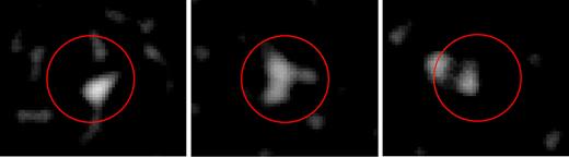
The XMM–Newton EPIC PN images, smoothed with a 5-pixel FWHM 2D Gaussian, are shown in the 0.5–2, 2–5, and 5–10 keV bands. SDSSJ1652 is centred with the circular 15-arcsec extraction region indicated. The photometry is shown in Table 2.
Aperture photometry results of the XMM–Newton and NuSTAR observations in different energy bands.
| Detector | GTI exposure time | Net counts | Count rate | Net counts | Count rate | Net counts | Count rate |
|---|---|---|---|---|---|---|---|
| XMM–Newton | (0.5–2 keV) | (2–5 keV) | (5–10 keV) | ||||
| EPIC MOS-1 | 52020 | 10 ± 5 | 1.8 × 10⁻⁴ | <10 | <2 × 10⁻⁴ | <10 | <2 × 10⁻⁴ |
| EPIC MOS-2 | 46400 | 6 ± 5 | 1.3 × 10⁻⁴ | 7 ± 4 | 1.6 × 10⁻⁴ | <11 | <2 × 10⁻⁴ |
| EPIC PN | 48870 | 15 ± 10 | 3.1 × 10⁻⁴ | 33 ± 9 | 6.8 × 10⁻⁴ | <24 | <5 × 10⁻⁴ |
| NuSTAR | (6–10 keV) | (10–40 keV) | (40–79 keV) | ||||
| FPMA | 218600 | 22 ± 9 | 1 × 10⁻⁴ | 25 ± 18 | 1 × 10⁻⁴ | <48 | <2 × 10⁻⁴ |
| FPMB | 218600 | <31 | <1 × 10⁻⁴ | <54 | <3 × 10⁻⁴ | <45 | <2 × 10⁻⁴ |
Notes. XMM–Newton source counts were extracted from 15-arcsec apertures; and the NuSTAR source counts were extracted from 30-arcsec apertures. The EPIC detectors showed lower signal-to-noise ratio towards the harder bands compared to that of the PN detector. Of the two NuSTAR detectors, only FPMA showed real detections, so we show 3 σ upper limits for FPMB. The 3 σ upper limits are also shown for other bands with low counts. Only data from the EPIC and FPMA detectors were used for the spectral analysis. The Good Time Interval (GTI) exposure time is in seconds.
2.2 NuSTAR
The NuSTAR (Harrison et al. 2013) observatory is the first focusing satellite with sensitivity over a broad high-energy 3–79 keV energy band. It consists of two focal-plane modules (FPMA and FPMB) with a 12×12 arcmin2 field of view. Since we expected low-photon detections due the predicted Compton-thick nature of the SDSSJ1652, a much longer 218-ks observation was performed with NuSTAR on 2019 February 23 (obsID: 60401028002). The NuSTAR data were reduced with the NuSTAR Data Analysis Software (nustardas) v20160502 and the NuSTAR Calibration Database (caldb), using the nupipeline tasks. The spectra and light curves were extracted with the nuproducts task.
Photometry results in Table 2 were extracted from a 30-arcsec radius circular region centred on the target coordinates from both detectors. Despite the long exposure, the FPMB detector did not detect any significant signal from the source. Thus, we only use data from the FPMA detector for spectral analysis. We calculate the 3σ upper limit for FPMB in three bands: 6–10, 10–40, and 40–79 keV. The NuSTAR photometry results are shown in Table 2. The non-detection can be attributed to a few reasons: high attenuation of X-ray signals due to the obscuring material, limited exposure time, and stray light, which complicated background subtraction.
3 X-RAY SPECTRAL ANALYSIS
We perform spectral analysis on SDSSJ1652 with Xspec v12.10 (Arnaud 1996) for photon-limited Cash statistics (Cash 1979). We adopt the Galactic absorption column density of NH, Gal = 5.03 × 1020 cm−2 (HI4PI Collaboration et al. 2016), which is modelled by the phabs Xspec model. We perform simultaneous spectral analysis on the XMM–Newton EPIC (MOS and PN) between 0.5 and 10 keV and the NuSTAR FPMA data between 6 and 79 keV, excluding the FPMB data due to low signal. The objectives are to constrain the power-law photon index Γ associated with the intrinsic luminosity and the column density NH to understand the geometry and scale of the obscuration. All fits are performed in the rest frame assuming z = 2.94.
3.1 Absorbed power-law model
We first fit the SDSSJ1652 spectra with a power-law. The initial fit produces a small photon index Γ ∼ 0.8. Since the typical value of the power-law slopes measured in active galactic nuclei is Γ ≈ 2 (Nandra & Pounds 1994; Reeves & Turner 2000; Page et al. 2005; Piconcelli et al. 2005), the flat spectral slope of Γ ∼ 0.8 is unlikely to reflect the intrinsic properties of the source, but rather indicates the presence of significant absorption (Alexander et al. 2001). The resulting observed spectrum is harder than the intrinsic spectrum of an unobscured quasar (Nandra & Pounds 1994; Goulding et al. 2018).
Next, we model the spectra using a power-law with photoelectric absorption in the rest frame. We refer to this as the absorbed power-law model, and the corresponding Xspec model is listed in Table 3. When all model parameters (column density NH, normalization Knorm, and the photon index Γ) are set as free parameters, the best-fitting model also produce a low power-law index Γ ∼ 0.8, which is likely due to the high soft-energy excess, hinting complex attenuation mechanism. Instead, we adopt the approach taken by Goulding et al. (2018), among others, and force a more physically motivated model. We fix the photon index at a typical slope of Γ = 1.9 and freely fit for the column density NH and energy normalization Knorm. The observed spectra with the best-fitting model are shown in Fig. 2. The best-fitting parameters are |$N_{\rm H}=(9^{+4}_{-3})\times 10^{23}\textrm {~cm}^{-2}$| and Knorm = (6 ± 2) × 10−5 photon keV cm−2 s−1 at 1 keV with an improved Cstat = 633 for 693 degrees of freedom (d.o.f.). The confidence ranges of the calculated NH and Knorm are produced with the Xspec steppar routine. The confidence contours of NH and Knorm fits are shown in Fig. 2. The power-law model with Γ = 1.9 yields the same results for the intrinsic luminosity whether it is applied to just the NuSTAR data or to the combined XMM–Newton+NuSTAR data set. Spectral fit results are summarized in Table 4.
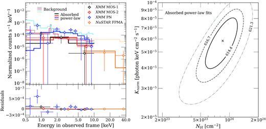
Top left-hand panel: The XMM–Newton and NuSTAR spectra and the folded absorbed power-law model fits are shown. The spectra have been rebinned for plotting purposes. The binned data points are indicated with circles, and the models are shown as solid lines: MOS-1 (black), MOS-2 (red), PN (blue), and FPMA (orange). The extracted background spectrum for each detectors are also shown as faded lines in the same colour scheme. Bottom left-hand panel: The data-model residuals show increased deviations in the <1.5 keV soft-energy region, which indicates the need for a more complex model. While it is possible that the soft-energy features may be background driven, it is unlikely that features around 3–5 keV are affected by the background. Right-hand panel: The confidence contours for the best-fitting Knorm and NH for the absorbed power-law model. The contour lines represent the 68 (solid), 90 (dashed), and |$99{{\ \rm per\ cent}}$| (dash–dotted) Cstat confidence levels for 693 degrees of freedom. We see that the model indicates a near-Compton thick absortion of NH ∼ 1024 cm−2.
The Xspec commands for each model considered.
| Model | Xspec commands |
|---|---|
| Absorbed power-law | phabs*zphabs*zpowerlw |
| MYTorus | const1*phabs(zpowerlw*MYTZ + const2*MYTS + const3*gsmooth*MYTL + const4*zpowerlw) |
| Model | Xspec commands |
|---|---|
| Absorbed power-law | phabs*zphabs*zpowerlw |
| MYTorus | const1*phabs(zpowerlw*MYTZ + const2*MYTS + const3*gsmooth*MYTL + const4*zpowerlw) |
Notes. A constant Galactic absorption (phabs) is assumed for both models. The MYTorus model describes a reprocessed spectrum (MYTZ, MYTS, and MYTL) and an optically thin scattered continuum, assuming a terminal energy of 500 keV. Normalization for the Compton scattered emission (const2) and fluorescent line emission (const3) are tied together for a self-consistent model. The scattering fraction fsc is given by const4, which is linked to the power-law model of the source zpowerlw.
Best-fitting parameters for the unabsorbed power-law, absorbed power-law model, and the MYTorus models at varying θi.
| Parameter | Power-law | Absorbed power-law | MYTorus | ||||
|---|---|---|---|---|---|---|---|
| θi = 45° | 60° | 75° | 85° | ||||
| Γ | – | 0.8 ± 0.3 | (1.9) | (1.9) | (1.9) | (1.9) | (1.9) |
| Knorm | (10−5 photons keV−1 cm−2 s−1) | |$0.1^{+0.2}_{-0.1}$| | 6 ± 2 | |$0.3^{+0.3}_{-0.9}$| | |$0.9^{+0.3}_{-0.9}$| | |$8^{+7}_{-4}$| | |$9^{+7}_{-4}$| |
| NH | (1024 cm−2) | – | |$0.9^{+0.4}_{-0.3}$| | 2 ± 52 | 2 ± 27 | |$1.2^{+1}_{-0.5}$| | 1.02|$^{+0.76}_{-0.41}$| |
| fsc | (10−2) | – | – | 3 ± 20 | 1 ± 4 | 3.5 ± 2.8 | 3.6 ± 2.7 |
| C-stat | (d.o.f.) | 617 (665) | 633 (693) | 656 (692) | 655 (692) | 610 (664) | 610 (667) |
| L2–10, obs | (1044 erg s−1) | – | |$0.7^{+0.2}_{-0.2}$| | |$1^{+2}_{-0.9}$| | |$1^{+4}_{-0.9}$| | |$0.9^{+0.3}_{-0.2}$| | |$0.9^{+0.2}_{-0.3}$| |
| L2–10, int | (1045 erg s−1) | |$0.11^{+0.01}_{-0.05}$| | |$0.6^{+0.4}_{-0.2}$| | |$2.5^{+2}_{-1}$| | 0.9 ± 0.9 | 1.2 ± 1 | 1.4|$^{+1}_{-1}$| |
Notes. The power-law index is fixed at Γ = 1.9 for all models with absorption. For the detailed error bounds, refer to the confidence contours in Figs 2 and 3 for the absorbed power-law and the MYTorus models, respectively. L2–10, obs indicate observed luminosity, and L2–10, int indicate absorption-corrected luminosity, both in rest frame. All parameters have been redshift corrected. Stated uncertainties represent the 90 per cent confidence interval.
The best-fitting model spectrum in Fig. 2 displays a noticeable inversion around the observed frame 1.5 keV. Examining the data-model residual, we see that this absorbed power-law model does not capture this observed-frame soft-energy excess in the 0.5–1 keV range. Although the Fe K α emission line (1.6 keV in the observed frame) is present (Piconcelli et al. 2015), due to the low counts observed, we cannot find an appropriate binning that comfortably shows both the line and the continuum. These observed spectral features combined with the initial column density estimate approaching NH ∼ 1024 cm−2 suggest significant Compton-thick obscuration with a more complex absorption structure.
3.2 MYTorus model
We adopt the physically motivated MYTorus spectral model (Murphy & Yaqoob 2009; Yaqoob 2012), which is a Monte Carlo model based on a toroidal circumnuclear reprocessor that also accounts for geometry. The increased soft X-ray component seen in Fig. 2 suggests a Compton scattering continuum, which MYTorus can also model self-consistently. We fit a model that uses pre-calculated MYTorus tables that include: (a) the zeroth-order reprocessed power-law continuum – MYTZ, (b) the Compton-scattered continuum – MYTS, (c) the scattered fluorescent line emission due to Fe K at ∼6.4-keV rest frame – MYTL, and (d) the optically-thin scattered power-law continuum, separate from the MYTorus tables, to account for electron scattering in a warm/hot ionized region surrounding the central engine. This added optically-thin scattering region is larger than the obscuring structure. For simplicity, we refer to this model set as the MYTorus model throughout this paper. This spectral shape is motivated by the stacked analysis in Goulding et al. (2018). The Xspec implementation of this model is shown in Table 3. All models considered assume that the intrinsic power-law continuum terminates at 500 keV, referred to as the terminal energy.
Similar to the absorbed power-law model treatment, we fix Γ = 1.9 and tie it to each MYTorus model components. We also fix the MYTorus normalization constants at unity and link each of their column densities NH. Previous UV spectropolarimetry analysis suggested a broad-line region scattering, in which the likely line-of-sight inclination angle θi to the central engine is near edge-on; however, θi was not constrained at the time (Alexandroff et al. 2018). Rather than treating θi as another free parameter, we fix at a particular value, and freely fit for Knorm, NH, and the scattering fraction fsc corresponding to the optically-thin scattered continuum. We repeat this fitting process over four angles: θi = 45°, 60°, 75°, and 85° (edge-on is defined as 90°). In each iteration of the fit, we initially fix |$f_{\rm sc}=1{{\ \rm per\ cent}}$| to localize NH, then free the fsc parameter for simultaneous Knorm, NH, and fsc fitting.
The best-fitting parameters for the four MYTorus models are listed in Table 4, and the corresponding confidence contour maps of the NH and fsc fits are shown in Fig. 3. We find a strong dependence on θi, in which greater inclination angles are preferred. In fact, the uncertainties for the θi = 45° and 60° could not be constrained, reaching extreme estimates for NH and fsc as indicated by the |$68 {{\ \rm per\ cent}}$| contour. From the fit values and the contour maps, we conclude that the θi = 75° and 85° geometries fit the data better. Since the estimated values for NH and fsc at these two angles are nearly identical with overlapping error bounds, it is difficult to conclusively pick one model over the other. Neither were we able to constrain a lower limit for fsc to high confidence. However, the confidence contour maps in Fig. 3 suggest that the model parameters are better constrained at θi = 85° with NH = (1.02|$^{+0.76}_{-0.41}$|) × 1024 cm−2 and fsc = (3 ± 2) per cent at |$90 {{\ \rm per\ cent}}$| confidence with Cstat = 610 for 667 degrees of freedom.
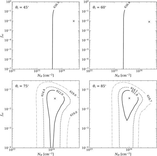
The confidence contours for the best-fitting MYTorus parameters NH and fsc for θi = 45° (top left-hand panel), 60° (top right-hand panel), θi = 75° (bottom left-hand panel), and 85° (bottom right-hand panel) at 68 (solid), 90 (dashed), and 99 per cent (dash–dotted) Cstat confidence levels. It was not possible to constrain the confidence contours better than |$68 {{\ \rm per\ cent}}$| for θi = 45° (left-hand panels) and 60°. Comparing the contours, we find that larger inclinations are preferred; and the θi = 85° model appear to better constrain NH and fsc over θi = 75° .
The unfolded energy spectrum with the best-fitting θi = 85° MYTorus model is shown in Fig. 4. We compare the different best-fitting unfolded MYTorus θi models with the observed data. We also plot the models and their respective components in Fig. 4. Despite the differences in fits, all of the MYTorus model fit results suggest that SDSSJ1652 is a highly obscured, Compton-thick quasar. The calculated model (redshift and absorption-corrected) rest-frame luminosity for the θi = 85° model is L2–10= (1.4|$^{+1}_{-1}$|) × 1045 erg s−1.
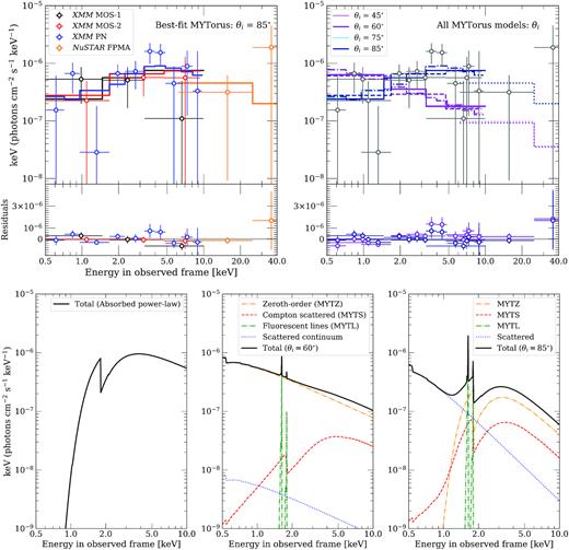
Top left-hand panel: the observed-frame, unfolded energy spectrum with the best-fitting θi = 85° MYTorus model. The spectra have been re-binned for plotting purpose. The binned data points are shown in circles, and the black, red, blue, and orange solid lines represent the best-fitting MYTorus model at θi = 85°. Top right-hand panel: all of the MYTorus models for the various θi considered are plotted against the binned data points (in grey). The data-model residuals in units of keV are also shown and show that models at larger θi (light/dark blue) capture both the soft- and hard-energy data better than at smaller θi (light/dark purple). Bottom panel: comparison of the observed frame absorbed power-law (left-hand panel) and MYTorus models, θi = 60° (centre panel) and 85° (right-hand panel), with the power-law parameter fixed at Γ = 1.9. The solid black line indicates the total model spectrum, while the coloured dashed/dotted lines indicate the individual model components. We note that a pure absorbed power-law does not capture the soft-energy components, while the less inclined MYTorus θi = 60° spectrum predicts a smoother profile without a prominent hard Compton-scattered continuum past the Fe K α fluorescent line, suggesting a highly inclined geometry such as the θi = 85° model. Refer to Table 4 for the best-fitting parameters of each model.
3.3 Comparing the models
The C-stat values of the best fitting the absorbed power-law and MYTorus models both indicate similar goodness-of-fits. Here we focus on the data-model residuals in Figs 2 and 4. In general, the MYTorus model fits capture the spectral features across all energies better than absorbed power-law model (Fig. 2 left-hand panel versus Fig. 4 top left-hand panel). We argue that the MYTorus model fit is mostly driven by the spectral shape in E > 2 keV observed frame. In fact, according to just the C-stat values, the θi = 45° and 60° MYTorus models would be preferred over the θi = 75° and 85° models, which is not supported by the parameter confidence contours. An obscuring structure with a more inclined geometry is preferred to explain the medium/hard energies.
However, there are some uncertainties within the MYTorus model fits that do not fully model the spectral features at <1.5 keV and 3–5 keV, which are more pronounced in the XMM–Newton/PN data (blue data points). The background spectrum in Fig. 2 does not show any significant features at 3–5 keV, suggesting that the unmodelled features are not likely to be background driven. Unmodelled components in 3–5 keV may suggest that we are not fully modelling the peak of the X-ray emission, implying underestimated NH, L2–10, and fsc.
To understand the soft-energy fits, we also considered MYTorus models without the warm electron scattering, which produce similar best-fitting θi, NH, Knorm, and C-stat values. With this modification, the best-fitting spectrum displays deviations in the soft-energies similar to that of the absorbed power-law model, suggesting the need for a soft-energy scattering component. Therefore, we argue that the inclined MYTorus geometry with the scattering region is the preferred model. A possible explanation for the systematic model residuals in our best-fitting MYTorus model is a presence of a more complex thermal structure, not captured by MYTorus or the electron scattering components. However, adding a thermal component did not change the parameters nor improve the fit quality, so we cannot preferentially constrain the model. Another possibility is a presence of a more complex obscuring torus that can be described with a variable opening angle model like borus (Baloković et al. 2018) as explored in LaMassa et al. (2019), but this would require higher signal data. Finally, the remaining uncertainties may reflect the poor data quality from severely photon-limited studies.
4 DISCUSSION
4.1 Power of central engine
There is an ongoing debate about the relationship between outflows and accretion in luminous quasars: whether near-Eddington accretion is associated with disrupting the X-ray-emitting corona or whether the corona must be compact and shielded to enable radiative driving (Luo et al. 2013). The X-ray luminosity is one of the key determinants of the wind launching mechanism.
X-ray emission and mid-infrared emission are both tracers of black hole accretion activities. X-rays originate from the corona over the inner accretion flow and the mid-infrared emission is re-radiated by the obscuring dust on larger scales. A common analysis is to compare the intrinsic 2–10 keV X-ray luminosity, L2–10, against the mid-infrared rest-frame 6-μm luminosity, L6 μm. Stern (2015) and Chen et al. (2017) showed an empirically derived sub-linear L6 μm–L2–10 relationship for luminous Type I quasars with L6 μm ≳ 1045 erg s−1, in which the measured L2–10 at fixed L6 μm is an order of magnitude below the extrapolations expected from the linear Gandhi et al. (2009) relationship, as shown in Fig. 5. The origin of this sub-linear relationship remain unresolved.
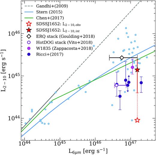
The L6 μm–L2–10 relationships for selected targets, including SDSSJ1652 are shown. All L2–10 indicate the absorption corrected, intrinsic X-ray luminosities, unless otherwise noted. Since the original linear relation by Gandhi et al. (2009) was derived for L12 μm < 1045 erg s−1, the extrapolated relation at higher luminosities, corrected for L6 μm, is shown as a dashed grey line. Sublinear relationships derived for higher luminosities by Stern (2015) and Chen et al. (2017) are shown as solid blue and green lines; the blue data points correspond to Type I quasars used in Stern (2015). The observed (open star) and intrinsic (filled star) L2–10 of SDSSJ1652 using the MYTorus model is shown with 90 per cent confidence. The stacked ERQ (Goulding et al. 2018) result is shown with the error bars spanning the observed L6 μm range. Both the stacked ERQ and SDSSJ1652 results are consistent with the relationships derived for Type I quasars. We also compare selected hot dust-obscured galaxy (HotDOG) results (Ricci et al. 2017), including stacked analysis showing low L2–10 (Vito et al. 2018) and a deep observation of W1835+4355 with high L2–10 (Zappacosta et al. 2018).
One possibility is that luminous quasars with strong X-rays would overly ionize the circumnuclear gas and suppress the production of radiatively-driven winds (Luo et al. 2013). The physical connection would then lead to the observed Stern (2015) and Chen et al. (2017) relations through the coronal quenching phenomenon (Luo et al. 2013), in which X-ray emission is suppressed by a massive accretion flow such as a failed disc wind that falls into the accretion disc (Proga 2005; Leighly et al. 2007; Lusso et al. 2010; Jin, Ward & Done 2012). This would suggest that high accretion efficiency leads to a decrease in radiative efficiency.
Interestingly, there is evidence for other luminous quasars with even weaker observed X-ray luminosities, falling below the Stern (2015) and Chen et al. (2017) relations even after accounting for absorption (Lansbury et al. 2020). Examples of quasars with a very weak X-ray emission include a Type I quasar with emission-line outflows (Leighly et al. 2007), BAL quasars (Luo et al. 2013), ultraluminous infrared galaxies (ULIRGs; Teng et al. 2014, 2015), and HotDOGs (Ricci et al. 2017). Either these quasars are intrinsically X-ray weak or they have a complex inner geometrical structure with multiple absorbers that cannot be identified in a single low-quality spectrum.
Combining the WISE photometry data and the X-ray analysis from this paper, we can perform a similar analysis to probe the outflow mechanisms of SDSSJ1652. In Fig. 5, we compare the results for SDSSJ1652 against the Stern (2015) and Chen et al. (2017) relationships and the stacked Chandra measurements of ERQs, which includes SDSSJ1652, by Goulding et al. (2018). Given the uncertainties of individual sources using the stacking technique, the stacking estimate and our estimate of the intrinsic luminosity of SDSSJ1652 are consistent, while deeper observations of SDSSJ1652 places a better constraint on the absorption-corrected luminosity. This result supports the Goulding et al. (2018) observation that there is no strong evidence that ERQs are intrinsically X-ray weak. They appear to be consistent with Type I quasars once the intervening absorption is accounted for. These results would suggest that despite the presence of extreme outflows, the heavily obscured SDSSJ1652 and other ERQs are not dominated by extreme coronal quenching that would otherwise result in extreme X-ray suppression, hence they are not intrinsically X-ray weak.
It is also possible for the measured L6 μm to be underestimated due to obscuration or due to anisotopic emission (Zappacosta et al. 2018), which would imply L2–10 deficit compared to the standard relationships and strong X-ray suppression. This would require a correction of nearly an order of magnitude to impose a significant departure from the observed L6 μm–L2–10 relationship, which is unlikely. Goulding et al. (2018) notes that the observed high luminosities and outflows in ERQs may be due to a combination of colour selection and orientation effects. Current observations of SDSSJ1652 and other ERQs suggest that they are dissimilar from X-ray weak BAL quasars in Luo et al. (2013) in terms of their relationship between extreme accretion, coronal quenching, and outflows. Therefore, it is possible that the ERQs have an outflow mechanism that is different from those of BAL quasars.
4.2 Obscuration properties
The obscuration geometry of the best-fitting MYTorus model is broadly comprised of two components: the obscuring torus and optically-thin scattering region. The θi = 85° MYTorus result is consistent with the near-edge-on line-of-sight geometry described by Alexandroff et al. (2018), which suggest the observed X-ray absorption must occur in same wind as the observed UV scattering (Goulding et al. 2018). In the Alexandroff et al. (2018) model, the polarized UV wind in SDSSJ1652 is likely due to dust scattering somewhere in the broad emission-line region (BELR) and broad absorption-line region (BALR) at scales greater than the obscuration. The inclined viewing angle inferred in the UV is based on the observed shape of the infrared SED. With the inclusion of the X-ray results, our MYTorus model fits adds the absorbing torus and the warm/hot ionized electron scattering region surrounding the central engine. A cartoon picture of the combined SDSSJ1652 model is shown in Fig. 6.
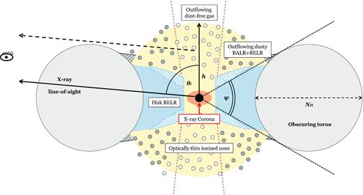
This diagram (not to scale) shows the preferred model picture for SDSSJ1652 adapted from Alexandroff et al. (2018) and combined with our best-fitting X-ray MYTorus model parameters described in Table 4. The reprocessed MYTorus model flux is shown in solid black line, and the scattered flux is in dashed line. This illustrates the cross-sectional view through obscuring torus. The model is inspired by Veilleux et al. (2016). The inner accretion disc is surrounded by a geometrically thick BELR accretion disc (in light blue), in which scattering of the dusty equatorial outflow that produces UV-polarization occurs higher in the dusty BALR and BELR. The torus (in grey) geometry is adapted from Murphy & Yaqoob (2009), which assumes a half-opening angle of ψ = 60° (equivalent to a covering factor of ΔΩ/4π = 0.5). The best-fitting MYTorus model suggest a highly inclined near edge-on geometry of θi = 85°. Our model describes the X-ray power-law continuum experiencing photoelectric absorption, Compton-scattering, and electron scattering from the warm/hot ionized region surrounding the central engine (in yellow).
The optically-thin scattered power-law continuum is commonly observed as a rise in the X-ray spectrum towards the low energies. The scattered spectrum is assumed to have the same shape (i.e. Γ) as the incident power-law spectrum and is assumed to be due to electron scattering. This means that the scattering fraction fsc is the ratio of the scattered flux to the incident flux. This extended scattering region needs to be on scales larger than the central engine and the obscuring torus, which, in turn, must be larger than the derived dust sublimation region. Using the dust sublimation estimate (Barvainis 1987) and the extrapolated UV luminosity, we find that the dust sublimation distance is ∼1 pc (Alexandroff et al. 2018).
4.3 Nature of the SDSSJ1652
We calculate the order-of-magnitude approximations for the central black hole accretion properties. The directly observed L6 μm of 1047.19 erg s−1 suggests that the bolometric luminosity may be of the order LBol ∼ 1047–48 erg s−1, which is in agreement with the Perrotta et al. (2019) measurement of LBol ∼ 1047.73 erg s−1. This would correspond to a X-ray bolometric correction κX ≈ 380 for LBol = κXL2–10, obs. This is roughly in agreement with values found for z = 2–4 hyperluminous Type I quasars (Martocchia et al. 2017).
While there are many scaling relationships for black hole mass MBH measurements (e.g. host stellar mass, H β kinematics), there are many caveats that complicate direct comparison to ERQs, as noted by Zakamska et al. (2019). Without reliable X-ray to MBH scaling relations, it is also difficult to independently measure MBH from this study. With this in mind, we consider the H β virial mass estimate of the SDSSJ1652 supermassive black hole by Perrotta et al. (2019): |$M_{\rm BH}=3\times 10^9\,{\rm M}_{\odot}$|, which corresponds to an Eddington luminosity of LEdd = 4 × 1047erg s−1. Combined with the Perrotta et al. (2019) bolometric luminosity, the Eddington ratio is estimated to be LBol/LEdd ∼ 1.2. Zakamska et al. (2019) explained that a possible argument against high Eddington ratios is an overestimated LBol. However, for obscured populations, underestimated LBol is more likely especially when the observed L6 μm–L2–10 relationship is consistent with Stern (2015) and Chen et al. (2017). Therefore, SDSSJ1652 is consistent with being a near- or super-Eddington, Compton-thick source, exhibiting high L2–10 and powerful outflows.
4.4 Comparing with other observations
While there are X-ray studies of highly obscured quasars, most have been limited to low-redshift samples. Another class of reddened quasars are the HotDOGs, which have properties similar to those of ERQs in terms of spectral energy distribution, luminosity, and redshift (Eisenhardt et al. 2012; Assef et al. 2015). Despite these similarities, there are some interesting differences stemming from somewhat different selection methods. One such difference is that HotDOGs are well below the Stern (2015) and Chen et al. (2017) relationships (Ricci et al. 2017; Vito et al. 2018), while also showing Compton-thick obscurations (Piconcelli et al. 2015), in contrast to ERQs explored in Goulding et al. (2018) and in this paper. We compare their L6 μm–L2–10 properties in Fig. 5.
A recent NuSTAR observation of a z = 2.298 HotDOG (W1835+4355) showed Compton-thick obscuration, NH ≈ 0.9 × 1024 cm−2, and absorption-corrected luminosity of L2–10 = 1.6 × 1045 erg s−1 (Zappacosta et al. 2018) similar to those of SDSSJ1652 presented here. Compared to other HotDOGs, this target also exhibited higher X-ray luminosity, nearly consistent with the Stern (2015) and Chen et al. (2017) relations, shown in Fig. 5. In contrast to SDSSJ1652, their target was modelled with θi = 70° and a larger model-dependent |$f_{\rm sc}\approx 5\!-\!15{{\ \rm per\ cent}}$|. This suggest remarkable similarities between ERQs and HotDOGs with the only differences in the obscuration properties: θi and fsc. This indicates a variety in HotDOG properties with some that have overlapping L6 μm–L2–10 properties to ERQs.
5 CONCLUSION
We report on deep ∼ 130-ks XMM–Newton and ∼ 218-ks NuSTAR observations of SDSSJ1652, an obscured, extremely red quasar at z = 2.94. We characterize the intrinsic X-ray properties and obscuration geometry using XMM–Newton, which is sensitive to the absorbing column, and NuSTAR, which probes the intrinsically unobscured X-rays. We determine the accretion luminosity and the obscuration properties of SDSSJ1652 to provide verification for severely photon-limited studies of the high-redshift, obscured quasar population.
We extracted spectra from the XMM–Newton MOS and PN and the NuSTAR FPMA detectors. Unfortunately, we could only place a 3σ upper limit for the NuSTAR FPMB. We fit 0.5–10 keV XMM–Newton and 6–79 keV NuSTAR spectra with a physically motivated MYTorus model that models the zeroth-order continuum reprocessing due to the intervening cold gas, Compton-scattered continuum, fluorescent line emission, and the optically-thin scattered power-law continuum due to electron scattering in the warm ionized region surrounding the central engine. We find the best-fitting model indicates a Compton-thick column density of NH = (1.02|$^{+0.76}_{-0.41}$|) × 1024 cm−2, a near edge-on geometry with the line-of-sight inclination angle of θi = 85°, and a warm electron scattering fraction of |$f_{\rm sc}\sim 3{{\ \rm per\ cent}}$|.
From the measured obscuration parameters, we place estimates of the physical properties of the obscuration, assuming scale heights h ∼ 1–10 pc for dust and electron scattering. From fsc, we estimate the electron density driving the soft-energy scattering to be in the range ne ∼ 7.5 × (102–103) cm−3. From NH, we estimate the obscuration mass to be approximately |$M_{\rm obsc}\sim 1.7\times (10^4\!-\!10^6)\,{\rm M}_{\odot}$|. These values are highly uncertain due to uncertainties in the torus geometry.
The absorption-corrected, intrinsic X-ray luminosity is L2–10= (1.4|$^{+1}_{-1}$|) × 1045 erg s−1. This is consistent with the L6 μm–L2–10 relationship for luminous Type I quasars, which indicates that SDSSJ1652 is not X-ray weak once corrected for the Compton-thick absorption. This trend is consistent with other ERQs, in contrast to other known luminous quasars. The observed L6 μm–L2–10 would imply that SDSSJ1652 may not be experiencing coronal quenching that would nominally suppress X-ray radiation supposedly associated with high accretion. Moreover, the observed luminosity estimates support the energetics needed to drive the observed galactic scale outflows. These results indicate the ability of near- or super-Eddington, Compton-thick ERQs like SDSSJ1652 to drive powerful outflows without requiring intrinsically weak X-rays.
ACKNOWLEDGEMENTS
This research was supported by NASA grant NuSTAR GO-4298. This research is based on observations obtained with XMM–Newton, an ESA science mission with instruments and contributions directly funded by ESA Member States and NASA. This research has made use of data obtained with NuSTAR, a project led by Caltech, funded by NASA and managed by NASA/JPL, and has utilized the nustardas software package, jointly developed by the ASDC (Italy) and Caltech (USA). This research has made use of data and/or software provided by the High Energy Astrophysics Science Archive Research Center (HEASARC), which is a service of the Astrophysics Science Division at NASA/GSFC.
We also thank the referee for the valuable feedback and comments in improving this paper.
DATA AVAILABILITY
The data underlying this paper are already available in the HEASARC Archives at https://heasarc.gsfc.nasa.gov/docs/archive.html and the XMM–Newton Science Archives at http://nxsa.esac.esa.int/ and can be accessed with the corresponding ObsID.
