


ABSTRACT
Building accurate and flexible galaxy–halo connection models is crucial in modelling galaxy clustering on non-linear scales. Recent studies have found that halo concentration by itself cannot capture the full galaxy assembly bias effect and that the local environment of the halo can be an excellent indicator of galaxy assembly bias. In this paper, we propose an extended halo occupation distribution (HOD) model that includes both a concentration-based assembly bias term and an environment-based assembly bias term. We use this model to achieve a good fit (χ2/degrees of freedom = 1.35) on the 2D redshift-space two-point correlation function (2PCF) of the Baryon Oscillation Spectroscopic Survey (BOSS) CMASS galaxy sample. We find that the inclusion of both assembly bias terms is strongly favoured by the data and the standard five-parameter HOD model is strongly rejected. More interestingly, the redshift-space 2PCF drives the assembly bias parameters in a way that preferentially assigns galaxies to lower mass haloes. This results in galaxy–galaxy lensing predictions that are within 1σ agreement with the observation, alleviating the perceived tension between galaxy clustering and lensing. We also showcase a consistent 3σ–5σ preference for a positive environment-based assembly bias that persists over variations in the fit. We speculate that the environmental dependence might be driven by underlying processes such as mergers and feedback, but might also be indicative of a larger halo boundaries such as the splashback radius. Regardless, this work highlights the importance of building flexible galaxy–halo connection models and demonstrates the extra constraining power of the redshift-space 2PCF.
1 INTRODUCTION
In the standard framework of structure formation in a Λ cold dark matter (ΛCDM) universe, galaxies are predicted to form and evolve in dark matter haloes (White & Rees 1978). While the distribution and structure of dark matter haloes are directly tied to the underlying cosmology, the extent to which galaxies do is less so. To extract cosmological information and understand galaxy formation from observed galaxy clustering statistics, it is critical to correctly model the connection between galaxies and their underlying dark matter haloes. The most popular model of the galaxy–halo connection is the halo occupation distribution (HOD) model (e.g. Peacock & Smith 2000; Scoccimarro et al. 2001; Berlind & Weinberg 2002; Zheng et al. 2005; Zheng, Coil & Zehavi 2007). The HOD makes the assumption that all galaxies live inside dark matter haloes, and expresses the average number of galaxies contained within an individual halo as a function of the halo mass. More specifically, the simplest formulation of the HOD assumes that galaxy occupation is determined solely by halo mass, an assumption that rests on the long-standing and widely accepted theoretical prediction that halo mass is the attribute that most strongly correlates with the halo abundance and halo clustering and the properties of the galaxies residing in it (White & Rees 1978; Blumenthal et al. 1984).
However, Gao, Springel & White (2005), Zentner et al. (2005), Wechsler et al. (2006), Gao & White (2007), Croton, Gao & White (2007), and Li, Mo & Gao (2008) showed that at fixed halo mass, halo clustering also depends on secondary halo properties that correlate with halo assembly history, an effect known as halo assembly bias. Additionally, a series of studies employing hydrodynamical simulations and semi-analytic models have found clear evidence that galaxy occupation correlates with secondary halo properties beyond just halo mass (e.g. Zhu et al. 2006; Artale et al. 2018; Zehavi et al. 2018; Bose et al. 2019; Contreras et al. 2019; Hadzhiyska et al. 2020; Xu, Zehavi & Contreras 2021). This phenomenon is commonly known as galaxy assembly bias (or assembly bias hereafter) to differentiate it from halo assembly bias. Wechsler & Tinker (2018) offer a more rigorous definition of assembly bias as: at fixed halo mass, the galaxy properties or number of galaxies within dark matter haloes may depend on secondary halo properties that themselves show a halo assembly bias signature. Ignoring the effects of assembly bias has been shown to introduce significant errors in inferring galaxy–halo connection models and bias galaxy formation models (Pujol & Gaztañaga 2014; Zentner, Hearin & van den Bosch 2014; Lange et al. 2019).
Several studies have implemented ways to incorporate a secondary dependence into the HOD formalism (e.g. Paranjape et al. 2015; Hearin et al. 2016; McEwen & Weinberg 2018; Yuan, Eisenstein & Garrison 2018; Walsh & Tinker 2019; Wibking et al. 2019; Xu et al. 2021). The different methodologies can be summarized into two approaches. One approach is to assign galaxies to haloes according to a secondary property within each mass bin, such as the decorated HOD framework proposed in Hearin et al. (2016). The other approach is to introduce a secondary dependence on the existing HOD parameter set, but where the definition of halo mass itself is modified by a dependence on the secondary parameter, such as in Yuan et al. (2018) and Walsh & Tinker (2019). Zentner et al. (2019) applied the decorated HOD framework showed the first tentative observational evidence for galaxy assembly bias in the Sloan Digital Sky Survey (SDSS) Data Release 7 (DR7) main galaxy sample.
Thus far, halo concentration, which is a measure of how centrally peaked the density profile of the halo is, has long been regarded as the standard secondary parameter to use in assembly bias studies. This choice is largely motivated by N-body simulations that show that halo concentration, along with several other parameters that correlate with the halo assembly history, is good predictors of halo assembly bias (Wechsler et al. 2006; Croton et al. 2007; Mao, Zentner & Wechsler 2018). However, recent studies that have systemically compared various secondary dependencies for assembly bias in hydrodynamical simulations and semi-analytic models have found that halo concentration only accounts for part of the actual assembly bias (Hadzhiyska et al. 2020; Xu et al. 2021). Both studies find that the local environment of the halo at the present day is an excellent predictor of assembly bias, where the environment is defined as either the smoothed local matter density or the number of neighbouring haloes within some radius. We point out that the term ‘assembly bias’ is somewhat of a misnomer in this context, as dependencies such as local environment identified today do not necessarily relate to the past assembly history of the haloes. In this paper, we mean assembly bias in its most general sense, inclusive of all secondary dependencies in the galaxy–halo connection model.
However, one must be careful when discussing halo environment in the context of assembly bias, as this may at first seem tautological. Since the environment of the halo is a statement on clustering itself, the halo environment cannot be naively used as the explanation for why there is assembly bias, since it is logically necessary that objects selected from dense environments exhibit stronger clustering. However, if one’s objective is to reproduce realistic galaxy mocks rather than explaining it, then it is fair to use the halo environment as an indicator of assembly bias in decorating galaxy–halo connection models. In fact, as Hadzhiyska et al. (2020) and Xu et al. (2021) have shown, halo environment is potentially the most effective indicator of assembly bias. In the context of dark matter only simulations, halo environment is also powerful because it is an easily accessible property, which bypasses the need to construct halo merger trees or resolve subhalo structure.
There is also growing evidence that halo environment affects galaxy evolution and, therefore, the galaxy–halo connection directly. Both Hadzhiyska et al. (2020) and Xu et al. (2021) showed that while the environment is defined locally (typically between 1 and 5 h−1 Mpc), it seems to capture the assembly bias effects on much larger scales, up to tens of megaparsecs. This suggests that the environment might trace underlying processes that, at least partially, drive assembly bias. This should not be surprising as excursion set theory predicts a correlation between the halo environment and its formation history (Bond et al. 1991; Zentner 2007). In the context of the cosmic web structure, studies have shown that, when controlled for halo mass, galaxy evolution depends on its proximity to close-by cosmic filaments, and the content and kinematics of neighbouring gas reservoirs (e.g. Chen et al. 2017; Poudel et al. 2017; Laigle et al. 2018; Kraljic et al. 2019; Salerno, Martínez & Muriel 2019; Song et al. 2020). Obuljen, Percival & Dalal (2020) found a 5σ detection of an anisotropic assembly bias that correlates galaxy properties with large-scale tidal field in the Baryon Oscillation Spectroscopic Survey (BOSS) CMASS data. A series of papers including Tinker et al. (2017, 2018a,b) studied the relation between various observed galaxy properties and environment at fixed halo mass and stellar mass and found that star-forming galaxies tend to live in underdense environments, whereas quenched passive galaxies tend to occupy overdense environments. Independent studies such as Lee et al. (2018), Dragomir et al. (2018), and Behroozi et al. (2019) found similar trends in simulations and in separate data sets.
In this paper, we propose an extended HOD model that incorporates both a concentration-based assembly bias term and an environment-based assembly bias term. We constrain such an HOD with the observed two-dimensional galaxy redshift-space two-point correlation function (2PCF) of the BOSS (Eisenstein et al. 2011; Dawson et al. 2013) CMASS sample in the range 0.46 ≤ z ≤ 0.6 (Data Release 12). We show that the redshift-space 2PCF strongly prefers the inclusion of both assembly bias terms and affects the fit in a way that reduces the typical host halo mass of galaxies. We also show that the resulting best-fitting HOD predicts the galaxy–galaxy lensing signal to within 1σ, significantly reducing the perceived tension between galaxy clustering and lensing. Our results show that incorporating various galaxy assembly bias effects is an important ingredient in an accurate and flexible HOD model, and that the perceived tension between galaxy clustering and galaxy–galaxy lensing might partially be due to oversimplistic HOD models and the lack of constraining power of the projected 2PCF. We also showcase a consistent preference for a positive environment-based assembly bias by the data. This serves as further evidence that an environment-based assembly bias, together with the traditional concentration-based assembly bias, should be included in future galaxy–halo connection models.
The paper is organized as follows. In Section 2, we describe the extended HOD framework and the implementation of assembly bias parameters. In Section 3, we describe the observed redshift-space 2PCF and the simulation sets we employ in this work. In Section 4, we present the HOD fitting methodology and the optimizations developed for our analysis. In Section 5, we showcase our HOD fits with and without the assembly bias terms, the corresponding lensing predictions, and the best-fitting value of the environment-based assembly bias across variations to the fit. In Section 6, we discuss the parameter recovery of our routine, alternative environment definitions, and compare our assembly bias fit to previous works. We conclude in Section 7.
2 THE EXTENDED HOD FRAMEWORK
The HOD is a popular empirical framework used to populate dark matter haloes with central and satellite galaxies as a function of halo mass. However, given the simplistic nature of galaxy assignment, this model may also be a source of systematic errors for cosmological applications. In this section, we briefly review the baseline HOD formalism and discuss physically motivated extensions to the standard HOD. A more detailed description of the HOD and some of the extensions discussed here can be found in Yuan et al. (2018) and in section 2 of Yuan, Eisenstein & Leauthaud (2020). Our extended HOD code is publicly available as the grand-hod package.1
2.1 The baseline model
In the following subsections, we introduce six additional physically motivated HOD parameters.
2.2 Satellite profile parameters s and sp
We first introduce two parameters that allow for flexibility in the radial distribution of satellite galaxies within each halo.
The radial distance parameter, s, deviates the satellite spatial distribution away from the halo matter density profile by giving preference to particles based on their radial distance to halo centre. A positive s preferentially situates satellites on the outskirts of the halo, whereas a negative s preferentially situates satellites towards the inner region of the halo. Fig. 2 of Yuan et al. (2018) shows how changing s affects the mock 2PCF. The range of s is defined to be between −1 and 1. The s parameter is motivated by baryonic processes that can bias the concentration of baryons within the dark matter potential well (e.g. Abadi et al. 2010; Duffy et al. 2010; Chua et al. 2017; Peirani et al. 2017).
The perihelion distance parameter, sp, is related to the s parameter but additionally folds in the velocity information of the particles. Specifically, it gives preference to particles based on their perihelion distance to the halo centre, i.e. their closest approach distance to the halo centre given their current trajectory. The perihelion distance is calculated by solving the Kepler equations within an NFW potential well (equations 6–9 in Yuan et al. 2018). The impact of sp on the 2PCF is shown in fig. 5 of Yuan et al. (2018). This parameter is motivated by processes such as ram pressure stripping and tidal disruption.
2.3 Velocity bias parameters sv and αc
Another important set of parameters we employ in order to accurately model the redshift-space correlation function is the satellite and central velocity bias parameters (e.g. Berlind et al. 2003; Yoshikawa, Jing & Börner 2003; van den Bosch et al. 2005; Skibba et al. 2011; Guo et al. 2015).
First, we define the satellite velocity bias parameter, sv, which biases the satellite velocity distribution away from that of the host halo. A positive sv preferentially assigns satellites to high peculiar velocity particles of the halo, and vice versa. We note that our implementation lets the satellites assume the peculiar velocity of their underlying matter field, thus guaranteeing that the satellite galaxies still obey Newtonian physics in the halo potential. This is in contrast to existing velocity bias implementations where satellite velocities are increased/decreased without altering their positions, breaking Newtonian physics. A key difference between these two approaches is that our velocity bias implementation has a small effect on the projected correlation function, whereas existing implementations have strictly zero impact on the projection clustering. Fig. 4 of Yuan et al. (2018) shows how sv affects the predicted 2PCF. The range of sv is defined to be between −1 and 1.
2.4 Assembly bias parameters A and Ae
So far, all our extensions to the baseline HOD have only dealt with the distribution of galaxies within each halo while respecting the assumption that the number of galaxies depends only on halo mass. In this section, we relax this assumption by introducing two secondary dependencies: halo concentration and halo environment.
However, it does not preserve the expected number of galaxies for a given halo mass |$\langle \bar{n}_\mathrm{ g}|M\rangle$|, in contrast to the assembly bias implementation in the halotools-decorated HOD framework (Behroozi, Wechsler & Wu 2013; Hearin et al. 2016). A detailed description of our implementation can be found in section 3 of Yuan et al. (2018). Fig. 6 of Yuan et al. (2018) shows the effect of A on the predicted 2PCF. The range of A is technically between −∞ and ∞, but we expect A to be between −1 and 1.
It is important to note that while our implementation has the distinct advantage of incorporating multiple secondary dependencies, our assembly bias model is also limited by the fact that we do not distinguish between assembly biases for the central galaxies and satellite galaxies, as exemplified in some earlier assembly bias frameworks (e.g. Hearin et al. 2016; Xu et al. 2021). Recent simulation-based works have also found evidence that centrals and satellites might indeed have distinct assembly bias signatures (e.g. Bose et al. 2019). For this work, we do not make this distinction for model simplicity and to limit the number of necessary parameters. We explore alternative assembly bias models that distinguish between centrals and satellites in upcoming work.
2.5 Incompleteness factor fic
To summarize, our extended HOD model contains the five baseline parameters: Mcut, M1, σ, α, and κ; six extended parameters: s, sp, sv, αc, A, andAe; and one incompleteness factor fic, for a total of 12 parameters.
3 DATA AND SIMULATIONS
3.1 BOSS CMASS galaxy sample
The Baryon Oscillation Spectroscopic Survey (BOSS; Bolton et al. 2012; Dawson et al. 2013) is part of the SDSS-III programme (Eisenstein et al. 2011). BOSS Data Release 12 (DR12) provides redshifts for 1.5 million galaxies in an effective area of 9329 deg2 divided into two samples: LOWZ and CMASS. The LOWZ galaxies are selected to be the brightest and reddest of the low-redshift galaxy population at z < 0.4, whereas the CMASS sample is designed to isolate galaxies of approximately constant mass at higher redshift (z > 0.4), most of them being also luminous red galaxies (LRGs; Reid et al. 2016; Rodríguez-Torres et al. 2016). The survey footprint is divided into chunks that are covered in overlapping plates of radius |${\sim} 1{_{.}^{\circ}}49$|. Each plate can house up to 1000 fibres, but due to the finite size of the fibre housing, no two fibres can be placed closer than 62 arcsec, referred to as the fibre collision scale (Guo, Zehavi & Zheng 2012).
For this paper, we limit our measurements to the galaxy sample in the redshift range 0.46 < z < 0.6 in DR12. We choose this moderate redshift range for completeness and to minimize the systematics due to redshift evolution. Applying this redshift range to both the North and South Galactic Caps gives a total of approximately 600 000 galaxies in our sample. We showcase the number density variation over redshift in Fig. 1. The average galaxy number density is given by ndata = (3.01 ± 0.03) × 10−4 h3 Mpc−3.
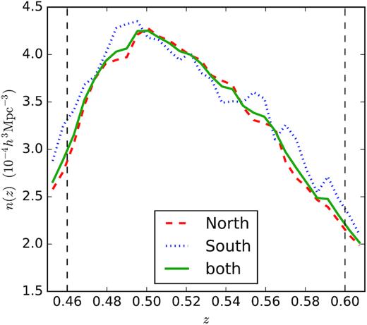
The CMASS DR12 galaxy comoving number density distribution across our redshift range. The red dashed line corresponds to the North Galactic Cap, whereas the blue dotted line corresponds to the South Galactic Cap. The green solid line shows the combined number density. The two vertical lines mark z = 0.46 and z = 0.6, respectively.
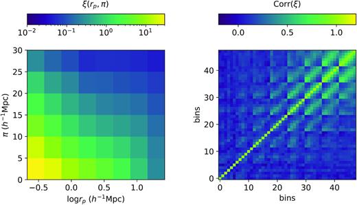
The redshift-space two-point correlation function (2PCF; left) of the BOSS CMASS DR12 galaxies at 0.46 < z < 0.6 and its corresponding covariance matrix (right). rp is the transverse comoving distance between galaxies. π is the LOS comoving distance between galaxies. The right-hand side shows the correlation matrix, calculated from 400 jackknife subsamples. The bins are formed by flattening the ξ bins column-by-column, with large bin number corresponding to large rp. For example, the bins 0–5 correspond to the first rp bin but increasing π.
We have corrected the fibre collision effect following the method of Guo et al. (2012), by separating galaxies into collided and decollided populations and assuming those collided galaxies with measured redshifts in the plate-overlap regions are representative of the overall collided population. The final corrected correlation function can be obtained by summing up the contributions from the two populations.
The correlation matrix is defined relative to the covariance matrix as |$\mathrm{Corr}(\xi)_{ij} = \mathrm{Cov}(\xi)_{ij}/\sqrt{\mathrm{Cov}(\xi)_{ii}\mathrm{Cov}(\xi)_{jj}}$|. The covariance matrix is calculated from 400 jackknife samples. The x and y axes of the right-hand panel in Fig. 2 show the same bins as on the left-hand panel, flattened in a column-by-column fashion such that the transverse separation rp increases with bin number. Overall, we see that the off-diagonal power is relatively small at small transverse scales and becomes more significant at larger transverse scales. This suggests that the error at small rp is shot-noise dominated, while sample variance becomes dominant at large rp.
3.2 N-body simulations and halo finders
For the primary results of this paper, we generate our galaxy mocks from the AbacusCosmos N-body simulation suite, generated by the fast and high-precision abacus N-body code (Garrison et al. 2016, 2018; Ferrer et al., in preparation; Metchnik & Pinto, in preparation).2 We use 20 boxes of comoving size 1100 h−1 Mpc with Planck 2015 cosmology (Planck Collaboration XIII 2016) at redshift z = 0.5. We quote the cosmology parameter values as Ωch2 = 0.1199, Ωbh2 = 0.02222, σ8 = 0.830, ns = 0.9652, h = 0.6726, and w0 = −1. These boxes are set to different initial phases to generate unique outputs. Each box contains 14403 dark matter particles of mass |$4\times 10^{10}\, h^{-1}\,\mathrm{ M}_{\odot }$|. The force softening length is 0.06 h−1 Mpc. Dark matter haloes are found and characterized using the rockstar (Behroozi et al. 2013) halo finder.
When testing the environmental assembly bias in Section 5.4, we also incorporate the AbacusSummit simulation suite, which is a set of large, high-accuracy cosmological N-body simulations designed to meet the cosmological simulation requirements of the Dark Energy Spectroscopic Instrument (DESI) survey (Levi et al. 2013). AbacusSummit consists of over 140 simulations most of which contain 69123 particles within a 2 h−1 Gpc volume, which yields a particle mass of 2.1 × 10⁹ h−1 M⊙.3
The AbacusSummit boxes that we employ include one with the primary Planck 2018 ΛCDM cosmology as the benchmark and four other boxes with perturbed cosmologies, specifically varying cosmological parameters Ωc and σ8. The Planck 2018 cosmology parameters are Ωch2 = 0.1200, Ωbh2 = 0.02237, σ8 = 0.811355, ns = 0.9649, h = 0.6736, w0 = −1, and wa = 0. Note that this is a slightly different cosmology than the Planck 2016 cosmology used for the AbacusCosmos simulations, the largest difference being a |$\sim \! 2{{\ \rm per\ cent}}$| smaller σ8 in the new cosmology. We concentrate our study of these simulations at redshift z = 0.5 and make use of the output data products including particle subsamples, CompaSO (Hadzhiyska et al., in preparation) and rockstar halo catalogues.
The two simulation suites also utilize different halo finders. The AbacusCosmos simulations use rockstar, whereas the AbacusSummit simulations use CompaSO.
rockstar is a temporal, phase-space halo finder considered to be highly accurate in determining particle–halo membership, as it uses information about both the phase-space distribution of the particles and their temporal evolution (Behroozi et al. 2013). This is because having information about the relative motion of two haloes makes the process of finding tidal remnants and determining halo boundaries substantially more effective, while having temporal information helps to maximize the consistency of halo properties across time, rather than just within a single snapshot.
The CompaSO halo-finding algorithm was designed for the AbacusSummit suite of high-performance cosmological N-body simulations, as a highly efficient on-the-fly group finder (Hadzhiyska et al., in preparation). CompaSO builds on the existing spherical overdensity (SO) algorithm by taking into consideration the tidal radius around a smaller halo before competitively assigning halo membership to the particles in an effort to more effectively deblend haloes. Among other features, the CompaSO finder also allows for the formation of new haloes on the outskirts of growing haloes, which alleviates a known issue of configuration-space halo finders of failing to identify haloes close to the centres of larger haloes.
A detailed comparison between the two halo finders will be made in Hadzhiyska et al. (in preparation).
4 METHODS
The fundamental technological challenge is to search a high-dimensional extended HOD parameter space for a prescription that best reproduces the observed redshift-space 2PCF signal and galaxy number density. Perhaps the most popular approach for fitting an extended HOD model on data is to employ a so-called emulator. The emulator approach is where we train a surrogate model of the observable within a HOD training set before we fit the best-fitting surrogate model on data. An example of an HOD emulator with the extended HOD model in this work was implemented in Yuan et al. (2020). However, we found that the emulator for such a high-dimensional parameter space has poor accuracy and breaks down outside the training range. The quadratic emulator model we employed was also not flexible enough for a wide training range to enable a comprehensive search. Thus, in this paper, we opt for a direct global optimization of the likelihood function to find the optimal HOD. A direct optimization has a much wider range in parameter space and is not limited by the shape of the surrogate model in an emulator. However, it requires repeatedly generating mock galaxy catalogues from simulations, which can be prohibitively expensive, especially since we are utilizing the particle catalogue in addition to the halo catalogue in this analysis.
In this section, we describe our likelihood function, its maximization, and then the key methods implemented to accelerate the HOD code.
4.1 The maximum likelihood routine
To minimize χ2, we utilize a global optimization algorithm known as covariance matrix adaptation evolution strategy (CMA-ES; Hansen & Ostermeier 2001). CMA-ES is an evolutionary algorithm that stochastically varies and selects on a school of candidate solutions, resembling the evolution of a biological system. In the simplest terms, the algorithm works by updating the mean and covariance matrix of the distribution to increase the probability of previously successful search vectors in each step until the candidate solutions converge to the global optimum. The algorithm also records and exploits the time-wise history of the search for faster stepping while also preventing premature convergence. The specific implementation of CMA-ES we use is part of the publicly available STOCHastic OPtimization for PYthon (StochOPy) package.4 To assess the error bars on the best fit, we run 22 Markov chain Monte Carlo (MCMC) chains initialized around the best fit with the emcee package (Foreman-Mackey et al. 2013). We quote our 1σ error bars as the standard deviation of the marginalized posterior distribution.
4.2 Accelerating the HOD code
The key challenge in our HOD global optimization is speed. Each HOD evaluation requires generating mock galaxies on the halo catalogues and then computing summary statistics. The first step is particularly time-consuming since we are using a particle-based HOD. In the following paragraphs, we describe several key speed-ups to enable a fast particle-based HOD implementation.
The first and most obvious speed-up comes from parallelization. Given that generating mock galaxies is a so-called ‘embarrassingly parallel’ problem on the halo level, the performance gain scales roughly linearly with the number of CPU cores utilized, given a sufficient amount of memory and I/O bandwidth. All computation in this analysis is done on a custom-built desktop, where we distribute the computation over 20 cores on a pair of Intel Xeon E5-2630v4 CPU clocked at 2.2 GHz for a roughly 20× performance gain.
Another ∼20× speed-up comes from utilizing a numba just-in-time (JIT) compiler (Lam, Pitrou & Seibert 2015), which converts slow python code to fast machine code. numba is especially powerful for long loops of unvectorized code, which is the case for generating mock satellite galaxies. Note that generating satellites is the main performance bottleneck as generating central galaxies does not query the particle subsamples. The numba compiler brings the time to generate the satellites down to ∼10× that of the centrals.
The third speed-up comes from pre-downsampling the haloes and particles for satellite generation. The idea here is that satellites are rare compared to centrals, especially at halo mass <1014. Thus, we aggressively downsample the haloes at smaller halo mass and correspondingly upweight the expected number of satellites in each of the downsampled haloes. This way, we significantly reduce the number of haloes looped over in each HOD evaluation without losing fidelity, yielding a significant performance improvement. Similarly, we can downsample the particles in the haloes to further increase performance. With our final choice of downsampling functions, we achieve another 3× speed-up in our HOD evaluation. We suspect that our downsampling is still relatively conservative, and an even greater speed-up is attainable.
I/O is another performance bottleneck. We largely overcome this by pre-loading the downsampled halo and particle file on memory before we start an optimization chain. To control memory usage, we only load relevant halo and particle information. Since the extended HOD parameters (s, sp, sv) only interact with the ranking of particle properties within each halo instead of the particle properties themselves, we can pre-compute these ranks and load them on memory. Another potential slowdown is when the HOD generates too many galaxies. To avoid this problem, we calculate the incompleteness factor fic to match the observed galaxy number density before we start an HOD evaluation. Then we scale down the number of centrals and satellites for each halo prior to assigning galaxies.
Finally, we compute the redshift-space 2PCF using the high-performance corrfunc code in parallel (Sinha & Garrison 2020). This specific computation turns out to be fast compared to generating mock galaxies. For the AbacusCosmos simulations, our final optimized pipeline, given our machine specifications, evaluates a new HOD over a ∼10 h−1 Gpc3 volume and computes its χ2 in roughly 7 s, 5 s of which are spent on generating mocks and 2 s on computing the 2PCF. The performance is similar for the AbacusSummit simulations. For the rest of this paper, we fit the HOD with only the first eight of the 20 AbacusCosmos simulation boxes, due to limitations in system memory. For the AbacusSummit fits, we only use one 2 h−1 Gpc box at each cosmology, which is equivalent to approximately six AbacusCosmos boxes in volume.
5 RESULTS
Table 1 summarizes the four key fits of this study. All four fits are constrained on the observed ξ(rp, π) and the observed galaxy number density. The four fits are identical except for which assembly terms are included. The first fit includes both A and Ae. The second and third fits only use one assembly bias term, A and Ae, respectively. The fourth fit includes neither. The comparison of these four fits lets us assess the importance of each assembly bias term. When a fit does not include an assembly bias parameter, we simply fix that parameter to 0. Besides the HOD parameters, we also list the best-fitting χ2, the degrees of freedom, the Bayesian information criterion (BIC), and the average halo mass per galaxy. The χ2 shown has been corrected for the finite simulation volume, and also corrected for the covariance matrix inversion bias following Hartlap, Simon & Schneider (2007). The limits of the top-hat prior constraints on the parameters are listed in the second column. The prior constraints on log M1 are not shown because we choose to constrain the satellite fraction 0 < fsat < 0.2 instead.
Summary of the key HOD fits in this study. The first column lists the HOD parameters, incompleteness factor fic, the final χ2, degrees of freedom, and the average halo mass per galaxy |$\log _{10}\bar{M}_\mathrm{ h}/\mathrm{ M}_\odot$|. The second column shows the prior constraints. The next four columns summarize the four key fits of this study. The prior constraints on log M1 are not listed because we choose to constrain the satellite fraction 0 < fsat < 0.2 instead. Note there is a one-to-one correspondence between M1 and fsat when the other HOD parameters are fixed. The corresponding best-fitting |$f_\mathrm{sat} = 9.4 \ {\rm per \ cent}$|. The errors shown are 1σ marginalized errors.
| Parameter name | Prior [min, max] | ξ fit with A and Ae | ξ fit with A | ξ fit with Ae | ξ fit with neither |
|---|---|---|---|---|---|
| log10(Mcut/h−1 M⊙) | [12.5, 14] | 13.33 ± 0.03 | 13.35 ± 0.03 | 13.37 ± 0.04 | 13.16 ± 0.02 |
| log10(M1/h−1 M⊙) | – | 14.47 ± 0.03 | 14.52 ± 0.02 | 14.33 ± 0.03 | 14.34 ± 0.02 |
| σ | [0.1, 2.0] | 0.61 ± 0.05 | 0.52 ± 0.07 | 0.94 ± 0.06 | 0.11 ± 0.09 |
| α | [0.7, 1.5] | 1.32 ± 0.05 | 1.39 ± 0.04 | 1.01 ± 0.04 | 1.16 ± 0.04 |
| κ | [0.1, 2.0] | 0.2 ± 0.1 | 0.1 ± 0.1 | 0.2 ± 0.1 | 0.2 ± 0.1 |
| s | [−1.0, 1.0] | 0.1 ± 0.1 | 0.0 ± 0.1 | 0.3 ± 0.1 | 0.6 ± 0.1 |
| sv | [−1.0, 1.0] | 0.8 ± 0.1 | 0.6 ± 0.1 | 0.1 ± 0.1 | 0.5 ± 0.1 |
| αc | [0.0, 2.0] | 0.22 ± 0.03 | 0.26 ± 0.01 | 0.07 ± 0.07 | 0.21 ± 0.02 |
| sp | [−1.0, 1.0] | −1.0 ± 0.1 | −0.9 ± 0.2 | −1.0 ± 0.1 | −1.0 ± 0.1 |
| A | [−1.0, 1.0] | −0.88 ± 0.08 | −0.79 ± 0.06 | – | – |
| Ae | [−1.0, 1.0] | 0.040 ± 0.009 | – | 0.032 ± 0.05 | – |
| fic | – | 0.91 | 1.00 | 0.74 | 0.67 |
| Final χ2 (degrees of freedom) | – | 50 (37) | 67 (38) | 73 (38) | 93 (39) |
| BIC | – | 92 | 107 | 111 | 128 |
| |$\log _{10}\bar{M}_\mathrm{ h}/\mathrm{ M}_\odot$| | – | 13.52 | 13.56 | 13.57 | 13.61 |
5.1 ξ(rp, π) fit with both A and Ae
The first (leftmost) HOD fit listed in Table 1 uses the full set of extended HOD parameters including both assembly bias terms. We achieve a good fit on ξ(rp, π), with a final χ2 = 50 (degrees of freedom = 37) and a BIC of 92. For comparison, if we fit the ξ(rp, π) with just the standard five-parameter HOD with no extensions, then we get χ2 = 151 and a BIC of 174. This shows that the standard five-parameter HOD is strongly disfavoured by the redshift-space correlation function.
Fig. 3 visualizes the corresponding best-fitting 2PCF. The left-hand panel shows the best-fitting projected 2PCF in orange and the observation in blue. The middle panel shows the normalized difference between the best-fitting ξ(rp, π) and the observation. The normalization σ(ξ) is derived from of the diagonal of the inverse covariance matrix, i.e. |$\sigma = 1/\sqrt{\mathrm{diag}(\boldsymbol{\sf C}^{-1})}$|. The right-hand panel shows the χ2 contribution from each bin, computed by multiplying array |$(\boldsymbol {\xi }_{\mathrm{mock}} - \boldsymbol {\xi }_{\mathrm{data}})$| with array |$\boldsymbol{\sf C}^{-1}(\boldsymbol {\xi }_{\mathrm{mock}} - \boldsymbol {\xi }_{\mathrm{data}})$| termwise. Summing over these terms gives the final |$\chi ^2_\xi$|, as in equation (11).
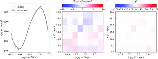
The best-fitting 2PCF using AbacusCosmos boxes, showing the ξ(rp, π) fit with both assembly bias terms A and Ae. The left-hand panel compares the projected 2PCF of the best-fitting HOD (orange) to that of the data (blue). The error bars on the data are computed from the diagonal of the inverted covariance matrix. The middle panel compares the best-fitting ξ(rp, π) with the data, where the errors, σ(ξ), are computed from the diagonal of the inverse covariance matrix. The right-hand panel showcases the contribution to the final χ2 from each bin.
We see that the best-fitting HOD does provide a good fit to the projected 2PCF and the redshift-space 2PCF. While a few bins in ξ(rp, π) seem to exhibit higher normalized error in the middle panel, it is important to note that the error bars σ(ξ) are computed from the diagonal of the inverse covariance matrix, underestimating the true uncertainty due to the high off-diagonal power in the covariance matrix (refer to the right-hand panel of Fig. 2). Thus, the actual difference between the mock and the data in these bins is less significant than it appears. The right-hand panel incorporates the full covariance matrix and is thus more informative in judging the consistency between data and mock in each bin. One bin (column 4 row 4) stands out as it contributes 7 to the final χ2. Excluding this bin from the HOD fit does not meaningfully change the final parameter values.
To take a closer look at the best-fitting parameter values, let us first take a look at the assembly bias parameters. The concentration-based assembly bias parameter A varies somewhat depending on the details of the fit, but generally yields rather negative best-fitting values from −0.5 to −0.9. The variation is likely affected by degeneracies within the HOD space and multimodality in the likelihood surface, in which case the error bar shown is underestimated. The negative A has the effect of moving galaxies into less massive and puffier haloes. In terms of its clustering signature, a negative A increases the projected clustering at intermediate and large transverse scales (rp > 1 h−1 Mpc) while reducing clustering at large LOS separations, especially at small transverse scales (rp < 1 h−1 Mpc), suggesting a smaller velocity dispersion. Lange et al. (2019) also show degeneracies between A and cosmology, specifically fσ8. Thus, a negative A could also indicate that our presumed fσ8 is too high. Unfortunately, we do not have a sufficiently large range in the cosmologies probed by our simulations to properly verify this possibility. Thus, we leave it as an opportunity for a future study.
The environment-based assembly bias parameter Ae yields a best-fitting value of 0.04 and is stable across different fits, suggesting that galaxies preferentially populate haloes in denser environments. We point out that the relative magnitudes of A and Ae parameters are deceptive as the actual amplitude of the effect depends on that value of the normalized concentration δc and the environment factor fenv (equation 5 and 7). The actual contribution of Ae = 0.04 and A = −0.8 on ξ(rp, π) are comparable in amplitude.
The other extended parameters also yield interesting fits. s, which sets the radial distribution of satellite galaxies, is slightly positive but consistent with zero. We find a large variation in the best-fitting sv, anywhere from 0.2 to 0.8, depending on the details of the fit. This variation is again likely due to degeneracies between sv and some other levers in the extended HOD, leading to multimodality in the likelihood surface. Regardless, the positive sv has the effect of increasing satellite velocities and thus increasing the Fingers-of-God effect. Unlike sv, the best-fit for the central velocity bias parameter αc is stable at ∼0.2 across different fits. This is consistent with the multipole fits in Guo et al. (2015). The best-fitting value of sp is also consistently close to −1 across our fits, suggesting that the observation strongly favours to put some satellites on highly eccentric orbits that pass through the central regions of the halo. sp is a novel addition to the HOD, and its significance possibly indicates the existence of a subset of infalling or splashback galaxies in the CMASS sample. This is an interesting result and we reserve a more detailed discussion on sp in a separate paper.
5.2 ξ(rp, π) fit without both A and Ae
The second and third fit in Table 1 only incorporate one assembly bias term, A and Ae, respectively. The fourth fit includes neither assembly bias terms. Compared to the first fit with both A and Ae, the second and third fit yield significantly worse χ2, with large increase to the BIC, ΔBIC = 15 and 19, respectively. Conversely, comparing to the fit with no assembly bias, the inclusion of either A or Ae leads to significantly better fits. Comparing the first fit and the fourth fit, we see that the inclusion of both assembly bias term is strongly favoured by the data, with a ΔBIC = −36. Thus, we conclude that the redshift-space 2PCF calls for the simultaneous inclusion of both a concentration-based assembly bias and an environmental assembly bias, at least in our HOD framework at Planck 2015 cosmology.
Fig. 4 shows the residuals in the redshift-space 2PCF ξ(rp, π) compared to the data when neither assembly biases is included in the fit, i.e. the last fit shown in Table 1. Compared to the middle panel of Fig. 3, where we show the residuals of the HOD fit including both assembly biases, we see that the residuals here are noticeably larger, especially at large rp ∼5–10 h−1 Mpc. The LOS structure reproduced by the no assembly bias fit is also worse, across all rp. To explain this, note that on the one hand, the concentration-based assembly bias A has a strong effect on the galaxy velocity dispersion as it moves galaxies into more or less massive haloes. Thus, A is strongly sensitive to the LOS structure of ξ(rp, π), at small and large rp. This explains why the inclusion of A improves the fit on the LOS structure of ξ(rp, π). The environmental assembly bias Ae, on the other hand, does not produce as strong a LOS signature, but it predominantly affects the projected clustering on intermediate scales rp ∼2–10 h−1 Mpc. This explains why the inclusion of Ae in the model reduces the residuals at rp ∼5–10 h−1 Mpc. This comparison between Fig. 4 and the middle panel of Fig. 3 directly showcases how the inclusion of the two assembly bias terms improve the ξ(rp, π) fit and highlights their importance in a flexible HOD model.
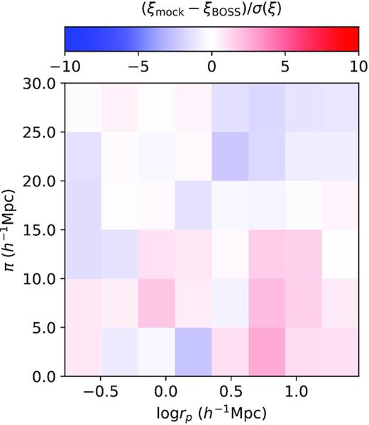
The residual in the redshift-space 2PCF ξ(rp, π) relative to the data when neither assembly biases is included in the HOD, corresponding to the last best fit listed in Table 1. Comparing to the fit including both assembly biases (middle panel of Fig. 3), we see significantly larger residuals at large rp, and worse prediction of the LOS structure.
In terms of the average halo mass per galaxy, we see that the inclusion of either assembly bias results in a 10–12 |${{\rm per\ cent}}$| decrease compared to the fit with no assembly bias, whereas the inclusion of both terms results in a |$23{{\ \rm per\ cent}}$| decrease. In comparison, a five-parameter HOD plus parameters s, A, and Ae constrained on the projected correlation function wp and galaxy number density gives an average mass of |$\bar{M}_\mathrm{ h} = 10^{13.62}\,\mathrm{ M}_\odot$|, |$26{{\ \rm per\ cent}}$| larger than that of the ξ(rp, π) fit with both assembly bias turned on. This indicates that the redshift-space 2PCF prefers to assign galaxies to lower mass haloes at fixed bias, and the two assembly bias terms give the HOD flexibility to do so, allowing for a much better fit. The projected 2PCF does not exhibit this preference, even when modelled with both assembly biases turned on. This result highlights the extra constraining power offered by the LOS structure of the redshift-space 2PCF. The decrease in typical halo mass for galaxies also has significant implications for the galaxy–galaxy lensing signal, as we will discuss in the following subsection.
While we should not overinterpret the final parameter values of these fits due to the poor χ2, we can still compare the parameter values across these fits to gain intuition on what exactly is driving the fit. When A is included, the fit prefers a strongly negative value, which has the effect of increasing large-scale clustering while decreasing the typical halo mass of galaxies. However, a negative A also results in a smaller velocity dispersion on the very small scale due to the less massive and puffier haloes. To compensate for this effect, the fit chooses a larger log10M1, α, and sv, which increases the Fingers-of-God effect on the small scale. In other words, it seems that the strong clustering amplitude at large scales is driving galaxies into less massive haloes with a negative A, and then the satellite distribution parameters are then tuned to match the small-scale Fingers-of-God signature.
The inclusion of Ae has a similar effect, where a positive Ae increases clustering on larger scales while decreasing the typical halo mass of galaxies. However, compared to A, the clustering signature of Ae is more dependent on rp, specifically its signature is strongest in the 1 < rp < 4 h−1 Mpc range and weakens beyond that, whereas the signature of A remains strong up to 30 h−1 Mpc. Ae also produces a weaker gradient along the LOS and has a rather small signature on the small scale (rp < 1 h−1 Mpc) compared to A. Thus, the inclusion of Ae triggers less of response from the parameters that control the satellites and the velocity dispersion, but it further decreases the average halo mass while boosting intermediate- to large-scale clustering.
5.3 The galaxy–galaxy lensing prediction
A well-known tension exists between galaxy clustering and galaxy–galaxy lensing. Leauthaud et al. (2017) found discrepancies of 20–40 |${{ \rm per\ cent}}$| between their measurements of galaxy–galaxy lensing for CMASS galaxies and a model predicted from mock galaxy catalogues generated at Planck cosmology that match the CMASS projected correlation function (Reid et al. 2014; Saito et al. 2016; see fig. 7 of Leauthaud et al. 2017). Lange et al. (2019) extended this result by finding a similar |${\sim } 25{{\ \rm per\ cent}}$| discrepancy between the projected clustering measurement and the galaxy–galaxy lensing measurement in the BOSS LOWZ sample. In Yuan et al. (2020), we reaffirmed this tension by fitting simultaneously the projected galaxy clustering and galaxy–galaxy lensing with an extended the HOD incorporating a concentration-based assembly bias prescription. The left-hand panel of Fig. 5 reproduces this tension, where the blue curve showcases the observed lensing signal of the CMASS sample, and the red curve shows the prediction of a HOD constrained on the projected 2PCF. The dashed green curve indicates the joint fit from Yuan et al. (2020). The best-fitting HOD corresponding to the red curve achieves a very good fit of the projected 2PCF (χ2 = 5.6 and degrees of freedom = 9), with |$\lt 1{{\ \rm per\ cent}}$| error across all bins. However, it provides a very poor lensing prediction, approximately 20–40 |${{ \rm per\ cent}}$| larger than the observation. The joint fit of the projected 2PCF wp and the galaxy–galaxy lensing shown in the dashed green curve fails to fit either observable well, resulting in a 10–20 |${{ \rm per\ cent}}$| discrepancy with the observed wp (shown in fig. 4 of Yuan et al. 2020) while reducing the lensing discrepancy by |${\sim }10{{\ \rm per\ cent}}$|, not enough to reconcile with the observation.
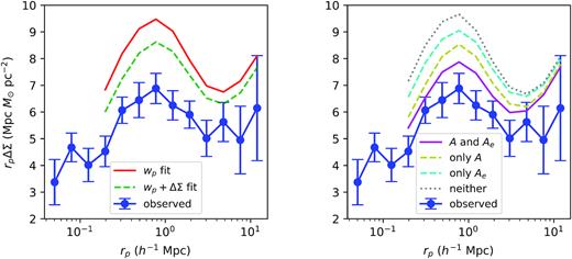
The comparison between the predicted galaxy–galaxy lensing signal and the observed galaxy–galaxy lensing signal. In both panels, the blue curve shows the observed lensing signal of the CMASS galaxy sample, quoted directly from Leauthaud et al. (2017). In the left-hand panel, the solid red curve shows the predicted lensing signal if we constrain the HOD with just the projected correlation function wp and the galaxy number density. The dashed green line shows the wp + ΔΣ emulator fit from Yuan et al. (2020). In the right-hand panel, the magenta curve shows the predicted lensing signal of our standard ξ(rp, π) fit, including both A and Ae. The dashed yellow (cyan) curve shows the prediction when we fit the ξ(rp, π) with only A (Ae). The grey dotted line shows the prediction when we do not include either assembly biases in the HOD model. We see that by fitting the full redshift-space correlation function and incorporating both assembly biases into the HOD, we significantly reduce the tension between data and predictions, down to about 1σ level.
The inclusion of both assembly bias terms (A and Ae) and switch to redshift-space 2PCF present an opportunity at reducing this tension. As we have shown, both assembly bias terms allow the redshift-space 2PCF to drive the fit in the direction of reducing the typical halo mass of galaxies. The right-hand panel of Fig. 5 shows the galaxy–galaxy lensing predictions of our redshift-space clustering fits. Again, the solid blue curve shows the measurement from Leauthaud et al. (2017) on the CMASS sample. The solid magenta line represents the ξ(rp, π) fit with both A and Ae, whereas the dashed yellow and cyan curves show the fit with just A and Ae, respectively. The dotted grey curve shows the fit with neither assembly bias terms. As expected, the introduction of both assembly bias terms leads to lower predicted lensing signal by assigning galaxies to less massive haloes.
The prediction of the ξ(rp, π) fit with both A and Ae matches the observation to within 1σ. This is a significant improvement compared to the 3σ discrepancies found with previous model predictions that fit the projected 2PCF wp using more simplistic HOD models (e.g. Reid et al. 2014; Rodríguez-Torres et al. 2016; Saito et al. 2016; Alam et al. 2017; Lange et al. 2019; Yuan et al. 2020). Comparing the predictions on the right-hand panel, we see that the decrease in the lensing signal really comes from a combination of incorporating assembly biases and constraining on the redshift-space 2PCF. Without the assembly bias terms, the ξ(rp, π) fit actually shows no improvement over the wp fit. The flexibility introduced by the assembly bias terms is what allows for a good ξ(rp, π) fit, which drives down the typical halo mass of galaxies, thus decreasing the lensing signal. Comparing the ‘with A’ fit on the right with the ‘wp + ΔΣ fit’ on the left, we see that the inclusion of just a concentration-based assembly bias results in a similar lensing prediction, even though one is constrained on ξ(rp, π) and the other is constrained on wp + ΔΣ. However, it is clear that the just a concentration-based assembly bias term is not sufficient in predicting the observed lensing signal. The combination of A and Ae is what uniquely brings the lensing prediction in agreement with the observation while also providing a good fit to ξ(rp, π).
It is interesting that the inclusion of A brings the galaxy–galaxy lensing prediction into better consistency with data than the inclusion of Ae. This hierarchy between A and Ae echoes with the fact that the inclusion of A yields a somewhat lower BIC and a slightly better fit to ξ(rp, π) than the inclusion of Ae in Table 1. This could mean that while both secondary dependencies are required to yield consistent predictions with data, the secondary dependency on concentration is more important than the dependency on environment in producing a more realistic HOD.
While we have shown that the combination of A and Ae is powerful in modelling both redshift-space clustering and galaxy–galaxy lensing, we do not claim that we have found the silver bullet to resolving the lensing tension. However, we believe that this represents a promising path towards reducing the lensing tension. A full solution of the lensing tension will likely also appeal to better handling of systematics and possibly small corrections in cosmology. We also do not claim that we have found the true prescription of galaxy assembly bias or the correct HOD model. Nevertheless, our findings highlight the importance of constructing flexible galaxy–halo connection models and employing more informative clustering statistics such as the redshift-space 2PCF. This result echoes the findings of Zu (2020), where the author found a sophisticated HOD model with detailed treatments of selection effects could reconcile the galaxy–galaxy lensing tension. However, it is argued that their model triggers an unrealistic satellite fraction (Lange et al. 2021). Amodeo et al. (2020) recently constrained cluster gas dynamics using Sunyaev–Zel'dovich effect and found an excess non-thermal pressure due to baryonic processes that would reduce the lensing tension by |$50{{\ \rm per\ cent}}$|. These energetic ejection processes towards larger halo radii are consistent with the positive environmental dependency that we found, highlighting the importance of baryonic structure beyond the typical virial radius of the halo.
5.4 Investigating the environmental assembly bias Ae
The novel environmental assembly bias parameter deserves some special attention as we showed that it behaves rather differently than the concentration-based assembly bias parameter and that it is indispensable in modelling the redshift-space 2PCF and predicting the observed lensing signal. We find further support for its legitimacy in the fact that its best-fitting value is remarkably stable across all our fits, despite variations to the HOD, likelihood function, compression of the data, and modest perturbations to the assumed cosmology. We visualize its best-fitting values across all these variations in Fig. 6, where the blue markers represent fits using the AbacusCosmos simulations, and the red markers represent fits using the AbacusSummit simulations. We briefly describe each of these fits as follows.
ξ(rp, π) fit. The ξ(rp, π) fit with both A and Ae as shown in Table 1, using eight AbacusCosmos boxes at Planck 2015 cosmology.
Seed 1–2. Same as ξ(rp, π) fit, except using different random number seeds to marginalize over shot noise effects.
Diff boxes. Same as ξ(rp, π) fit, except using a different set of eight of the 20 simulation boxes to marginalize over sample variance effects.
- Weak |$\chi ^2_{n_\mathrm{ g}}$|. Weakening the ng component of the likelihood function. Specifically, we modify |$\chi ^2_{n_\mathrm{ g}}$| as defined in equation (12) to essentially a step function:where σn ≈ 3 × 10⁻⁶ h3 Mpc−3 is the jackknife uncertainty on the observed ng. This new |$\chi ^2_{n_\mathrm{ g}}$| does not penalize the HOD for producing too many galaxies, allowing for rather low incompleteness factors. The best fit yields an incompleteness factor of fic = 0.67.(14)$$\begin{eqnarray*} \chi ^2_{n_\mathrm{ g}} = \left\lbrace \begin{array}{@{}l@{\quad }l@{}}\left(\frac{n_{\mathrm{mock}} - n_{\mathrm{data}}}{\sigma _{n}}\right)^2 & (n_{\mathrm{mock}} < n_{\mathrm{data}}), \\ 0 & (n_{\mathrm{mock}} \ge n_{\mathrm{data}}), \end{array}\right. \end{eqnarray*}$$
New π bins. Non-linear binning along the LOS direction to give more weight to the very small scales ∼1 h−1 Mpc. The new bins are π = [0, 0.5, 1, 5, 10, 20, 30].
Sigmoid ncent. Using a sigmoid function instead of an error function for |$\bar{n}_\mathrm{cent}$|. This test is done to address concerns that the error function was chosen arbitrarily for the HOD and might not correctly represent the physical central galaxy occupation distribution. The sigmoid function serves as an alternative ‘switch’ function from 0 to 1, providing a ‘softer’ ramp-up relative to the error function. Fig. 7 showcases the difference between a pair of similar sigmoid and error functions. We find that the best-fitting Ae is consistent with that of the error function fits. We also find no significant preference for using either the error function or the sigmoid function in the HOD.
wp + multipole. Fitting wp + ξ0 + ξ2 instead of ξ(rp, π). This fit and the next fit test whether different compressions of the redshift-space 2PCF affects the best-fitting Ae.
ξ(s, μ) fit. Fitting ξ(s, μ) instead of ξ(rp, π). s and μ essentially represent a polar coordinate system in the pair separation space, where s is the scalar separation between the two galaxies, and μ denotes the angle between the pair separation vector and the LOS.
Summit. ξ(rp, π) fit using one AbacusSummit box at Planck 2018 cosmology. The haloes are identified using the CompaSO halo finder instead of rockstar.
Summit + |$2{{\ \rm per\ cent}} \ \sigma _8$|. Same as Summit fit, but with |$2{{\ \rm per\ cent}}$| larger σ8 in the assumed cosmology.
Summit − |$2{{\ \rm per\ cent}} \ \sigma _8$|. Same as Summit fit, but with |$2{{\ \rm per\ cent}}$| lower σ8 in the assumed cosmology.
Summit + |$2{{\ \rm per\ cent}} \ \Omega _\mathrm{ M}$|. Same as Summit fit, but with |$2{{\ \rm per\ cent}}$| larger ΩM in the assumed cosmology.
Summit − |$2{{\ \rm per\ cent}} \ \Omega _\mathrm{ M}$|. Same as Summit fit, but with |$2{{\ \rm per\ cent}}$| lower ΩM in the assumed cosmology.
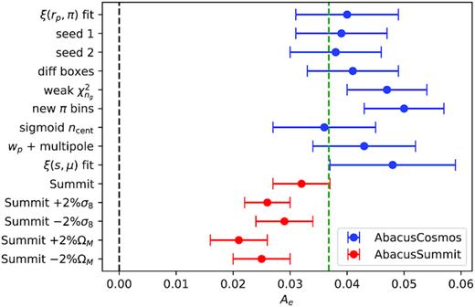
The best-fitting values of the environmental assembly bias parameter Ae across various fits. The blue markers represent fits using the AbacusCosmos simulations, whereas the red markers represent fits using the AbacusSummit simulations. The error bars are marginalized 1σ error bars. The dashed green line represents the average best-fitting value across all the fits.
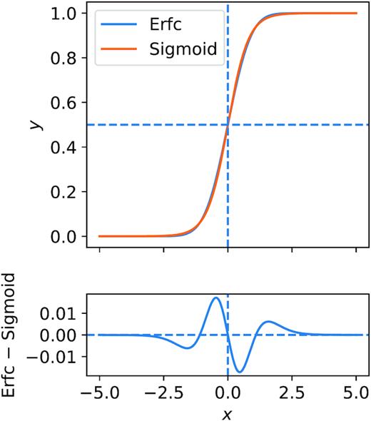
The top panel shows an example of a sigmoid function compared to a similar error function. The specific functions shown here are 0.5 erfc(x) in blue and sigmoid(2.5x) in orange. The bottom panel shows the difference between the two functions. Overall, the sigmoid produces a steeper incline in the middle but has a slower convergence to 1.
We see that within the AbacusCosmos fits in blue, all the Ae values are consistent within 1σ, regardless of all the variations we introduced. The Ae values for the AbacusSummit fits in red are more dispersed, likely caused by changes in cosmology and larger uncertainty due to the smaller simulation volume at perturbed cosmologies. The shift in Ae between the two sets of simulations is likely due to a combination of the slightly different cosmology (Planck 2015 versus Planck 2018), different N-body codes, and different halo finders (rockstar versus CompaSO). Regardless, the consistent 3σ–5σ preference for a positive Ae indicates that the environment dependence is a relatively standalone effect independent of concentration-based assembly bias and other HOD parameters, at least in our HOD framework. The positive Ae value with reasonable signal-to-noise ratio is also consistent with the environmental assembly bias signatures found in hydrodynamical simulations (Hadzhiyska et al. 2020, 2021; Xu et al. 2021). Finally, we note that while we find that the environmental dependence is important, we do not yet understand why it is so. We make a few attempts at gaining intuition on this phenomenon in Sections 6.3 and 6.4.
6 DISCUSSION
6.1 Testing HOD parameter recovery
To verify the effectiveness of our fitting procedure, we apply the fitting procedure to a mock redshift-space 2PCF generated from the simulations using a fiducial extended HOD. We also generate the jackknife covariance matrix from the same set of mocks, normalized to the BOSS CMASS volume. In the first test, we generate the mock observed 2PCF from the same set of eight simulation boxes that are then used to do the fitting. This avoids the effects of cosmic variance, and only tests whether our optimization routine is capable of recovering the correct underlying HOD. We find excellent recovery of all HOD parameters, with errors typically |$\lt 1{{\ \rm per\ cent}}$|. The parameter κ has the worst recovery, with errors of a few per cent.
In the second test, we generate the mock observed 2PCF from eight different simulation boxes than the ones used for fitting, thus introducing sample variance. We repeat this test for different fiducial HODs, we find excellent recovery of both A and Ae, with maximum recovery error significantly less than their 1σ error bars quoted in Table 1. We also generally get good recovery accuracy (<1σ error) on most other HOD parameters, such as Mcut, M1, σ, α, s, sv, αc, and sp. However, the recovery accuracy on κ is a notably worse, at around 2σ. This might be attributed to the fact that the redshift-space 2PCF is not particularly sensitive to changes to κ, as it only modifies satellite occupation at small halo mass. Overall, our tests show that at the current level of systematics, the two assembly bias parameters are well constrained by the redshift-space 2PCF on the scales that we chose. Most of the other extended HOD parameters are also well constrained relative to their error bars, except for κ.
6.2 Fitting the redshift-space multipoles
While in this work we adopted the novel approach of directly fitting the 2D ξ(rp, π), the more common approach is to fit the first multipoles of the redshift-space 2PCF. In principle, the full multipole expansion should contain the same information as the 2D ξ(rp, π). However, different choices in binning and the fact that most fits were done with only the first two or three multipole terms mean that different regions of the (rp, π) separation space enter the multipole fit with different weights. Thus, the first multipoles capture a different set of clustering information compared to ξ(rp, π).
The most relevant work is Guo et al. (2015), where the authors achieved a good fit on a set of BOSS CMASS redshift-space multipoles without invoking any assembly bias prescription in their HOD, seemingly contradicting our finding. Besides that fact that our study chooses a different data compression in ξ(rp, π), another key difference between Guo et al. (2015) and this study lies in our novel velocity bias model. While our velocity bias model changes the satellites’ velocities and positions simultaneously to preserve Newtonian physics, the Guo et al. (2015) model modifies the satellite velocities without changing their radial positions, allowing for exotic satellite trajectories that do not obey the physics of the potential well. It is possible that this extra flexibility in satellite velocity removes the need for assembly bias in the HOD model. To test this hypothesis, we perform ξ(rp, π) fits, replacing our velocity bias model with that of Guo et al. (2015). However, we continue to find strong evidence for assembly bias, where the inclusion of assembly bias parameter A improves the χ2/degrees of freedom by 1.
This suggests that the different data compression (ξ(rp, π) versus multipoles) might be responsible for the contradicting conclusions regarding assembly bias. To test this, we fit the first multipoles, up to l = 4, adopting the velocity bias model of Guo et al. (2015). Indeed, we find that, in this case, the inclusion of A improves the fit by a much smaller amount (Δχ2/degrees of freedom = 0.2), yielding weak evidence for assembly bias. Furthermore, we showcase the best-fitting multipoles in Fig. A1. We see that the best fit manages to reproduce the data up to l = 6, but fails to reproduce the data at l = 8. This suggests that perhaps the first multipoles do not capture the full redshift-space clustering information at these scales, and there is a significant amount of information leftover in the high multipoles. This might not be surprising considering the small-scale redshift-space distortion (RSD) signature is dominated by pairs with small transverse separation (rp ∼ 1 Mpc) and large LOS separation (π ∼ 20 Mpc). Such signature is poorly localized in a multipole decomposition. We also examine the multipoles of the ξ(rp, π) fit and find that while it does not reproduce the data at l = 2, 4 quite as well as the multipole fit, it does reproduce the data much better at l = 8. Thus, this shows that the multipoles capture a different subset of the full clustering information than ξ(rp, π), resulting in different HOD fits.
Saito et al. (2016) implement a subhalo abundance matching (SHAM) model based on the peak maximum circular velocity Vpeak to model the BOSS CMASS 2PCF. The Vpeak-based SHAM model is of particular interest here because it naturally accounts for some assembly bias as Vpeak is a derivative of the halo merger tree and thus encodes some assembly history information. However, while they found a good fit on the projected 2PCF, they found poor consistency with the first and second redshift-space multipoles. This again highlights how different compressions of the full redshift-space clustering capture different subset of the information content, and also the lack of constraining power of the projected 2PCF.
6.3 Alternative environment definitions and scale dependence
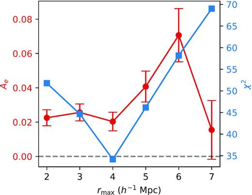
In this section, we further explore the environmental assembly bias by testing variations to the definition of halo environment. Specifically, we vary the radius, rmax, within which the local environment is calculated. Then, we test a different definition of the local environment altogether, where we use the Gaussian smoothed local density field instead of mass enveloped within rmax.
The left-hand panel of Fig. 8 shows the best-fitting environmental assembly bias parameter Ae and the corresponding best-fitting χ2 when we vary the maximum radius rmax of the halo environment definition. Note again that the environment is defined as the sum of the mass of neighbouring haloes beyond the virial radius but within rmax. We refer to this mass definition as the top-hat definition. We see that the amplitude of the Ae best-fitting peaks at rmax = 6 h−1 Mpc, whereas the smallest χ2 is achieved at rmax = 4 h−1 Mpc. At smaller and larger rmax, the best-fitting Ae trends towards zero and the χ2 increases. Qualitatively, this shows that the goodness-of-fit of the model is sensitive to the choice of rmax, specifically we find rmax ≈ 4–6 h−1 Mpc to be strongly preferred by the data.
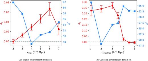
The scale dependence of the Ae fit. (a) The best-fitting environmental assembly bias parameter Ae and the corresponding best-fitting χ2 as a function of maximum radius of the environment rmax. (b) The same as (a), except the environment is now defined in terms of the local halo density field smoothed with a Gaussian of scale rsmoothed. The error bars represent 1σ uncertainties. We see that, in the top-hat case, a positive Ae is only preferred by the data when rmax ≈ 4–6 h−1 Mpc, and in the smoothed case, a positive Ae is only preferred when rsmoothed ≈ 2 h−1 Mpc.
The right-hand panel shows the best-fitting Ae and the corresponding χ2 for the Gaussian smoothed environment definition, where we define the environment as the local halo number density smoothed with a Gaussian kernel of scale rsmoothed. We see a qualitatively similar behaviour as the top-hat definition, where the goodness-of-fit of the model is strongly dependent on the choice of rsmoothed. In this case, we find rsmoothed ≈ 2 h−1 Mpc is the smoothing scale that best minimizes χ2 and maximizes the Ae value. This is qualitatively consistent with the preference for rmax ≈ 4–6 h−1 Mpc in the top-hat case, given the extended nature of a Gaussian filter. We should note that the actual value of Ae is not comparable between the two environment definitions, as the amplitude of Ae is degenerate with the amplitude of the environment parameter fenv (equation 7). Because the Gaussian smoothed environment is defined on the halo neighbour count while the top-hat environment is defined on mass, the amplitude and distribution of fenv are actually quite different between the two definitions.
Both panels suggest that the halo environment at some specific scale of a few megaparsecs is particularly informative of the assembly bias effects, at least for the particular observable we are fitting. While it is not clear what phenomena drive this preference for a specific scale, it does vote against explanations that focus on much smaller scales.
It is possible that the preference for specific rmax is a result of the scales that our redshift-space 2PCF is defined on, specifically from 0.169 to 30 h−1 Mpc in the transverse direction and from 0 to 30 h−1 Mpc in the LOS direction. As shown in fig. 4 of Xu et al. (2021), environment defined at different scales dramatically change its signature on galaxy clustering. Thus, it is possible that the same observable at a different scale would prefer environment defined within a different radius. To test this effect, we generate the redshift-space 2PCF at twice the scale, specifically in eight log-spaced bins from 0.338 to 60 h−1 Mpc in the transverse direction and six linearly spaced bins from 0 to 60 h−1 Mpc in the LOS direction. We fit this enlarged redshift-space 2PCF using our extended HOD with the top-hat environment definition and show the best-fitting values of Ae and the corresponding χ2 in Fig. 9. We see the same behaviour as the left-hand panel of Fig. 8 despite doubling the scales of the 2PCF, with the amplitude of Ae peaking at rmax = 6 h−1 Mpc and the χ2 minimized at rmax = 4 h−1 Mpc. This suggests that the scale preference in rmax is not a result of the scales imprinted in the 2PCF bins. We believe that this serves as further evidence that the local environment, specifically defined with an rmax = 4–6 h−1 Mpc, is a physically meaningful indicator of assembly bias and is likely tracing underlying processes happening at a few megaparsecs around haloes that truly drive the assembly bias signature.
The scale dependence of the Ae fit for the enlarged redshift-space 2PCF. The environment is defined with the top-hat, same as the left-hand panel of Fig. 8. The enlarged redshift-space 2PCF is computed in eight log-spaced bins from 0.338 to 60 h−1 Mpc in the transverse direction and six linearly spaced bins from 0 to 60 h−1 Mpc in the LOS direction. We see the same behaviour as the left-hand panel of Fig. 8, with the amplitude of the Ae best-fitting peaking at rmax = 6 h−1 Mpc and the χ2 minimized at rmax = 4 h−1 Mpc.
It is beyond the scope of this paper to explore the exact underlying processes that drive the environmental assembly bias signature, but we speculate that galaxies and haloes in dense environments undergo processes such as mergers, tidal disruptions, and feedback processes, whereas galaxies in underdense environments evolve mostly passively. These processes can lead to environment dependence in halo occupation. Amodeo et al. (2020) found observational evidence of baryons being expelled beyond the halo virial radius due to a number of feedback effects. The same study also found that this effect could account for up to 50 |${{ \rm per\ cent}}$| of the lensing tension. Another likely relevant phenomenon is the splashback radius (Adhikari, Dalal & Chamberlain 2014; Diemer & Kravtsov 2014; More et al. 2015), where studies have found that a traditional halo boundary definition such as rvirial excludes some gravitationally bound subhaloes on highly eccentric orbits. Other parallel studies have also suggested that a more physical halo radius is ∼2–3 times larger than the traditional virial radius (Wetzel et al. 2014; Wetzel & Nagai 2015; Sunayama et al. 2016). In the context of HOD models, it might be better to consider these splashback haloes as part of the host halo instead of as individual haloes in the vicinity of larger haloes. The fact that we get an extreme best-fitting value for sp, which puts some satellites on highly eccentric orbits, might further be indicative of splashback haloes. It is possible that the incorporation of splashback radius could alleviate the need for the environmental assembly bias. In fact, Mansfield & Kravtsov (2020) found that the splashback radius can account for much, though not all, of the halo assembly bias signature in simulations.
The importance of halo environment and the recent pushes to enlarge halo boundaries might also point to shortcomings of the halo model overall. In the context of galaxy–halo connection models, instead of populating galaxies per halo, we might get closer to the true galaxy distribution by populating galaxies in larger groups, which are loosely defined as a group of closely associated haloes and their local environment. Such a group-based galaxy occupation model, if correctly defined, could eliminate the need to account for local environment and to redefine halo radii. It can significantly simplify existing extended HOD models, such as the one we used in this paper. We defer an exploration of this topic to a future paper.
6.4 Comparisons to previous studies on environment-based HOD
Two previous papers, Hadzhiyska et al. (2020) and Xu et al. (2021), systematically tested the effectiveness of various secondary HOD dependences in capturing the assembly bias signature, Hadzhiyska et al. (2020) through hydrodynamical simulations and Xu et al. (2021) through semi-analytical models. While they both found the halo environment to be an excellent indicator of assembly bias, there are some key differences between our work and the two previous papers.
In terms of galaxy samples, in this work we are focusing on LRGs, whereas both previous works focused on much less massive L⋆-type galaxies. Hadzhiyska et al. (2020) considered a mass-selected sample of L⋆-type galaxies with a number density of 1.3 × 10⁻³ h3 Mpc−3, an order of magnitude higher than our LRG sample. Xu et al. (2021) similarly looked at three samples of mass-selected L⋆-type galaxies of density n1 = 0.00316 h3 Mpc−3, n2 = 0.01 h3 Mpc−3, and n3 = 0.0316 h3 Mpc−3, which correspond to stellar mass thresholds of 3.88 × 10¹⁰, 1.42 × 10¹⁰, and 0.185 × 10¹⁰ h−1 M⊙, respectively. In comparison, CMASS LRGs are believed to have a typical stellar mass of a few times 1011 M⊙ (Maraston et al. 2013).
The definition of halo environment is also different across all three works. Our work largely inherits the environment definition from Hadzhiyska et al. (2020) with minor differences, namely the normalized enclosed mass of subhaloes within 5 h−1 Mpc. Most notably, Hadzhiyska et al. (2020) picked the r200m as the inner radius of the environment, while we used the virial radius for convenience. Xu et al. (2021), however, defined their halo environment as the local mass overdensity smoothed with a Gaussian filter, computed with all simulation particles instead of just subhaloes. They found that the smoothed overdensity with a filter scale of 1.25 h−1 Mpc best predicts the assembly bias signature. In a more recent work, Hadzhiyska et al. (2021) adopt an environment definition more similar to that of Xu et al. (2021), which uses the smoothed matter density field (with a Gaussian kernel of scale 1.1 Mpc h−1) around a halo to quantify its environment dependence. They show that augmenting the HOD model with a secondary dependence on environment in a manner that matches the two-point clustering, also successfully recovers additional statistical probes of the galaxy distribution such as the galaxy–galaxy lensing signal, the void–galaxy cross-correlation function, and moments of the galaxy density field. In this work, we find a somewhat larger optimal radius, which can be attributed to the different environment definitions and the different galaxy samples. It is also possible that different underlying physical processes drive the environmental assembly bias in L-type galaxies versus in LRGs. Finally, we caution that all these studies are limited by the fidelity of the hydrodynamical simulations and the semi-analytical models used.
7 CONCLUSION
In this paper, we model the observed redshift-space 2PCF of BOSS CMASS galaxy sample with an extended HOD model that includes two prescriptions of galaxy assembly bias and other physically motivated additions. We found that while the standard five-parameter HOD provides a poor fit to the redshift-space 2PCF (χ2 = 151, d.o.f = 42), the extended HOD achieves a substantially better fit with χ2 = 50 (d.o.f = 37; see Table 1 and Fig. 3). The redshift-space 2PCF also strongly prefers the simultaneous inclusion of both A and Ae, which, respectively, represent the assembly bias associated with halo concentration and halo environment. The preference for HOD models incorporating A and Ae is expressed with their corresponding ΔBIC: ΔBIC = 19 for A and ΔBIC = 15 for Ae. The HOD model that includes both assembly biases is strongly favoured over an HOD that includes neither, with ΔBIC = 36. When only one assembly bias term is included, the fit on the redshift-space 2PCF is significantly worse than when both assembly bias terms are included. Our results highlight the importance of a flexible assembly bias and HOD model in accurately modelling redshift-space clustering on the non-linear scale and expose the deficiencies of the standard five-parameter HOD model in producing realistic galaxy distributions.
The best fit yields a negative concentration-based assembly bias parameter A (∼10σ, preferentially assigning galaxies to puffier less massive haloes) and a positive environmental assembly bias parameter Ae (∼3σ–5σ, preferentially assigning galaxies to less massive haloes in denser environments). Compared to the projected correlation function, the redshift-space 2PCF pushes both assembly bias parameters in the direction of reducing typical halo mass per galaxy at fixed clustering, showcasing the extra constraining power contained in the LOS structure of the redshift-space 2PCF. Specifically, the inclusion of A decrease the average halo mass per galaxy by |$12{{\ \rm per\ cent}}$|, whereas the inclusion of Ae decreases the average halo mass by |$10{{\ \rm per\ cent}}$|. The HOD fit with both assembly biases constrained on redshift-space 2PCF yields |$26{{\ \rm per\ cent}}$| lower average halo mass compared to an HOD constrained on the projected correlation function.
We additionally showed that, by assigning galaxies to lower mass haloes, the extended HOD constrained on the redshift-space 2PCF predicts the observed galaxy–galaxy lensing signal to within 1σ (Fig. 5). This represents a significant improvement compared to predictions by HODs constrained on the projected 2PCF. This result translates the perceived tension between galaxy clustering and lensing to a tension between more informative clustering measurements and oversimplified galaxy–halo connection models. This result again highlights the importance of building more flexible galaxy–halo connection models and utilizing the more informative statistics such as the redshift-space 2PCF.
We offer strong evidence for including an environmental galaxy assembly bias term in the HOD. In addition to showing how the environmental assembly bias significantly improves the redshift-space 2PCF fit and the lensing prediction, we further showcase the consistency of a positive Ae fit over variations to the fitting routine, variations to the HOD model, and modest perturbations to the cosmology (Fig. 6). Combining this result with previous simulation studies that showed halo environment as an excellent indicator of assembly bias and being able to recover various observables, we believe an environmental assembly bias term is a physical and indispensable addition to the HOD. We recommend that future studies include environmental assembly bias in their HOD prescriptions in order to construct more realistic galaxy mocks.
In order to better understand the underlying processes driving the environmental dependence, we tested different maximum radii in the environment definitions, and we found that halo environment defined on scales of around 4–6 h−1 Mpc is preferred by the data (Fig. 8). This scale preference holds even when doubling the bin sizes of the observed 2PCF (Fig. 9). This suggests that the preference for 4–6 h−1 Mpc is not a result of the specific scales chosen when binning the observable, but rather determined by the underlying physical processes that exhibit a similar characteristic scale. We speculate that such processes are intrahalo and might include mergers, tidal disruptions, and feedback processes. We also suggest that the dependence on environment within 4–6 h−1 Mpc might also point to the need to define haloes at a much larger radius, such as the splashback radius.
While we found strong observational evidence for our prescriptions of assembly bias, there is no guarantee that our prescriptions capture the full underlying galaxy assembly bias effect. It is entirely possible that a better and possibly more simplistic assembly bias prescription can achieve the same or even better fit on the redshift-space galaxy clustering and galaxy–galaxy lensing. In upcoming papers, we plan on continuing to explore more physically motivated halo properties as sources of assembly bias, potentially leveraging the halo merger tree and constructing mass-dependent assembly bias prescriptions. We additionally plan on performing a joint analysis on the redshift-space 3PCF, galaxy–galaxy lensing, and the squeezed three-point correlation function (Yuan, Eisenstein & Garrison 2017) with our extended HOD model to derive cosmological constraints.
ACKNOWLEDGEMENTS
We would like to thank Lehman Garrison, Johannes Lange, Jeremy Tinker, Joe DeRose, Andrew Hearin, Martin White, Andrew Zentner, and Josh Speagle for fruitful discussions. DJE is supported by U.S. Department of Energy grant DE-SC0013718 and as a Simons Foundation Investigator. SB is supported by Harvard University through the ITC Fellowship. HG is supported by the National Science Foundation of China (Nos 11773049, 11833005, 11828302, and 11922305).
DATA AVAILABILITY
The simulation data are available at https://lgarrison.github.io/AbacusCosmos/ and https://abacussummit.readthedocs.io/en/latest/. Researchers wishing to gain access to the extended HOD code can refer to the publicly available grand-hod code at https://github.com/SandyYuan/GRAND-HOD or contact the lead author of this paper for details.
Footnotes
For more details, see https://lgarrison.github.io/AbacusCosmos.
For more details, see https://abacussummit.readthedocs.io/en/latest/abacussummit.html.
REFERENCES
APPENDIX: MULTIPOLE FITS
In Section 6.2, we performed a fit on the redshift-space multipoles, adopting the velocity bias model of Guo et al. (2015). The resulting best-fitting multipoles and projected correlation function wp are shown in Fig. A1. We see that the multipole fit reproduces the data well up to l = 6, but is inconsistent with the data at l = 8. This suggests that the first three multipoles fail to capture the full information of redshift-space clustering and there is significant amount of information leftover in the higher multipoles.
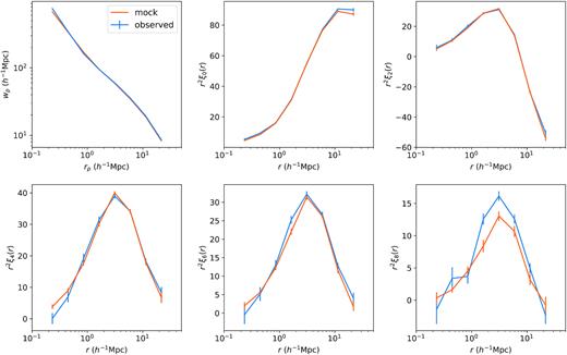
The redshift-space multipole fit up to l = 4. The fit reproduces the data well up to l = 6, but fails to reproduce the data at l = 8. This suggests that there is significant information leftover in the higher order multipoles.
