


ABSTRACT
The detonation of a helium shell on top of a carbon–oxygen white dwarf has been argued as a potential explosion mechanism for Type Ia supernovae (SNe Ia). The ash produced during helium shell burning can lead to light curves and spectra that are inconsistent with normal SNe Ia, but may be viable for some objects showing a light-curve bump within the days following explosion. We present a series of radiative transfer models designed to mimic predictions from double-detonation explosion models. We consider a range of core and shell masses, and systematically explore multiple post-explosion compositions for the helium shell. We find that a variety of luminosities and time-scales for early light-curve bumps result from those models with shells containing 56Ni, 52Fe, or 48Cr. Comparing our models to SNe Ia with light-curve bumps, we find that these models can reproduce the shapes of almost all of the bumps observed, but only those objects with red colours around maximum light (B − V ≳ 1) are well matched throughout their evolution. Consistent with previous works, we also show that those models in which the shell does not contain iron-group elements provide good agreement with normal SNe Ia of different luminosities from shortly after explosion up to maximum light. While our models do not amount to positive evidence in favour of the double-detonation scenario, we show that provided the helium shell ash does not contain iron-group elements, it may be viable for a wide range of normal SNe Ia.
1 INTRODUCTION
One of the most debated aspects of research on Type Ia supernovae (SNe Ia) is whether multiple progenitor systems are needed to explain the entire population (see Livio & Mazzali 2018; Wang 2018; Jha, Maguire & Sullivan 2019; Soker 2019, for recent reviews of SNe Ia). Despite significant work throughout the years, the question remains whether SNe Ia primarily result from Chandrasekhar- or sub-Chandrasekhar-mass white dwarfs.
To trigger the detonation of a sub-Chandrasekhar-mass white dwarf, early models invoked scenarios in which a massive helium shell (≲0.2 M⊙) accumulates on the surface of the white dwarf (e.g. Livne 1990; Livne & Glasner 1991; Woosley & Weaver 1994). As the mass of the helium shell increases through accretion, the density and temperature at the base of the shell also increase. Eventually convective nuclear burning may develop and potentially transition to a detonation. Following ignition of the shell, a secondary detonation may be triggered in the core. This secondary detonation can be triggered in multiple ways (converging shock, edge-lit, or scissors mechanism; Livne 1990; Livne & Glasner 1991; Moll & Woosley 2013; Gronow et al. 2020); however, the end result is the same – complete disruption of the white dwarf. This is the so-called double-detonation scenario. Within these models, most studies find that burning in the helium shell proceeds mostly to nuclear statistical equilibrium (NSE) – producing a large amount of 56Ni and other iron-group elements (IGEs). Such a large mass of IGEs in the outer ejecta leads to significant line blanketing that generally does not agree with observations of SNe Ia (Hoeflich & Khokhlov 1996; Nugent et al. 1997).
Given the adverse impact of the helium shell ash on the light curves and spectra, there has been significant interest in minimizing its effects. Neglecting any helium shell altogether, models invoking pure detonations of isolated, bare sub-Chandrasekhar-mass white dwarfs have been shown to broadly reproduce the light curves and spectra of normal SNe Ia (Sim et al. 2010b; Goldstein & Kasen 2018; Shen et al. 2018). Such white dwarfs, however, will not spontaneously detonate and therefore these explosions do not occur naturally. Alternatively, models with thin helium shells may also be a viable pathway to explain normal SNe Ia. Bildsten et al. (2007) showed that ignition within the helium shell can be achieved for much lower masses of ∼0.02 M⊙, but they did not consider the possibility of core ignition following the initial helium shell detonation. Subsequent core ignition was shown to be robustly achieved by Fink, Hillebrandt & Röpke (2007), Fink et al. (2010), and Shen & Bildsten (2014) for high-mass white dwarfs (≳0.8 M⊙). In spite of these lower shell masses, models presented by Kromer et al. (2010) and Gronow et al. (2020) remain inconsistent with the observed light curves and spectra of normal SNe Ia. Recently, Polin, Nugent & Kasen (2019) presented a suite of double-detonation models covering a range of core and shell masses (from 0.6 to 1.2 M⊙ and 0.01 to 0.1 M⊙, respectively) and find that some models with thin helium shells do produce spectra that resemble normal SNe Ia.
In addition to producing strong line blanketing, the presence of IGEs in the helium shell ash has an important consequence for the light curves predicted by double-detonation explosions. Noebauer et al. (2017) and Jiang et al. (2017) have shown that the production of short-lived radioactive isotopes (56Ni, 52Fe, and 48Cr) in the shell results in a distinct bump in the early light curve (within approximately 3 d of explosion). Studies of samples of SNe Ia (e.g. Bianco et al. 2011; Olling et al. 2015; Papadogiannakis et al. 2019; Miller et al. 2020b) have shown that the evidence for clear bumps is relatively rare, but a few candidate objects have been proposed (e.g. Hosseinzadeh et al. 2017; Jiang et al. 2017; De et al. 2019; Li et al. 2019; Miller et al. 2020a).
Qualitatively similar bumps in the early light curves of SNe Ia are also suggested to be produced via different mechanisms, such as the presence of a 56Ni excess in the outer ejecta (Magee & Maguire 2020), interaction with a companion star (Kasen 2010), or interaction with circumstellar material (CSM; Piro & Morozova 2016). An excess of 56Ni in the outer ejecta may result from plumes of burned ash rising to the surface of the white dwarf during explosion. As the 56Ni decays to 56Co, the radiation produced is able to quickly escape from the ejecta surface and results in a light-curve bump. The luminosity and duration of the bump depend on both the mass and distribution of 56Ni. In the interaction scenarios, a light-curve bump may be produced due to cooling of the shocked ejecta following the interaction. For companion interaction, the bump is affected by the nature of the companion, with more evolved stars producing stronger interaction signatures. In both cases, the mass and extent of the interacting material will also determine the luminosity and duration of the bump.
Maeda et al. (2018) specifically investigate the different early light-curve signatures predicted by the double-detonation scenario and interaction. The models presented by Maeda et al. (2018) show significant overlap between these two scenarios, in terms of the duration and luminosity of the bump, but the double detonation in general produces somewhat redder colours. Maeda et al. (2018) show that this is at least partially due to the specific IGEs present in the shell.
Aside from the mass of the helium shell, it has also been suggested that its composition can play an important role during nuclear burning, and can dramatically affect the post-explosion observable properties. Kromer et al. (2010) presented a model in which the helium shell was polluted by carbon (34 per cent by mass) and found that burning within the shell did not proceed to NSE, but instead stalled earlier in the α-chain. In this case, the lack of IGE in the shell produced light curves and spectra that are generally consistent with normal SNe Ia. In addition, Townsley et al. (2019) recently showed that the inclusion of other isotopes, besides carbon, can also dramatically affect the post-explosion composition of the shell and produce observables comparable to normal SNe Ia. Therefore, there is considerable scope for variation in the burning products produced in the shell.
In this work, we present radiative transfer simulations exploring a range of ejecta models that are designed to parametrize and broadly mimic predictions from double-detonation explosion models. We perform the first large-scale exploration of various compositions for the helium shell following explosion, and determine the range of models that do and do not reproduce observations of SNe Ia. Although different helium shell compositions in parametrized models were previously studied by Maeda et al. (2018), here we explore a wider range of compositions in the helium shell, as well as multiple shell masses for a given core mass. In Section 2, we discuss the radiative transfer code turtls used in this work (Magee et al. 2018). Section 3 presents our approach to constructing parametrized double-detonation models. In Section 4, we discuss the impact of the helium shell composition on the model observables, while in Section 5 we show the impact of the mass of burned material above the core. The rise times and early light-curve bumps of our models are discussed in Section 6. In Section 7, we compare to existing models with varying 56Ni distributions. Comparisons to observations of normal SNe Ia are presented in Section 8, while in Section 9 we compare to SNe Ia showing a bump in the early light curve. For all spectral comparisons, spectra have been corrected for Milky Way and host extinction, where appropriate, and were obtained from WISeREP (Yaron & Gal-Yam 2012). Finally, we present our conclusions in Section 10.
2 RADIATIVE TRANSFER MODELLING
We use the one-dimensional radiative transfer code turtls (Magee et al. 2018) to perform our simulations. All model light curves and spectra presented in this work are freely available on GitHub1. turtls is described in detail by Magee et al. (2018). Here, we provide a brief overview of the code and outline changes implemented for this study.
turtls is a Monte Carlo radiative transfer code following the methods of Lucy (2005) (see Noebauer & Sim 2019, and references therein, for a review of Monte Carlo radiative transfer methods). turtls is designed for modelling the early time evolution of thermonuclear SNe. For each simulation, the density and composition of the model ejecta are defined in a series of discrete cells. Monte Carlo packets representing bundles of photons are injected into the model region, tracing the decay of radioactive isotopes. We have updated turtls to account for energy generated by the 52Fe → 52Mn |$\rightarrow$|52Cr and 48Cr |$\rightarrow$|48V → 48Ti decay chains, which can contribute significantly to the luminosity and overall evolution of the model in the double-detonation scenario (Noebauer et al. 2017). Isotope lifetimes and decay energies are taken from Dessart et al. (2014).
For all simulations presented in this work, we use a start time of 0.5 d after explosion. In Appendix A, we show the results of some of our convergence tests with earlier start times. These tests demonstrate that, despite the short half-lives of many of the included isotopes, a start time of 0.5 d after explosion does not significantly alter the synthetic observables and does not impact our conclusions. Once packets are injected into the model region, their propagation is followed until either they escape or the simulation ends. Due to the assumption of local thermodynamic equilibrium (LTE) within turtls, simulations are stopped at 30 d after explosion. We also note that as a consequence of this assumption, our models do not predict the presence of helium features, despite the potential for a large amount of unburned helium. Previous studies have shown that a non-LTE treatment of helium is required to produce spectral features for the conditions typical of SN ejecta (Hachinger et al. 2012; Dessart & Hillier 2015; Boyle et al. 2017). At the start of each simulation, packets are injected as γ-packets (representing γ-ray photons) and treated with a grey opacity of 0.03 cm2 g−1. Following an interaction with the model ejecta, γ-packets are converted to optical radiation packets (r-packets). For these packets, we use tardis (Kerzendorf & Sim 2014; Kerzendorf et al. 2018) to calculate the non-grey expansion opacities and electron-scattering opacities within each cell during the current time-step. During each time-step, we extract a ‘virtual’ spectrum using the so-called event-based technique (e.g. Long & Knigge 2002; Sim et al. 2010a; Kerzendorf & Sim 2014; Bulla, Sim & Kromer 2015; Magee & Maguire 2020). Light curves are calculated via the convolution of synthetic virtual spectra with the desired set of filter functions at each time-step.
In Fig. 1, we show a comparison of our model light curves including the new decay chains to those calculated by Noebauer et al. (2017), using the radiative transfer code stella (Blinnikov et al. 1998, 2006) for the same model structure. This model involves the detonation of a 0.055 M⊙ helium shell on a 1.025 M⊙ carbon–oxygen white dwarf. The resulting explosion leads to the production of 0.55 M⊙ of 56Ni in the white dwarf core. The helium shell ash following explosion is dominated by IGEs, which includes ∼0.002 M⊙ of 56Ni, 0.006 M⊙ of 52Fe, and 0.004 M⊙ of 48Cr. Fig. 1 verifies that with our implementation of the additional decay chains, turtls can broadly match the light curves of Noebauer et al. (2017). The early light-curve bump observed in our models is somewhat less pronounced than that in the Noebauer et al. (2017) model, which is likely a result of differences in the treatment of opacities, for example.
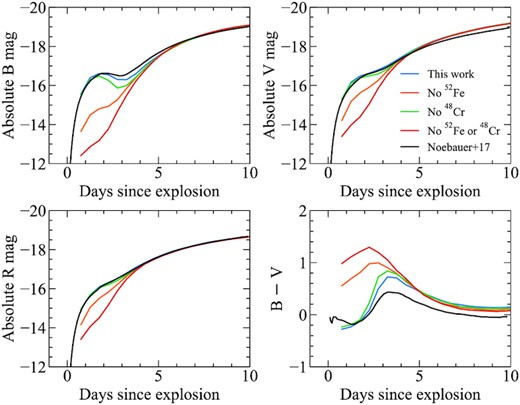
Comparison between the sub-Chandrasekhar-mass double-detonation model calculated by Noebauer et al. (2017) using stella (black) and our calculation using turtls (blue).
We also show light curves in Fig. 1 calculated including the 52Fe → 52Mn |$\rightarrow$|52Cr chain, the 48Cr → 48V |$\rightarrow$|48Ti chain, or neither, as a further demonstration of their contribution to the early luminosity. We note that in all cases, the 56Ni |$\rightarrow$|56Co |$\rightarrow$|56Fe decay chain is included. Including these additional chains produces an ∼4 mag increase in the brightness by approximately 2 d after explosion. Fig. 1 shows that despite the short half-lives of both the parent and daughter isotopes (t1/2 = 0.345 and 0.015 d, respectively), the 52Fe |$\rightarrow$|52Mn |$\rightarrow$|52Cr chain contributes significantly to the early luminosity within the first few days of explosion. For this model, the early bump reaches a peak B-band magnitude of −16.7 mag approximately 1.8 d after explosion. At this time, the instantaneous energy deposition rate from material in the shell reaches ∼1.3 × 1042 erg s−1 and dominates the luminosity output of the model, which is consistent with expectations from Arnett’s law (Arnett 1982).
3 CONSTRUCTING THE DOUBLE-DETONATION MODEL SET
In the following section, we discuss our approach to creating a parametrized description of the ejecta in double-detonation explosions. Our strategy is based on capturing and exploring the variation present across a range of published models in a systematic way. Each of our models is controlled by the following parameters: the mass of the carbon–oxygen core, the mass of the helium shell, the fraction of the helium shell burned during the explosion, and the dominant α-chain product produced in the shell burning. The range of input parameters used is shown in Table 1. The name of each model is also derived based on these parameters; for example, WD1.00_He0.04_BF0.50_DP56Ni refers to a model with a core mass of 1.0 M⊙ and a helium shell mass of 0.04 M⊙, of which 50 per cent is burned, and the dominant product produced in the shell is 56Ni. The range of parameters explored was chosen to broadly cover and bracket the values predicted by various explosion models, but we stress that they are not exact reproductions of existing models.
Ejecta model parameters.
| Core mass | Helium shell | Fraction of | Dominant burning |
|---|---|---|---|
| mass | shell burned | product in shell | |
| M⊙ | M⊙ | ||
| 0.90 | 0.01, 0.04, 0.07, 0.10 | 0.20, 0.50, 0.80 | 32S–56Ni |
| 1.00 | 0.01, 0.04, 0.07, 0.10 | 0.20, 0.50, 0.80 | 32S–56Ni |
| 1.10 | 0.01, 0.04, 0.07, 0.10 | 0.20, 0.50, 0.80 | 32S–56Ni |
| 1.20 | 0.01, 0.04, 0.07, 0.10 | 0.20, 0.50, 0.80 | 32S–56Ni |
For each model, we require a density profile for the ejecta. The density profiles presented in Magee et al. (2018, 2020) were designed to broadly mimic those from a variety of explosion scenarios. In particular, the exponential density profile with a kinetic energy of 1.4 × 1051 erg from Magee et al. (2020) bears a striking similarity to the models of Kromer et al. (2010) and Polin et al. (2019), although the density in the outer ejecta is slightly higher. We therefore take this model as our nominal profile shape and simply scale the density to the appropriate ejecta mass, which is given by the sum of the core and helium shell masses. A demonstrative comparison between model 3 of Kromer et al. (2010) and two of our models is shown in Fig. 2(a). We note that the core mass of model 3 (1.025 M⊙) is slightly higher than that of these models (1.0 M⊙), and we show two shell masses (0.04 and 0.07 M⊙) to bracket the 0.055 M⊙ shell of model 3.
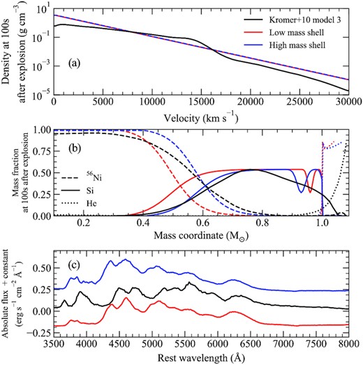
Comparison of properties for Kromer et al. (2010) model 3 (1.025 M⊙ core, 0.055 M⊙ helium shell) and our models with a 1.0 M⊙ core and 0.04 M⊙ (red) and 0.07 M⊙ (blue) helium shell. Panel a: Comparison between model density profiles. Panel b: Comparison between model compositions. Panel c: Maximum light spectra for all models (see Section 3 for further details). Spectra are offset vertically for clarity.
3.1 Composition of the core
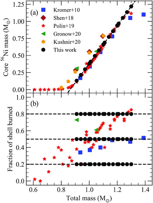
Panel a: 56Ni mass produced in the carbon–oxygen core as a function of total mass of the white dwarf (sum of core and shell mass). Literature values are taken from their respective papers (Kromer et al. 2010; Shen et al. 2018; Polin et al. 2019; Gronow et al. 2020; Kushnir et al. 2020). For total masses between 0.90 and 1.30 M⊙, we show a linear fit to the Polin et al. (2019) models, which is used to determine the core 56Ni mass of our models. Panel b: Fraction of the helium shell that is burned (i.e. converted to elements heavier than helium following the explosion) as a function of total mass. Dashed horizontal lines show fractions of 0.2, 0.5, and 0.8. Black points show the specific models calculated in this work, which broadly extend the range predicted from a variety of explosion models.
In Appendix. B, we present additional models exploring 56Ni masses based on the Shen et al. (2018) and Kushnir et al. (2020) models. Given the uncertainty in the amount of 56Ni produced, the total white dwarf mass should not be taken as a prediction from our models. Throughout this work, we give the values of core and shell masses simply as reference to identify each model. Instead, we consider the total luminosity (i.e. the 56Ni mass) to be a robust prediction and expect that there may be a range of white dwarf properties that produce such a 56Ni mass.
3.2 Composition of the shell
The composition of the helium shell following the explosion remains one of the uncertain properties of double-detonation explosions. The goal of this work is to present models covering a large parameter space and systematically investigate differences in observables that result from various assumptions about the helium shell. In Fig. 3(b), we show the fraction of the helium shell that is burned following the explosion (i.e. converted from helium into heavier elements) for a selection of model sets from the literature. It is clear that there can be a large spread in how much of the shell is consumed, depending on different assumptions made within the models (such as when and how ignition is triggered). To investigate the impact of this on the observables, we choose fractions that bracket those predicted by the different explosion models. Specifically, for each total mass we calculate models for which 20 per cent, 50 per cent, and 80 per cent of the helium shell is burned to other elements. These fractions are shown as black dashed lines in Fig. 3(b), while the individual models calculated in this work are shown as black points.
Aside from simply investigating how much of the shell is burned, we also aim to demonstrate the effects of elements that are produced during shell burning. This is strongly dependent on the initial composition of the shell. Kromer et al. (2010) present a model in which the helium shell is polluted and contains 34 per cent 12C (model 3m). This is shown in Fig. 4, along with the composition of the unpolluted model (model 3). The choice of 34 per cent was specifically made to create a helium shell that is mostly burned to 36Ar, which does not produce strong spectroscopic features. As discussed in other studies (e.g. Shen & Bildsten 2009; Waldman et al. 2011; Gronow et al. 2020), the presence of carbon has an important role to play in regulating helium burning and shaping the nucleosynthetic yields of the helium shell. Therefore, the final composition of the helium shell could be tuned by varying the level of pollution before explosion (Waldman et al. 2011). Piro (2015) has demonstrated that a wide range of carbon pollution fractions could indeed be achieved in the helium shell, depending on specifics of the binary system.
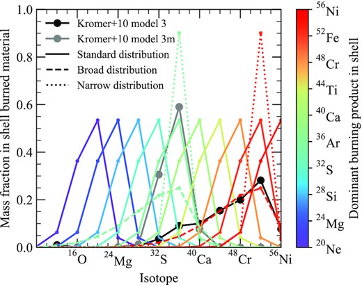
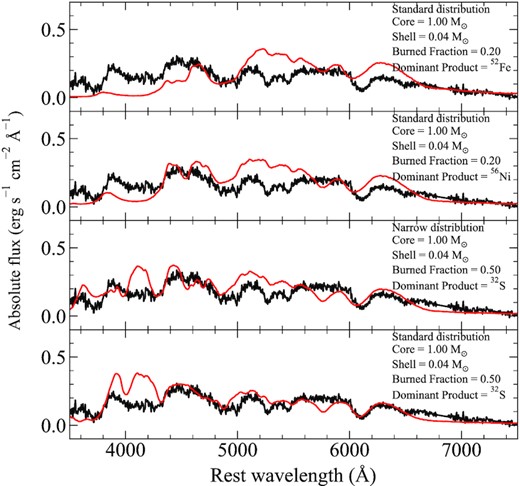
Mass fractions of isotopes along the α-chain produced in the shell. The relative abundances are shown for the Kromer et al. (2010) models assuming a pure helium shell (model 3; black) and a shell that has been polluted with 34 per cent carbon pre-explosion (model 3m; grey). Coloured lines show the mass fractions of all isotopes, assuming burning progresses to a specific point along the α-chain – given by the colour. Solid lines show our standard isotope distributions, based on model 3m. The dashed line shows a broad distribution designed to mimic that of model 3 from Kromer et al. (2010), while the dotted line shows a narrow distribution in which more mass is burned to the dominant shell product.
This picture is complicated further, however, by the presence of other isotopes besides 12C. In particular, Townsley et al. (2019) have shown that α-chain burning can stall at much lower pollution fractions (∼11 per cent) when including 12C, 14N, and 16O. It is clear that the nucleosynthetic yields of the helium shell could show significant variations following explosion. Linking these to specific compositions pre-explosion is a challenging prospect. Therefore, in this study we explore a wide variety of options and assume that burning in the helium shell could stall at any point along the α-chain. We make no claims about specific pre-explosion compositions that could produce such yields. In the following, we refer to the point at which burning stalls as the dominant product in the shell.
We calculate models for dominant shell products ranging from 32S to 56Ni. In our standard model distribution, the relative abundances of other isotopes along the α-chain are taken following from the 3m model of Kromer et al. (2010). We chose model 3m for our standard isotope distribution as it represents an intermediate case to the other distributions explored in this work. In addition, Kromer et al. (2010) present abundances for each isotope produced in the helium shell. Although 36Ar is the dominant shell product in this model, some amounts of other isotopes are produced above and below 36Ar in the chain. This is demonstrated in Fig. 4, which shows that 36Ar is produced with a mass fraction of ∼60 per cent while the previous α-chain isotope (32S) has a mass fraction of ∼30 per cent and the next isotope (40Ca) has a mass fraction of ∼8 per cent. We use a skew normal distribution that approximates the Kromer et al. (2010) 3m distribution in order to determine the relative fraction of all α-chain isotopes, for a given dominant shell product. Explosion models and detailed predicted yields covering a range pollution fractions within the helium shell are currently unavailable. Therefore, assuming that some amounts of isotopes above and below the dominant shell product are also produced seems reasonable. Taking a functional form similar to an existing explosion model is a pragmatic choice, but we note that the exact quantities are unclear.
In Fig. 2(c), we verify that our parametrized approach produces spectra comparable to Kromer et al. (2010). We show a comparison between the maximum light spectrum of model 3 (core mass of 1.025 M⊙, shell mass of 0.055 M⊙) and two of our models with similar parameters (core mass of 1.0 M⊙, shell masses of 0.04 and 0.07 M⊙). In general, our models show similar results; however, the velocities are typically too high. The purpose of Fig. 2(c) is to demonstrate that our parametrized description of the ejecta is not a limiting factor for the method used here. As discussed in Magee et al. (2018), differences in the radiative transfer code used here (turtls) and that of Kromer et al. (2010) (artis; Kromer & Sim 2009) can lead to different observables. This is reflected in the spectra for our models, which are generally bluer than those of Kromer et al. (2010). In addition, the differences in the density profile will have some impact and a combination of these factors appears to result in a shift of features to higher velocities. We again stress that our models are not intended to be reproductions of existing model sets, but are designed to explore a large parameter space. As previously mentioned, by adopting a similar structure to the models of Magee et al. (2020) and Magee & Maguire (2020), we allow for a direct comparison with models from these works, which were all calculated with the same radiative transfer code.
3.3 Alternative abundances in the helium shell
In an effort to quantify the significance of our choice for the relative abundances of isotopes, we calculate two additional sets of models. First, we consider a broad distribution similar to that found for model 3 of Kromer et al. (2010). This corresponds to a higher mass fraction of other isotopes relative to the dominant product in the shell. We also consider a narrow distribution in which the mass fractions of all other isotopes decrease relative to the dominant product. Both cases are shown in Fig. 4 as a dashed and dotted line for a 52Fe- and 36Ar-dominated shell, which are the dominant products produced in the standard model 3 and model 3m of Kromer et al. (2010), respectively.
Together, these two sets of models serve to bracket the distributions assumed throughout this work. The effects of these different compositions are discussed further in the appendix in Section C, but we note that in general the differences are relatively minor.
4 EFFECTS OF POST-EXPLOSION HELIUM SHELL COMPOSITION
In the following section, we discuss the results of our radiative transfer modelling. We demonstrate the significant impact of the helium shell composition on the model light curves and spectra. We compare models with the same core (1.0 M⊙) and shell (0.07 M⊙) masses, but different shell compositions for our standard isotope distribution (Section 3.2, Fig. 4). For this comparison of the effect of different dominant products in the helium shell, we focus on the models in which 50 per cent of the helium shell is burned to heavier elements. Other models within our set show similar variations for different shell compositions.
4.1 Light curves
Fig. 5 shows the effect of the shell composition on the light curve and colour evolution. Similar to previous studies, we find that those models with α-chain burning progressing to IGEs (44Ti–56Ni), which therefore have relatively large amounts of short-lived radioactive isotopes in their shells (56Ni, 52Fe, and 48Cr), display prominent bumps in their light curves within the days following explosion. Although these bumps are most pronounced at shorter wavelengths, they are also clearly seen in redder filters (e.g. r band). Aside from the shape of the light curve, models with IGE-dominated shells also show a distinct colour inversion. The colours are initially blue and quickly reach a peak red colour within a few days of explosion. At this point, the colour evolution turns over and the models become somewhat bluer again, before again turning over and becoming progressively redder towards maximum light.
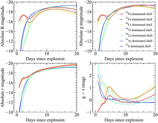
Light curves and colours for models with different shell compositions. All models shown have a 1.0 M⊙ core and a 0.07 M⊙ shell, of which 50 per cent is burned to elements heavier than helium. The dominant α-chain product produced in the shell is given by the colours. The relative fractions of all other isotopes in the shell are given following from Fig. 4.
For those models in which the shell is dominated by IMEs (32S or 36Ar), no early bump is observed due to the lack of the additional radioactive material. Instead, these models show a smooth rise to maximum light, as well as broader and brighter B-band light curves than our IGE-dominated shell models. Our IME-dominated shell models also show a relatively flat colour evolution beginning approximately 5 d after explosion. We have also calculated models for which the assumed α-chain burning stalls earlier than 32S (20Ne, 24Mg, and 28Si); however, these models are very similar to each other and the 32S-dominated model. Therefore, our models show that provided the initial composition of the helium shell is such that burning stops at IMEs, the relative abundances of this burned material are generally unimportant for shaping the evolution of the observables further.
Interestingly, our 40Ca-dominated model represents an intermediate case between the IME- and IGE-dominated shells. No early light-curve bump is observed and the B band in particular shows a longer dark phase (i.e. the time between explosion and the first light emerging from the SN) than all other models. At the same time, the colour evolution does not show an inversion similar to the IGE-dominated shells, but is significantly redder at maximum light compared to the IME-dominated shells. Although 40Ca is the dominant product in the shell (∼55 per cent of the burned material), a small amount of 44Ti is also present (∼5 per cent of the burned material). The additional opacity contribution from 44Ti will act to more effectively blanket the blue flux than in the other IME-dominated shell models, which do not contain 44Ti. On the other hand, the 40Ca-dominated model also lacks a contribution from any radioactive material in the shell, as in the case of the IGE-dominated shell models. Together, both of these properties will cause the lack of additional flux at early times and the redder colours at later times.
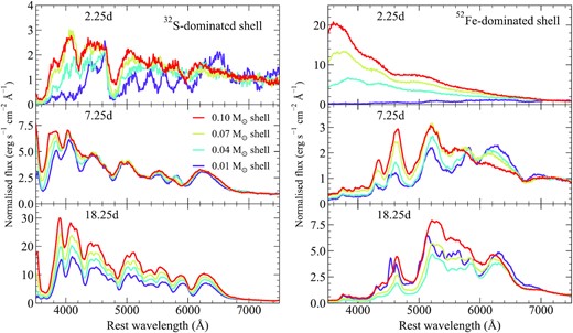
4.2 Spectra
In Fig. 6, we show the spectral evolution of our models with different shell compositions. Spectra are shown at 2.25, 7.25, and 18.25 d after explosion. At 2.25 d after explosion, our models dominated by 56Ni and 52Fe are substantially bluer than all other models and show relatively featureless spectra. Despite still containing short-lived isotopes near the surface of the ejecta, Fig. 6 shows that our 48Cr-dominated model spectrum is much redder than either the 56Ni- or 52Fe-dominated model spectra. As shown in Fig. 1, 52Fe is the dominant source of luminosity for the early light-curve bump – due to its short half-life. Although some 52Fe is present in the shell of our 48Cr-dominated model, it has a much lower fraction than that in the 56Ni- or 52Fe-dominated models – hence there is a lower luminosity and less heating, producing a fainter and redder spectrum during the early bump. Our 48Cr-dominated spectrum also shows a strong absorption feature due to S ii at ∼4800 Å. At 2.25 d, our IME-dominated models are still in the dark phase (i.e. very little luminosity has actually escaped). Despite their low luminosity, a weak Si ii λ6355 feature is still visible in our 36Ar- and 32S-dominated models, as well as the S ii feature around ∼4800 Å that is also visible in our 48Cr-dominated model.
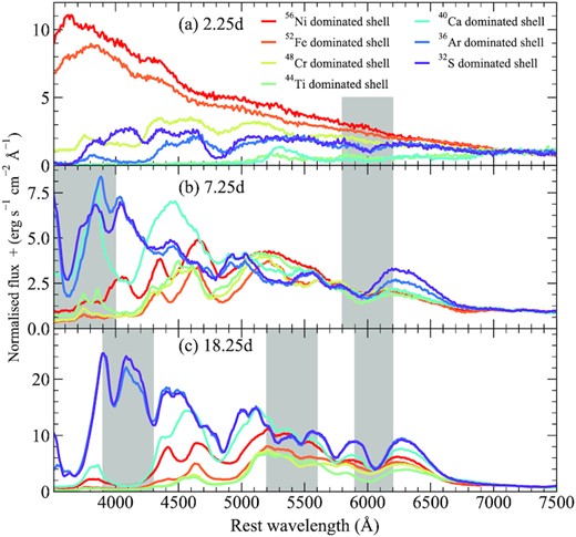
Spectra for models with different shell compositions. All models shown have a 1.0 M⊙ core and a 0.07 M⊙ shell, of which 50 per cent is burned to elements heavier than helium. The dominant α-chain product produced in the shell is given by the colours. The relative fractions of all other isotopes in the shell are given following from Fig. 4. Spectra are shown at three epochs: 2.25, 7.25, and 18.25 d after explosion. All spectra are normalized to the flux between 7000 and 7500 Å. Features discussed in the main text are shown as shaded regions.
One week after explosion, the 56Ni- and 48Cr-dominated shell models have become significantly redder. Much of the flux below ≲4000 Å has been blanketed out in all models with IGE-dominated shells. These models also show a broad absorption feature due to Ti ii around ∼4200 Å (with the exception of the 56Ni-dominated model, which does not contain Ti in the shell). Our 48Cr model shows remarkably little spectral evolution between the two epochs presented here relative to other models within our set. In the IGE-dominated models, a few additional features are produced at longer wavelengths (most notably the Si ii λ6355 feature), but in general they are weaker and broader than those in models that do not contain IGE in the shell. For our 36Ar- and 32S-dominated models, the spectra are now considerably bluer than the IGE-dominated models. Absorption profiles due to IME, such as Si ii λ6355 and the S ii-W feature, can be observed. Both models also show strong Ca ii absorption at ∼3600 Å.
Moving to maximum light, more of the blue flux in our IGE-dominated models has been blanketed out. At this epoch, the spectra show very little flux below ∼4300 Å and again show a broad, flat Ti ii profile between ∼3900 and 4300 Å. Around ∼4700–4900 Å, the IGE-dominated models show a similarly broad and flat feature due to Cr ii and Ti ii. For these models, features due to IME (Si ii λ6355, Si ii λ5972, and S ii-W) are again broader and weaker than those in the IME-dominated shell models.
High-velocity features have been reported in a number of SNe Ia at early times (e.g. Childress et al. 2014; Maguire et al. 2014; Zhao et al. 2015). The origin of these features is unclear, but one proposed scenario is from an abundance or density enhancement that may be due to circumstellar interaction or intrinsic to SN itself (Mazzali et al. 2005; Tanaka et al. 2008). Double-detonation models producing IMEs in the helium shell would be a natural method producing such an abundance enhancement. To investigate whether our IME-dominated shells produce similar features and if these can be attributed to high-velocity material in the shell, we calculate the contribution of the shell material to the synthetic spectra. During the simulation, we track the location at which a Monte Carlo packet experiences its last interaction. In Fig. 7, we show separate spectra produced by binning Monte Carlo packets that last interacted with material in either the shell or the core. We note that we are only able to track the location of real packets (rather than virtual packets; see Magee & Maguire 2020); therefore, the signal-to-noise ratio of these spectra is lower than others presented throughout this work. Nevertheless, Fig. 7 shows that within the first approximately 1 week since explosion, the shell material does contribute to the production of high-velocity features. Specifically, the Si ii λ6355 feature is shifted to higher velocities and broadened when including contributions from the shell. Around maximum light, however, there is a negligible impact from the shell material. While our models indicate that helium shell ash could provide one explanation for high-velocity features seen in some SNe Ia at early times, further modelling work is required to fully constrain the abundance profiles required.
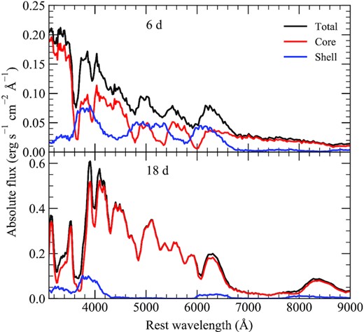
Contribution of material in the helium shell and core to the observed spectra at different phases. Spectra are calculated by binning packets separately, depending on the location of their last interaction.
4.3 Summary
Our models clearly show the impact of the post-explosion helium shell composition on the observables. Those models in which the shell is burned mainly to IGE show an early bump in the light curve, a colour inversion, and significantly reddened spectra from approximately 1 week after explosion. Conversely, our models in which the shell mostly contains IMEs do not show an early bump and instead have a relatively flat colour evolution. In addition, we find that as long as burning within the shell does not progress to IGEs, the model observables show much smaller variations than those for which the shell is dominated by IGEs. This would indicate that meticulous fine-tuning is not necessary to avoid the impact of the helium shell ash on the observables – provided burning ceases at a certain point, the exact composition of the shell is mostly irrelevant.
5 EFFECTS OF THE BURNED MASS
In this section, we demonstrate how the amount of burned material above the core affects the model observables. To focus our discussion, we limit our comparisons to models with a core mass of 1.0 M⊙. Our models are controlled by both the mass of helium shell and the amount of the shell that is assumed to be burned during the explosion. As the mass of the helium shell also determines the amount of 56Ni produced during the explosion, which will have a significant impact on the model observables, it is not possible to explore solely the effect of the total amount of material burned. Therefore, in Section 5.1 we discuss the effects of the helium shell mass and in Section 5.2 we discuss the role of the burned fraction.
5.1 Impact of helium shell mass on light curves and spectra
In Fig. 8, we show the light curve and colour evolution for models with varying shell masses, while the spectral evolution is shown in Fig. 9. We limit our comparison to the 52Fe- and 32S-dominated shells, which are representative of trends observed for IGE- and IME-dominated shells, respectively (see Section 4).
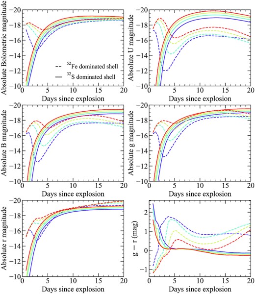
Light curves and colours for models with different shell masses. All models shown have a 1.0 M⊙ core and we assume that 80 per cent of the shell is burned to elements heavier than helium. We show two representative cases in which the composition of the shell is dominated by either 32S or 52Fe.
Spectra for models with different shell masses. All models shown have a 1.0 M⊙ core and we assume that 80 per cent of the shell is burned to elements heavier than helium. We show two representative cases in which the composition of the shell is dominated by either 32S or 52Fe. Spectra are shown at three epochs: 2.25, 7.25, and 18.25 d after explosion. All spectra are normalized to the flux between 7000 and 7500 Å.
As discussed in Section 4, our 32S-dominated shell models do not produce an early bump in the light curve, but there is still some variation among the different shell masses. This is not primarily driven by material in the shell, but rather the different 56Ni masses in the core of the white dwarf (Section 3.1, Fig. 3). Therefore, models with more massive shells are brighter and somewhat bluer simply due to the increased ejecta mass and hence 56Ni mass. Fig. 9 shows that these models also produce similar spectra, with the primary differences being the luminosity and colour. Differences between the spectra of models with different shell masses are most pronounced at early times, where lower mass shells show stronger Si ii and S ii features, likely due to their lower temperatures. For our IME-dominated models we also note that there is also a degeneracy between the core and shell masses. For the models presented here, provided the total ejecta mass is the same, the distinction between the core and shell is unimportant. For example, our 32S-dominated model with a 1.0 M⊙ core and a 0.1 M⊙ shell and model with a 1.1 M⊙ core and a 0.01 M⊙ shell produce similar light curves and spectra.
For our 52Fe-dominated shells, Fig. 8 shows that all models produce a light-curve bump. The time-scale of the bump varies significantly (∼1–5 d) for the broad-band light curves, with lower mass shells producing shorter lived and more rapidly evolving bumps. As demonstrated by Fig. 8, this is primarily due to temperature evolution for the different models, as there is significantly smaller spread in the bump time-scales in bolometric light. Unlike the 32S-dominated shell models, the shell mass has a considerable impact on the colour evolution for the 52Fe-dominated models. Smaller shell masses produce a more rapid and extreme change in colour within the first 5 d after explosion. In addition, beginning approximately 10 d after explosion, the lowest mass shell model (0.01 M⊙) shows a relatively flat colour evolution towards maximum light. In contrast, models with more massive shells become significantly redder over this same period. The 0.10 M⊙ shell model remains redder than both the 0.07 and 0.04 M⊙ shell models for all times presented here; however, the overall difference between their respective colours decreases with time. This likely points to two competing effects – the influence of line blanketing from the shell and the different 56Ni masses causing different temperatures. More massive shells will produce more line blanketing and hence one may expect redder colours, but this is not observed for the models presented here. In this case, as the core mass is the same, the increase in the shell mass results in an increased 56Ni mass that keeps the ejecta hotter and bluer. Fig. 9(d) shows that, at 2.25 d after explosion, the temperature is the primary difference between the models and few features are present. At later epochs, our models show that larger shell masses produce broader Si ii λ6355 features and weaker IME features overall.
5.2 Impact of the burned fraction percentage on light curves and spectra
The amount of material in the shell converted from helium to heavier elements is also a free parameter of our models. We have investigated burned fractions of 20 per cent, 50 per cent, and 80 per cent, which approximately span the range predicted by different explosion models (see Fig. 3b). The differences between these models are fairly straightforward and follow the trends one may expect. For IME-dominated shell models, the burned fraction has no effect on the resultant observables. For IGE-dominated shell models, a higher burned fraction will result in a brighter bump at early times and redder colours at later times.
6 MODEL RISE TIMES AND BUMP TIME-SCALES
Here, we discuss the rise times and peak magnitudes of the models presented in this work and demonstrate the range of magnitudes and time-scales for early light-curve bumps. In Fig. 10(a), we show the B-band rise times and peak absolute B-band magnitudes for our models with the standard isotope distribution. The difference between our IGE- and IME-dominated shell models is readily apparent. We find that, in general, those models with IGE-dominated shells show shorter rises, with a median rise time of 13.8 ± 2.3 d, compared to those with IME-dominated shells, which have a median rise time of 17.6 ± 0.7 d. The longer rise time of the IME-dominated models is more typical of normal SNe Ia (e.g. Ganeshalingam, Li & Filippenko 2011; Firth et al. 2015; Miller et al. 2020a). Although in general we find that models with IGE-dominated shells show shorter rise times, there are some notable exceptions. For a 0.9 M⊙ core, some models with low-mass shells (0.01 and 0.04 M⊙) can show longer rise times than similar models with higher mass cores. In these cases, the longer rise times result from a combination of the compact 56Ni distribution and less extreme line blanketing of the low-mass shell. For our IME-dominated models, the scatter in the peak absolute B-band magnitude is driven simply by differences in 56Ni mass due to the various core and shell masses explored here. Models with IGE-dominated shells, however, show a significantly larger scatter (≳4 mag compared to ∼2 mag for IME-dominated shells) due to line blanketing from the material in the shell. Indeed, at longer wavelengths that are less sensitive to line blanketing (e.g. r band), both the IGE- and IME-dominated shell models show a similar scatter in peak magnitudes (again, due to the differences in the 56Ni mass), although the IGE-dominated models are systematically brighter as much of the blue flux has been reprocessed to longer wavelengths by the shell.
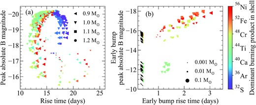
Panel a: Peak absolute B-band magnitudes against rise time to peak B-band magnitude. Panel b: Peak absolute B-band magnitudes of the early light-curve bump against time to reach the peak of the bump. We note that all models with IME-dominated shells and some models with high core masses do not show early bumps and therefore are neglected. For models in which the light curve is already declining at the start of our simulation (0.5 d), we consider these as upper limits and show them as black arrows. In both panels, each model is coloured based on the dominant element produced in the shell. The size of each point is proportional to the burned mass of the helium shell (i.e. the product of the shell mass and burned fraction), while the shape of each point denotes the mass of the core.
Fig. 10(b) shows the properties of the early light-curve bumps. We calculate the time since explosion to reach the peak of the bump and the magnitude at this point. For some models, the light curve is already declining at the beginning of our simulations (0.5 d after explosion). We therefore consider these points as limits and show them as black arrows in Fig. 10(b). We do not include models with IME-dominated shells as they do not show a bump at early times. In addition, some models, such as those with large total masses (≳1.2 M⊙), do not show pronounced bumps in their light curves due to their high 56Ni masses and extended distributions. In other words, there is no clear decline in the light curve within the first few days of explosion. These models are also not included in Fig. 10(b). Among the models shown in Fig. 10(b), there is a general trend that brighter bumps are also typically longer lasting. Models with 44Ti-dominated shells, however, deviate from this trend. Following from Fig. 4, in our 44Ti-dominated model only a small amount of 48Cr is contained within the shell. Therefore, this set of models contains a significantly smaller mass of radioactive isotopes in the shell compared to our other IGE-dominated models. We also note that the models shown as limits in Fig. 10(b) hint at the possibility of bright and very short lived bumps – less than 0.5 d. It is highly likely that such bumps could be missed in most current surveys.
7 COMPARISON WITH A CHANDRASEKHAR-MASS MODEL CONTAINING A 56NI EXCESS
Magee & Maguire (2020) present light curves and spectra of Chandrasekhar-mass models that contain an excess of 56Ni (a 56Ni shell) in the outer ejecta. Qualitatively, these models show similar behaviour (light-curve bumps at early times and line blanketing closer to maximum light) to double detonations in which a significant fraction of IGEs are produced in the shell. Here, we perform a comparison between these two cases and investigate ways in which they may be distinguished from each other, based on the early light-curve bump and spectra at maximum light.
In Fig. 11(a), we show the 56Ni distributions of Chandrasekhar-mass model with and without a 56Ni excess compared to the sub-Chandrasekhar double-detonation models explored in this work. We show one of the Chandrasekhar-mass models from Magee & Maguire (2020) that does not contain a 56Ni excess (black in Fig. 11; described as the fiducial SN 2018oh model in Magee & Maguire 2020), along with a model in which a 0.03 M⊙56Ni shell has been added to the outer ejecta (Fig. 11, green). We present an additional Chandrasekhar-mass model without a 56Ni excess, but in which the 56Ni distribution has been extended, such that 56Ni is present throughout the ejecta with a mass fraction that decreases monotonically towards the outer ejecta (Fig. 11, grey). For our sub-Chandrasekhar-mass double-detonation model with a 1.0 M⊙ core and a 0.07 M⊙ shell dominated by 56Ni (WD1.00_He0.07_BF0.50_DP56Ni; Fig. 11, red), the total 56Ni mass and 56Ni distribution in the outer ejecta are similar to the 56Ni excess model. Finally, we also show the same model with a 32S-dominated shell (WD1.00_He0.07_BF0.50_DP32S; Fig. 11, blue) as representative of a sub-Chandrasekhar-mass model without an excess of 56Ni in the outer ejecta. We note that the density profile and ejecta mass differ slightly between the double-detonation and Chandrasekhar-mass models shown here.
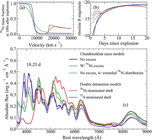
Panel a: Comparison between the 56Ni distributions for models presented here. We show a Chandrasekhar-mass model from Magee & Maguire (2020) that contains a 56Ni excess in the outer ejecta and the corresponding model without an excess, in addition to a model with an extended 56Ni distribution. Double-detonation models with a 56Ni- and 32S-dominated shell (red and purple, respectively) are also shown. Panel b: B-band light curve for models presented here. Panel c: Comparison of spectra for our models at 18.25 d after explosion.
Fig. 11(b) demonstrates that the sub-Chandrasekhar-mass double-detonation 56Ni-dominated shell model shows a more pronounced bump that rises and declines within a few days compared to the more plateau-like shape of the Chandrasekhar-mass 56Ni excess model. Even for double-detonation models with a lower 56Ni mass fraction in the outer ejecta (i.e. different burned fractions), the 56Ni-dominated shells do not reproduce the shape of the 56Ni excess models. Such a difference in light-curve shape, despite similar 56Ni distributions, serves to further highlight the importance of the additional radioactive isotopes produced in the double-detonation models. For the Chandrasekhar-mass 56Ni excess model, 56Ni is the only radioactive isotope considered in the ejecta, while the double-detonation model also contains 52Fe and a small amount of 48Cr. Hence, the bump produced in the light curve of the 56Ni-dominated shell model is more pronounced due to the presence of 52Fe, 52Mn, and 48Cr, which have considerably shorter half-lives compared to 56Ni. At later epochs, the double-detonation model with a 56Ni-dominated shell becomes significantly redder and fainter than the 56Ni excess model. Again, this points to important differences in the ejecta composition – the presence of additional IGEs in the double-detonation model will more effectively blanket blue flux than just the 56Ni decay chain as in the 56Ni excess model. For our 32S-dominated shell model, the light curve shows a sharper rise and slightly longer dark phase than the model without a clump. In this case, the 56Ni distribution is somewhat less extended and shows a more rapid change from 56Ni-rich to 56Ni-poor ejecta than the Chandrasekhar-mass model without a 56Ni excess.
In Fig. 11(c), we show the spectra of all models at 18.25 d after explosion. At this epoch, our Chandrasekhar-mass model without a 56Ni excess and 32S-dominated shell model show extremely similar spectra (black and purple lines), with the most noticeable difference being that the double-detonation model is marginally bluer. Conversely, the 56Ni-dominated shell model (red line) is significantly different from all other models, including the Chandrasekhar-mass 56Ni excess model (green line). The flux below ∼4000 Å is essentially completely removed from the spectrum and redistributed to wavelengths ≳5000 Å, which show a significantly higher continuum flux. The Cr ii and Ti ii features present in the double-detonation model at ∼4000–5000 Å easily distinguish it from the 56Ni excess model.
Comparing Chandrasekhar-mass models with a 56Ni excess in the outer ejecta and sub-Chandrasekhar-mass double-detonation models in which a 56Ni-dominated shell is produced as a result of helium shell burning, we find that the two are easily distinguished despite qualitatively similar behaviour. Although thought to be created via a different mechanism, models with 56Ni excess can also produce an early light-curve bump. The shape of the bump, however, more closely resembles a plateau compared to the clear peak in the double-detonation models. The significant amount of IGEs produced during helium shell burning leads to extremely red colours – even more so than the 56Ni excess models, which also show red colours at maximum. Finally, our IGE-dominated shell models also show shorter rise times than the 56Ni excess models of Magee & Maguire (2020).
8 COMPARISONS WITH NORMAL SNE IA
In the following section, we discuss whether our double-detonation models are consistent with observations of SNe Ia. We compare to light curves and spectra of two well-observed and prototypical SNe Ia, namely SNe 2011fe (Nugent et al. 2011; Richmond & Smith 2012; Vinkó et al. 2012) and 2005cf (Garavini et al. 2007; Pastorello et al. 2007). Fig. 12 shows the light curves of both objects compared to our models, while spectra are shown in Fig. 13. For SN 2011fe, we show a model with a 1.0 M⊙ core and a 0.04 M⊙ shell dominated by sulphur (WD1.00_He0.04_BF0.20_DP32S). The 56Ni mass of this model (0.49 M⊙) is comparable to estimates for SN 2011fe (∼0.45 M⊙; Nugent et al. 2011). For SN 2005cf, we find that a larger total mass is required to reproduce the higher core 56Ni mass (0.7 M⊙; Pastorello et al. 2007). Our models with either a 1.0 M⊙ core and a 0.10 M⊙ shell or a 1.1 M⊙ core and a 0.01 M⊙ shell both produce similar light curves and spectra for a 32S-dominated shell and may be considered interchangeable. Here, we present the model with a 1.0 M⊙ core and a 0.10 M⊙ shell for SN 2005cf. As previously mentioned (Section 3.1), there is disagreement between various studies over the amount of 56Ni produced for a given white dwarf mass during explosion. For this reason, the core and shell masses presented here should not be taken as predictions for the objects discussed here, but are simply given as reference to identify the comparison models shown. SN 2011fe has been corrected for a total extinction of E(B − V) = 0.01 mag (Nugent et al. 2011), while SN 2005cf has been corrected for E(B − V) = 0.1 mag (Pastorello et al. 2007).
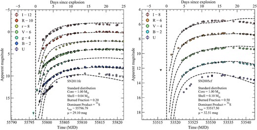
Comparisons between the optical light curves of SNe 2011fe and 2005cf (coloured circles) and our sub-Chandrasekhar double-detonation model light curves (dashed black lines). The model parameters and assumed distance modulus are given for each object. The estimated time of explosion (based on the comparison with the model light curve) is shown as a vertical dashed line for each SN.
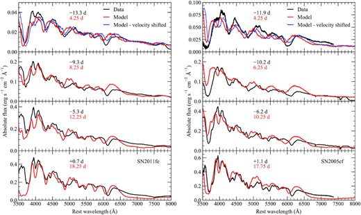
Comparisons between spectra of SNe 2011fe and 2005cf (black), and our double-detonation models with 32S-dominated shells (red) at epochs from 4 to 18 d after explosion, along with the parameters of both models. Spectra are shown on an absolute flux scale. For the first epoch, we also show model spectra shifted in velocity to provide better agreement to the observed features (blue). The phases of the observed spectra of SNe 2011fe and 2005cf relative to B-band maximum are given in black, while the time since explosion for our model comparison spectra is shown in red.
Fig. 12 demonstrates that our double-detonation models with 32S-dominated shells provide good agreement with the light-curve shapes of both objects beginning a few days after explosion and extending to approximately maximum light. The largest discrepancies between models and observations are observed in the U band, but we note this is likely related to the simplified composition and ejecta structure used (see Magee et al. 2020), and will be explored in future work. Townsley et al. (2019) have also previously shown that a double-detonation model with a 1.0 M⊙ core and a 0.02 M⊙ helium shell dominated by IMEs can reproduce the light curve of SN 2011fe. For epochs ≲4 d after explosion, however, both models clearly show a rise that is too sharp and a dark phase that is too long to match the observed flux. By comparing to several Chandrasekhar-mass models of different 56Ni distributions, Magee et al. (2020) found that the early light-curve points of SN 2011fe can be reproduced by a relatively extended 56Ni distribution with a mass fraction in the outer ejecta of ∼0.03. In contrast, the double-detonation models shown here, which have 32S-dominated shells, do not contain any 56Ni in the outer ejecta. As shown in Fig. 2, the functional form used for the models presented here produces a 56Ni distribution that is somewhat more compact than that predicted by Kromer et al. (2010). A slightly more extended core 56Ni distribution for the double-detonation models with 32S-dominated shells could likely reproduce the earliest detections of SNe 2011fe and 2005cf, without adversely affecting the light curve at later times.
Fig. 13 shows a comparison between the spectra of SNe 2011fe and 2005cf and their corresponding double-detonation models with 32S-dominated shells. Previous comparisons to double-detonation and bare sub-Chandrasekhar-mass models have focused only on spectra around maximum light. Here, we show spectra for both objects at multiple epochs, beginning ∼4 d after explosion and extending to maximum light. For our double-detonation models, we find that spectra at 4.25 d after explosion are consistent with those of both objects approximately 2 weeks before maximum. Although many of the features are reproduced with approximately the correct strength and shape, such as Si ii λλ6355 and 5972, S ii-W, Mg ii λ4481, O i λ7774, and the Ca ii NIR triplet, they are all noticeably offset to higher velocities in the models compared to the observed spectra. Therefore, in Fig. 13, we also show our model spectra with a velocity shift of ∼6000 km s−1 applied and find improved agreement. As discussed in Section 3.2, the systematic shift to high velocities in our spectra could be due to simplifications made in our model density profiles, particularly in the outer regions. Closer to maximum light, velocities of many features (such as the S ii-W feature) in our model spectra show good agreement with both SNe, although Si ii velocities are still somewhat higher than those observed. In Section 4, we show how the material in the helium shell can impact the spectroscopic features within the first week of explosion. Qualitatively, this is similar to the broad Si ii λ6355 feature in SN 2005cf, which has been argued to have a high-velocity component (Garavini et al. 2007). Again, we note that there is a systematic shift of all features to higher velocities at this time. Nevertheless, our models provide tentative evidence that the high-velocity components in some SNe Ia may be due to interactions with a helium shell containing IMEs.
Our models verify the claims of Kromer et al. (2010) and Townsley et al. (2019) that double-detonation explosions in which the helium shell does not produce significant fractions of IGE are consistent with the observed behaviour of normal SNe Ia and therefore cannot be ruled out on this basis. Here, we extend this to show that models with different helium shell masses are also capable of reproducing multiple normal SNe Ia and at various epochs up to maximum light. While our models generally show good agreement from a few days after explosion, the initial rise of the light curve is sharper than observed, supporting the claims of Magee et al. (2020) that a more extended distribution for 56Ni in the core may be required.
9 COMPARISONS WITH SNE IA SHOWING AN EARLY LIGHT-CURVE BUMP
A handful of objects with early light-curve bumps have now been discovered. Among these objects, two distinct groups are clearly apparent based on their optical colour close to maximum light – those that are extremely red, with B − V ≳ 1 (SNe 2016jhr, 2018byg), and those that are relatively normal with a blue colour, B − V ≲ 1 (SNe 2017cbv, 2018oh, 2019yvq, and iPTF14atg). In Section 9.3, we discuss the case of PTF10ops separately, which has been suggested to show excess flux at early times (Jiang et al. 2018), but its true nature is unclear due to a limited data set. In the following sections, we compare our models to observations of SNe Ia with early bumps split into ‘blue’ and ‘red’ SN sub-classes, and discuss our models in the context of other scenarios that have been proposed for these objects.
Again, we stress that exact values for the core mass should not be taken literally due to the uncertainty in the amount of 56Ni produced (Section 3.1), but are given for reference. The shell masses presented here are likely more robust predictions as our models cover a wide range of burned masses and products, and the observed shape of the bump will be highly sensitive to the mass of the shell.
9.1 Blue SNe Ia with an early bump
Fig. 14 shows a comparison between the light curves of SNe 2017cbv, 2018oh, 2019yvq, and iPTF14atg, and four of our double-detonation models with 56Ni-dominated shells. These models are broadly able to reproduce the shape of the early light-curve bump. In Fig. 15, we compare spectra of each SN and model around maximum light.
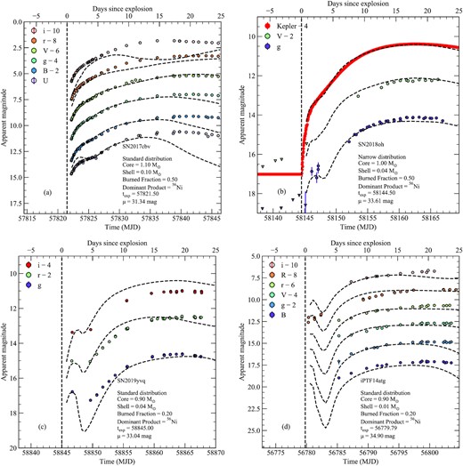
Comparisons between SNe 2017cbv, 2018oh, 2019yvq, and iPTF14atg (coloured circles) and our double-detonation models (dashed lines) with 56Ni-dominated shells. The model parameters and assumed distance modulus are given for each object. The estimated time of explosion (based on the comparison with the model light curve) is also shown as a vertical dashed line for each SN.
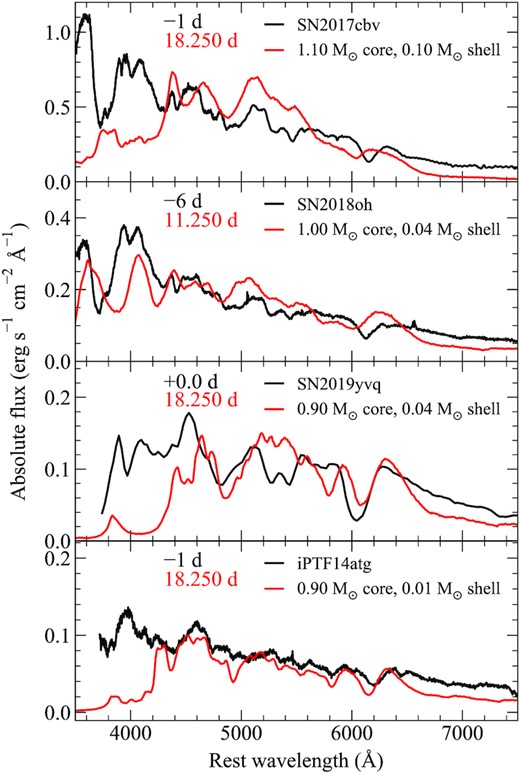
Comparisons between SNe 2017cbv, 2018oh, 2019yvq, and iPTF14atg (black) and our model spectra (red) around maximum light, along with the parameters of all models. Spectra are shown on an absolute flux scale. Phases of SNe relative to B-band maximum are given in black, while the time since explosion for our model spectra is shown in red.
The light curve of SN 2017cbv was previously compared to double-detonation models by Maeda et al. (2018); however, their models were somewhat too faint (SN 2017cbv was a bright SN Ia and showed a peak absolute magnitude of MB = −20.4; Hosseinzadeh et al. 2017). In Fig. 14(a), we show that our model with a 1.1 M⊙ core and a massive helium shell of 0.10 M⊙ dominated by 56Ni can generally reproduce the shape of the early light curve of SN 2017cbv. The 56Ni mass of this model is 0.94 M⊙. For the model shown in Fig. 14(a), the U band shows a more pronounced bump than observed; we speculate that minor changes to the composition within the helium shell could be made to find improved agreement in this band. Regardless of this discrepancy, beginning approximately 3 weeks after explosion the model light curves show a much faster decline in the bluer bands (U, B, and g) than SN 2017cbv. This is further demonstrated by Fig. 15, which shows that the maximum light spectrum of our double-detonation model with a 56Ni-dominated shell exhibits significant line blanketing that is inconsistent with SN 2017cbv. In addition, the spectral features are also inconsistent with SN 2017cbv. Our model shows a significantly broadened Si ii λ6355 feature that has blended with Si ii λ5972. In contrast, the observed spectra of SN 2017cbv show a well-defined Si ii λ6355 feature and lack Si ii λ5972.
Hosseinzadeh et al. (2017) compare observations of SN 2017cbv to models of the interaction between the SN ejecta and a non-degenerate companion star. While they find that interaction with a 56 R⊙ sub-giant is able to reproduce the bump in the optical bands, the model overpredicts the flux in the ultraviolet (UV) bands (UVW1, UVM2, and UVW2). Hosseinzadeh et al. (2017) argue that this could indicate that the flux resulting from the interaction is not a blackbody or an alternative explanation is required. Based on nebular spectra hundreds of days after explosion, Sand et al. (2018) rule out the presence of any significant H α signatures, which are expected if material is stripped from a non-degenerate companion. Finally, the presence of CSM was also ruled out by Ferretti et al. (2017). Our models indicate that SN 2017cbv likely did not result from a double-detonation explosion. Taken together, the nature of SN 2017cbv is still uncertain.
Dimitriadis et al. (2019) compare SN 2018oh to a double-detonation explosion model with a 0.98 M⊙ core and a 0.05 M⊙ helium shell, which produces 0.45 M⊙ of 56Ni. To match the early light-curve bump of SN 2018oh, Dimitriadis et al. (2019) invoke mixing of the SN ejecta after explosion. Therefore, the model does not produce a well-defined early bump in the light curve, but rather shows an extended ‘shoulder’ that more closely resembles SN 2018oh. It is not clear, however, whether such mixing could be achieved in double-detonation explosions. Fig. 14(b) shows that our model with a 1.0 M⊙ core and a thin helium shell of 0.04 M⊙ (i.e. a 56Ni mass of 0.49 M⊙) with a narrow isotope distribution dominated by 56Ni provides reasonable agreement to the light-curve shape of SN 2018oh. A narrow isotope distribution is required to reduce the mass of 52Fe in the shell and avoid the peak produced by its short lifetime. Even for this distribution, however, the bump in the model Kepler-band light curve is more pronounced than that observed in SN 2018oh. Reducing the 52Fe mass further may again provide improved agreement as Magee & Maguire (2020) have shown that the light-curve bump in SN 2018oh can be reproduced by a model containing a clump of pure 56Ni in the outer ejecta.
Although this model is less affected by line blanketing than the model for SN 2017cbv, due to the lower mass of the helium shell, Fig. 15 shows that the spectral features of SN 2018oh are also inconsistent with a double-detonation scenario. Dimitriadis et al. (2019) did not consider the spectra of their double-detonation models compared to SN 2018oh. In summary, our models indicate that SN 2018oh did not result from a double-detonation explosion as we are unable to simultaneously match the spectroscopic features and early light-curve bump, regardless of the composition of the helium shell.
Dimitriadis et al. (2019) slightly favour an interpreation for SN 2018oh as resulting from interaction with a non-degenerate companion. Again, similar to SN 2017cbv, no evidence for material stripped from a non-degenerate companion has been found in late-time spectra of SN 2018oh (Dimitriadis et al. 2019; Tucker, Shappee & Wisniewski 2019). The case of interaction with CSM was investigated by Shappee et al. (2019), who found that none of their interaction models could satisfactorily reproduce the initial early light-curve shape of SN 2018oh. An alternative case of interaction for SN 2018oh was suggested by Levanon & Soker (2019). In this scenario, the explosion follows from the merger of two white dwarfs. An accretion disc forms around the primary (Raskin et al. 2012; Zhu et al. 2013), which serves as the source of the CSM. After explosion, the SN ejecta shock material in the disc, producing a flash of UV radiation that may be similar to that of SN 2018oh (Levanon, Soker & García-Berro 2015). This scenario warrants further investigation with radiative transfer simulations, as alternatives appear to be ruled out for SN 2018oh.
In Fig. 14(c), we compare a double-detonation model to SN 2019yvq (Miller et al. 2020a). SN 2019yvq was a somewhat peculiar SN – it was slightly underluminous, but showed high-velocity spectral features. Miller et al. (2020a) compared observations of SN 2019yvq to a variety of models, including double-detonation explosions. They found reasonable agreement to a double-detonation model with a 0.92 M⊙ core and a 0.04 M⊙ shell. In Fig. 14(c), we show our model with comparable values – a 0.9 M⊙ core and a 0.04 M⊙ shell dominated by 56Ni. The similarity of these values is unsurprising, given that Miller et al. (2020a) use the same modelling treatment as Polin et al. (2019), upon which our models are at least partially based. As in Miller et al. (2020a), our model generally matches the early light-curve bump in the redder bands (r and i), but the g band shows a larger decrease in magnitude than what is observed immediately following the peak of the bump. Even for models with different dominant products (e.g. 52Fe and 48Cr) in the shell, we are not able to simultaneously match the bump in both the g and r bands. As with SNe 2017cbv and 2018oh, Fig. 15 shows that the maximum light spectrum of SN 2019yvq is significantly bluer than the model and does not exhibit strong line blanketing.
In addition to double-detonation explosions, Miller et al. (2020a) investigate other scenarios to explain SN 2019yvq, including an excess of 56Ni in the outer ejecta, a violent merger, and companion interaction. None of the proposed scenarios fully explain all of the observed features. One possible exception is the violent merger scenario. While it is likely that this scenario does produce some CSM, models including this material are currently unavailable. Based on the identification of calcium in nebular spectra and favourable comparisons with model nebular spectra, Siebert et al. (2020) argue that SN 2019yvq was indeed the result of a helium shell detonation. The light curve of the model favoured by Siebert et al. (2020), however, does not reproduce what is observed in SN 2019yvq. The model is simultaneously too bright and does not show a pronounced bump at early times. Whether it is possible to simultaneously match the early- and late-time observations of SN 2019yvq requires further investigation.
Finally, Fig. 14(d) shows iPTF14atg compared to a double-detonation model with a 0.9 M⊙ core and a thin helium shell of 0.01 M⊙. This model contains only 0.13 M⊙ of 56Ni. Unlike the other objects discussed here, the early bump observed in iPTF14atg was less pronounced in the optical bands, but clearly apparent at UV wavelengths. (Cao et al. 2015). The origin of this early excess was discussed by Cao et al. (2015), who argued that it is consistent with theoretical predictions of the collision between the SN ejecta and companion star. They also discuss the possibility of this excess arising from 56Ni at the surface of the ejecta, such as in double-detonation models, and estimate that this would require a 56Ni mass of ∼0.01 M⊙ at the surface. Fig. 14(d) shows that even for our model with a 0.01 M⊙ shell, the early light-curve bump produced is inconsistent with iPTF14atg. Fig. 15 also shows the maximum light spectrum of iPTF14atg. Our model predicts a spectrum at maximum light that is substantially redder than iPTF14atg, and shows strong flux suppression for wavelengths ≲4200 Å. The origin of iPTF14atg was also considered by Kromer et al. (2016), who favour the violent merger of two white dwarfs. This particular realization of the violent merger scenario did not predict a light-curve bump, but interaction due to the presence of some CSM for similar models may be consistent with the observations.
9.2 Red SNe Ia with an early bump
Observations of SN 2016jhr were presented by Jiang et al. (2017), who found reasonable agreement with models of double detonations and either sub- or near-Chandrasekhar-mass white dwarfs. In Fig. 16, we show a comparison between some of our double-detonation models and SN 2016jhr. We note that unlike Jiang et al. (2017), we do not apply K-corrections to the observed light curve as these may be uncertain due to the peculiar nature of SN 2016jhr. Instead, we transform our model spectra into the observer frame (redshift of 0.117) and calculate observer frame light curves. For all comparisons, we assume an explosion date of MJD = 57482.0, which is a few hours before the first detection. We also assume a distance modulus of μ = 38.99 mag, which is 0.3 mag higher than that used by Jiang et al. (2017).
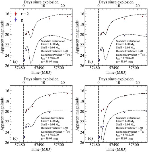
Comparisons between SN 2016jhr and a subset of our models. The model parameters and assumed distance modulus are given for each object. The estimated time of explosion (based on agreement with the model light curve) is also shown as a vertical dashed line for each SN. In all cases, our model light curves have been transformed into the observer frame of SN 2016jhr (redshift of 0.117).
Fig. 16(a) shows our model with a 1.0 M⊙ core and a 0.04 M⊙ helium shell dominated by 52Fe. The core and shell masses of models shown here are comparable to the models presented by Jiang et al. (2017) (1.03 M⊙ core and 0.054 M⊙ helium shell) and Polin et al. (2019) (1.0 M⊙ core and 0.05 M⊙ helium shell). Our model contains 0.49 M⊙ of 56Ni and is able to broadly reproduce the light-curve shape of SN 2016jhr during the first few days after explosion, but shows a much faster decline in the g band than observed. Assuming a shell dominated by 56Ni (Fig. 16b), we again find that our model can reproduce the early light-curve bump. We also find improved agreement in the g band close to maximum light; however, the model still declines somewhat faster than observed. In Fig. 16(c), we show a model assuming our narrow isotope distribution. In this model, a much larger fraction of 56Ni is present in the shell relative to 52Fe than that in our standard distribution. In this case, the r-band light curve does not display a pronounced bump and instead shows a shoulder to the light curve that is still generally consistent with SN 2016jhr. For the g band, this model is clearly brighter during the bump than the observations; however, a lower burned fraction may produce more favourable agreement [the models shown in Figs 16(a) and (b) both have burned fractions of 0.2, while the model in Fig. 16(c) has a burned fraction of 0.5]. Around maximum light, this model also produces a broader g-band light curve that more closely resembles SN 2016jhr. As a further point of comparison, we also show a model with a 32S-dominated shell (Fig. 16d). In this case, the model clearly does not reproduce the early light-curve bump, but provides good agreement around maximum light.
In Fig. 17, we show spectra for the models presented in Fig. 16 at 18.25 d after explosion and compare them to SN 2016jhr approximately 2 d before maximum light. As expected from the light curve comparison, Fig. 17 shows that our standard isotope distribution models with 52Fe- and 56Ni-dominated shells do a reasonable job of reproducing the maximum light spectrum. The 56Ni-dominated shell produces better agreement at shorter wavelengths, while the 52Fe-dominated shell model shows more extreme flux suppression. In both cases, the continuum flux around ∼5000–5550 Å is higher than observed. The narrow distribution model shows not only an Si ii λ6355 velocity closer to SN 2016jhr, but also does not manage to reproduce the spectrum at shorter wavelengths. Again, we speculate that a smaller mass of burned material would produce improved agreement in this case. For our 32S-dominated shell model, we find that the model spectrum provides excellent agreement with the velocities of IMEs, such as Si ii and S ii. In contrast to the other models shown in Fig. 17, the 32S-dominated model does not show enough flux suppression at shorter wavelengths and instead is bluer than SN 2016jhr.
Comparisons between SN 2016jhr (black) and our model spectra (red) around maximum light, along with the parameters of both models.
Taken together, our models corroborate the claims of Jiang et al. (2017) that SN 2016jhr is consistent with a double-detonation explosion. The exact composition of the shell required is unclear, although it must include at least some amount of short-lived radioactive isotopes. Minor changes to the models presented here could provide improved agreement. Assuming a helium shell dominated by IMEs, we also find good agreement with the light curves and spectrum close to maximum light, although the model spectrum is too blue, which could indicate that an alternative explanation for the early light-cure bump is also possible. Indeed, a small 56Ni excess in the outer ejecta may also provide good agreement with the early light-curve shape and produce a redder spectrum consistent with SN 2016jhr.
In addition to SN 2016jhr, SN 2018byg also shows a peculiar early light curve and extremely red colours close to maximum light. The observations of SN 2018byg were presented by De et al. (2019), who show that SN 2018byg displays a shoulder to the early rise of the r-band light curve. De et al. (2019) argue that SN 2018byg is consistent with the double detonation of a low-mass white dwarf core (∼0.75 M⊙) and a massive helium shell (∼0.15 M⊙). De et al. (2019) were unable to reproduce the early light-curve shape of SN 2018byg within the standard double-detonation scenario and find that all models produce a significant light-curve bump that is not observed. Instead, De et al. (2019) artificially performed mixing of the ejecta to match the light-curve shape, as in Dimitriadis et al. (2019) for the case of SN 2018oh. Again, it is not clear how such mixing could be achieved.
As the parameter space of our model set does not cover the appropriate 56Ni mass range predicted for SN 2018byg, our models are all much brighter than the observations. Therefore, in Fig. 18, we show spectra for one of our models with a low-mass white dwarf (0.9 M⊙) and a thick helium shell (0.1 M⊙) dominated by 56Ni that is scaled to match the flux of SN 2018byg. Fig. 18 shows that approximately 10 d after explosion, our model generally reproduces the spectrum of SN 2018byg at −10 d relative to maximum light. SN 2018byg shows a relatively flat continuum between ∼5500 and 7000 Å, while our model shows high-velocity Si ii. Closer to maximum light, our model provides excellent agreement with SN 2018byg and is able to reproduce the extreme flux suppression at wavelengths ≲5000 Å as well as the Si ii features around ∼6000 Å.
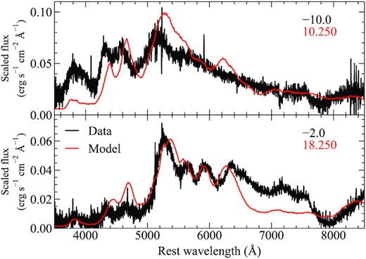
Comparison between spectra of SN 2018byg (black) and our model with a 0.9 M⊙ core and a 0.1 M⊙ shell (red). Phases of SN 2018ybq are given relative to r-band maximum, while days since explosion are given for our model. Spectra are shown in scaled flux.
9.3 PTF10ops
PTF10ops was a peculiar SN Ia that showed a light curve significantly broader than that expected for its low luminosity (MB = −17.77 ± 0.04; Maguire et al. 2011). The early light curve of PTF10ops is not well sampled and therefore it is unclear whether it belongs to the group of SNe showing bumps at early times. For this reason, we opt to discuss it separately. Jiang et al. (2018) argued that there was evidence of an early flux excess; however, they stress that this is based on a single point. First detection occurred approximately 17 d before B-band maximum, while the next detection was 6 d later. Making a definitive statement on the origin of PTF10ops is therefore a challenging prospect. Here, we discuss whether PTF10ops is consistent with models of double-detonation explosions.
In Fig. 19, we show a comparison between the light curve of PTF10ops and models with either a 56Ni- or 32S-dominated shell. These models contain a core mass of 0.9 M⊙ and a shell mass of 0.01 M⊙. The mass of 56Ni produced in the core is 0.13 M⊙. For the 56Ni-dominated shell, our model shows a short-lived bump approximately 1 d after explosion that is consistent with the earliest detection of PTF10ops. The lack of detections in the following days and in other bands means that the decline from this initial bump could have simply been missed. This model also provides a good match to the later light-curve evolution, but is slightly too faint in the g band. Conversely, the 32S-dominated model does not match the earliest detection. Again, this model is able to match the light curve towards maximum light, but remains too faint in the g band.
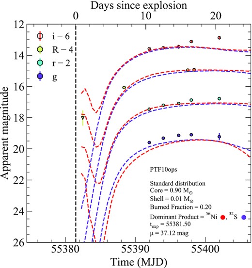
Comparison between the light curve of PTF10ops and our models with a 0.9 M⊙ core, a 0.01 M⊙ shell, and either a 56Ni-dominated (red) or 32S-dominated (purple) composition for the shell. The explosion epoch is shown as a vertical dashed line.
Fig. 20 shows spectra for both models compared to PTF10ops approximately 1 week before maximum light. While both models provide good agreement for wavelengths ≳4500 Å, it is clear that the 56Ni-dominated shell model shows significant line blanketing that is inconsistent with PTF10ops. The 32S-dominated shell model provides improved agreement, although it shows much stronger Ca ii features than those observed.
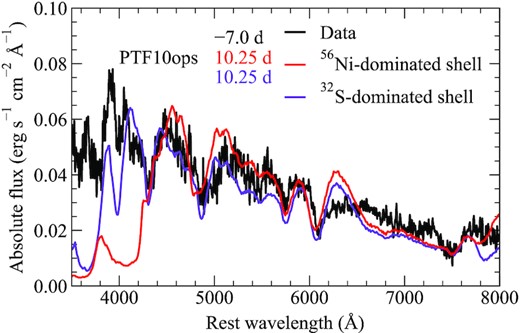
Comparison between the spectrum of PTF10ops approximately 1 week before B-band maximum (black) and our models with a 0.9 M⊙ core, a 0.01 M⊙ shell, and either a 56Ni-dominated (red) or 32S-dominated (purple) composition for the shell. Phases for the model spectra are given as days since explosion. All spectra are shown in an absolute flux scale.
Our models show that if PTF10ops did indeed have an excess of flux at early times, this was not due to a helium shell detonation as its spectra do not show significant line blanketing. Double-detonation models in which the helium shell is dominated by IMEs provide better agreement overall, but they are not able to match the first detection in the light curve. As with normal SNe Ia (Section 8), this could indicate that a somewhat extended 56Ni distribution may be required for these sub-Chandrasekhar-mass models. Alternatively, any early excess emission could be due to interaction, but the lack of nebular spectra and indeed the poorly sampled early light curve makes a definitive conclusion about the nature of PTF10ops a challenging prospect.
9.4 Summary
By comparing our models to observations of SNe Ia with early bumps, we show that a variety of shell masses and compositions are necessary to reproduce the diversity observed. While double-detonation models can match the shapes of the early bumps for all objects (with the exception of iPTF14atg), only those with red colours at maximum light are well matched both photometrically and spectroscopically throughout their evolution following the bump. An investigation of the extent to which double detonations can explain these blue objects requires further observations for a larger sample of objects. We note, however, that all of the currently proposed mechanisms for producing early light-curve bumps appear inconsistent with these blue objects in at least some way. These discrepancies may be due to incorrect colours or lacking features predicted from models of companion and CSM interaction in nebular spectra.
10 CONCLUSIONS
We have presented a large-scale parameter study of the double-detonation explosion scenario. Using the Monte Carlo radiative transfer code presented by Magee et al. (2018), we calculated light curves and spectra for parametrized ejecta structures that were designed to broadly mimic predictions from theoretical explosion models (e.g. Kromer et al. 2010; Polin et al. 2019; Gronow et al. 2020). We considered a range of white dwarf core masses (0.9–1.2 M⊙) and helium shell masses (0.01–0.10 M⊙), which effectively amounts to a range of 56Ni masses. We also considered, for the first time, a large range of possible compositions for the burned material produced in the helium shell, which may result from different levels of pollution in the shell pre-explosion (Shen & Bildsten 2009; Kromer et al. 2010; Waldman et al. 2011; Gronow et al. 2020).
Broadly, our model set may be separated into two categories: those that contain IGEs in the shell and those that do not. Consistent with previous studies (e.g. Jiang et al. 2017; Noebauer et al. 2017; Polin et al. 2019), we find that those models containing IGE in the shell produce a bump in their respective light curves within the days following explosion. The luminosity and time-scale of the bump can show considerable variation, reaching up to MB ∼ −18 and lasting a few days for massive shells. Although the bump is most pronounced for bluer bands (e.g. B), it is also visible at longer wavelengths. At later times, light curves and spectra show extremely red colours and much of the flux below ∼4500 Å has been suppressed. This also leads to fast-declining light curves with rise times to B-band maximum typically around 2 weeks. Conversely, models that do not contain IGE in the shell show a relatively flat and blue colour evolution, and longer rise times that are more typical of normal SNe Ia.
As shown previously (Kromer et al. 2010; Townsley et al. 2019), models that do not contain IGE in the shell provide good agreement with observations of normal SNe Ia around maximum light. Here, we have extended this and shown that the double-detonation scenario is consistent with normal SNe Ia beginning a few days after explosion. Our models do not provide evidence that the helium shell must contain specific elements (e.g. 32S), but rather show that it cannot contain IGE and beyond this requirement the composition has little effect. Therefore, provided the helium shell does not produce IGE during the explosion (which could be due to some amount of pollution), the double-detonation scenario may be considered viable for a range of normal SNe Ia and cannot be excluded. Future explosion models should investigate this further by exploring a range of core and helium shell masses, as well as initial helium shell compositions.
We also compared our models to SNe Ia that show early bumps in their light curves. While we find that the bumps of all objects (with the exception of iPTF14atg) can be reproduced, only those objects with red colours at maximum light (B − V ≳ 1) are matched throughout their evolution. For blue objects, the model spectra at maximum light typically show broader features than observed, in addition to strong flux suppression. Regardless of the composition of the shell, we are unable to simultaneously match the early light curve and maximum light spectra of these blue events. The discovery of additional objects with early light-curve bumps will help us to determine the limit of the double-detonation scenario in reproducing observed light-curve bumps.
Given that our double-detonation models are unable to reproduce the complete evolution of blue SNe Ia showing bumps at early times, this would indicate that an alternative source for the light-curve bumps of these blue objects is necessary. Previous studies have also considered alternative scenarios and generally there is at least some disagreement between these scenarios and the observations. This may be due to either an over- or underprediction of UV flux or the lack of features predicted by companion and CSM interaction scenarios in nebular spectra. It is therefore clear that there is much that remains unknown about the origin of the light-curve bumps in SNe Ia. As current and future facilities, such as the Zwicky Transient Facility and the Vera C. Rubin observatory (Legacy Survey of Space and Time; LSST), discover more SNe Ia within hours of explosion, an investigation of general trends among the class will become possible. This should provide further insights into the nature of these enigmatic bumps.
ACKNOWLEDGEMENTS
We thank the anonymous referee for their detailed and constructive comments, which helped us to improve the clarity of our manuscript. We thank U. Nöbauer and A. Polin for providing densities and compositions for models used in their respective works. This work was supported by the Trinity Centre for High Performance Computing (Research IT, Trinity College Dublin). Calculations were performed on the Kelvin cluster maintained by the Trinity Centre for High Performance Computing. This cluster was funded through grants from the Higher Education Authority, through its Programme for Research in Third-Level Institutions (PRTLI) programme. This work made use of the Queen’s University Belfast High Performance Computing (HPC) Kelvin cluster. MM and KM were funded by the EU/H2020/ERC grant number 758638. This research made use of tardis, a community-developed software package for spectral synthesis in SNe (Kerzendorf & Sim 2014). The development of tardis received support from the Google Summer of Code initiative and from the European Space Agency’s (ESA) Summer of Code in Space programme. tardis makes extensive use of astropy and pyne. This work made use of the Heidelberg Supernova Model Archive (HESMA; https://hesma.h-its.org).
DATA AVAILABILITY
All models presented in this work are available on GitHub.2
Footnotes
REFERENCES
APPENDIX A: START TIME CONVERGENCE TEST
All models presented in this work were calculated assuming a start time of 0.5 d after explosion, which is comparable to the decay time-scale of some of the radioactive isotopes included in the model. For packets injected before the start of the simulation, diffusion relative to the matter in the ejecta is assumed to be negligible. The energy of these packets is also reduced to account for work done on the ejecta (see e.g. Lucy 2005).
In Fig. A1, we show 52Fe-dominated shell models calculated with earlier start times of 0.2 and 0.4 d after explosion, as well as later times of 0.6, 0.8, and 1.0 d after explosion. As demonstrated by Fig. A1, the choice of 0.5 d after explosion does not significantly impact the light curve. From ∼1 d after explosion, all models produce comparable light curves to each other and show only minor variations (≲0.05 mag) consistent with Monte Carlo noise. Assuming a later start time of 0.8 d after explosion does not reproduce the first light-curve point of our nominal 0.5 d case. For earlier start times, however, the light curves show good agreement with our nominal case. Therefore, although the half-life of 52Fe, for example, is shorter than our 0.5 d start time, the light curves in this case do not show significant variation when assuming earlier start times.
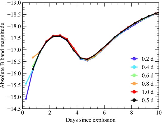
Light curves calculated with different simulation start times for a 52Fe-dominated shell. Our nominal start time of 0.5 d after explosion is shown in black.
APPENDIX B: EFFECTS OF CORE 56Ni MASS
As discussed in Section 3.1, the 56Ni masses of our models are based on those of similar models presented by Kromer et al. (2010) and Polin et al. (2019). Kushnir et al. (2020) present a detailed study of bare, sub-Chandrasekhar-mass detonation models and show that the 56Ni masses presented in these works may be systematically lower than those determined by other studies. Predicted 56Ni masses calculated by Kushnir et al. (2020) are shown in Fig. 3(a) for their default set-up. Also shown are 56Ni masses presented by Shen et al. (2018) for white dwarfs in the range of ∼0.9–1.1 M⊙, which show only minor variations for different metallicities and agree with those of Kushnir et al. (2020).
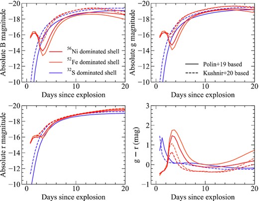
Light curves and colours for models with different core 56Ni masses. All models shown have a 1.0 M⊙ core and a 0.10 M⊙ shell, of which 50 per cent is burned to elements heavier than helium. We show models with dominant shell products of 52Fe and 32S, as representative of models with IGE- and IME-dominated shells.
Fig. B1 shows that the increased 56Ni mass results in brighter B- and g-band peaks by ∼0.35 mag for our 32S-dominated shell model. This model also begins to rise slightly earlier (by ∼0.5 d), although there is not a significant shift in the time of peak brightness (i.e. ≲0.5 d). For our 56Ni- and 52Fe-dominated shell models, the changes from an increased 56Ni mass are more dramatic, particularly in the B band. In these cases, the B-band peaks are brighter by ∼0.6–0.7 mag, while the g-band light curves experience slightly more modest increases of ∼0.4–0.5 mag. Again, these models are brighter at early times, but there is no shift in the time of peak brightness. Although the shapes of the main rising light curves differ due to the increased 56Ni masses, the shapes of the early light-curve bumps are unaffected as these are primarily driven by the material in the shell. The rise time and magnitude of the bump peak are unaffected; however, the decline after the peak of the bump is less pronounced. As the increased 56Ni mass models begin to rise earlier, the difference between the peak of the bump and the minimum after the bump is reduced. This may make bumps less distinguishable in some cases as the earlier rise of the light curve produces more of a ‘shoulder’ in the light curve than a well-defined rise and decline (such as those shown in the r band in Fig. B1).
In Fig. B1, we also show the colour evolution for these models. This is further reflected in Fig. B2, which shows spectra for each model at 3.25, 7.25, and 18.25 d after explosion. For our 32S-dominated shell model, the g − r colour is bluer by ≲0.15 mag throughout its evolution. This model also exhibits slightly higher velocities for the spectral features produced at all epochs. Again, the 56Ni- and 52Fe-dominated shell models show larger changes. At their reddest points (∼4 d after explosion), the higher 56Ni mass models show a shift to bluer g − r colours between ∼0.6 and 0.8 mag, while at their bluest points this shift is ∼0.3–0.4 mag. Therefore, the ‘red bump’ (i.e. the transition a few days after explosion from blue colours to red, and back to blue again) becomes less pronounced and the Δg − r for this transition decreases from ∼1.6–1.7 to ∼1.0–1.4 mag. Interestingly, our 56Ni- and 52Fe-dominated shell models with increased 56Ni masses show a bluer g − r colour than the 32S-dominated shell model between approximately 1 and 2 weeks after explosion. This is somewhat misleading, as Fig. B2 shows that the spectra at these epochs for our 32S-dominated shell model are bluer and this is indeed reflected in the U − B and B − V colours. The appearance of the bluer g − r colours for the 56Ni- and 52Fe-dominated shells is likely due to increased fluorescence emission at these wavelengths. Similar to the 32S-dominated shell model, the increased 56Ni mass also causes a slight shift to higher velocities for spectral features in the case of our 56Ni- and 52Fe-dominated shell models.

Light curves and colours for models with different core 56Ni masses. All models shown have a 1.0 M⊙ core and a 0.10 M⊙ shell, of which 50 per cent is burned to elements heavier than helium. We show models with dominant shell products of 52Fe and 32S, as representative of models with IGE- and IME-dominated shells.
APPENDIX C: EFFECTS OF RELATIVE ISOTOPE ABUNDANCES
In Fig. 4, we show the assumed relative abundances of isotopes in the helium shell for our models. In addition, we also show distributions in which the relative mass fraction of the dominant shell product decreases (broad distribution) or increases (narrow distribution). Here, we discuss how these different distributions affect the light curves and spectra for our models.
As demonstrated in Fig. C1, changes in the relative abundances of isotopes in the helium shell have only minor effects on the light curves. For our 32S-dominated shell models, only a slight change in colour is observed at early times. For the 52Fe-dominated shell models, the effect is most pronounced in the B band at early times. Relative to our standard case, the broad distribution shows a somewhat fainter early bump, which is not surprising given the decrease in mass fraction of radioactive isotopes. At later times, the narrow distribution is brighter than both our standard and broad distributions in the B band. In the narrow distribution, as the mass fraction of 52Fe increases, the relative fractions of all other isotopes decrease. Therefore, that the narrow distribution is brighter at later times likely points to the decreased contribution to line blanketing from having fewer different elements present in the ejecta.
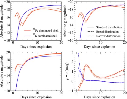
Light curves and colours for models with different shell isotope distributions. All models shown have a 1.0 M⊙ core and a 0.04 M⊙ shell, of which 50 per cent is burned to elements heavier than helium. We show models with dominant shell products of 52Fe and 32S, as representative of models with IGE- and IME-dominated shells.
In Fig. C2, we show how the spectra are affected by changes in the relative abundances of the shell isotopes. Again, it is clear that our 32S-dominated shell model shows only minor changes throughout its spectral evolution. At early times, the effect of a decreased 52Fe fraction is clearly apparent from the fainter and redder spectrum.
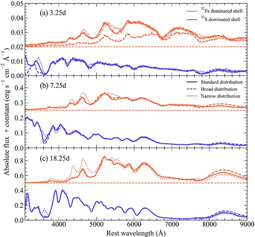
Spectra for models with different shell isotope distributions. All models shown have a 1.0 M⊙ core and a 0.04 M⊙ shell, of which 50 per cent is burned to elements heavier than helium. We show models with dominant shell products of 52Fe and 32S, as representative of models with IGE- and IME-dominated shells. Spectra are shown at three epochs relative to explosion: 3.25, 7.25, and 18.25 d.
