


ABSTRACT
The discovery of optical/UV (ultraviolet) tidal disruption events (TDEs) was surprising. The expectation was that, upon returning to the pericentre, the stellar-debris stream will form a compact disc that will emit soft X-rays. Indeed, the first TDEs were discovered in this energy band. A common explanation for the optical/UV events is that surrounding optically thick matter reprocesses the disc’s X-ray emission and emits it from a large photosphere. If accretion follows the super-Eddington mass infall rate, it would inevitably result in an energetic outflow, providing naturally the reprocessing matter. We describe here a new method to estimate, using the observed luminosity and temperature, the mass and energy of outflows from optical transients. When applying this method to a sample of supernovae, our estimates are consistent with a more detailed hydrodynamic modelling. For the current sample of a few dozen optical TDEs, the observed luminosity and temperature imply outflows that are significantly more massive than typical stellar masses, posing a problem to this common reprocessing picture.
1 INTRODUCTION
A tidal disruption event (TDE) occurs when a star approaches a supermassive black hole (BH) in a galactic centre and reaches the tidal radius where the tidal force is strong enough to overcome the star’s self-gravity. After the disruption, about half of the stellar debris is unbound. The other bound half falls back to the BH with a fallback rate |$\dot{M}_{\rm fb}\propto t^{-5/3}$| (Rees 1988; Phinney 1989). Upon returning to the pericentre, if the fallback stream circularized rapidly it will form a compact accretion disc. A disc of this size will produce soft X-ray/UV (ultraviolet) emissions. About 10 TDEs, whose location is consistent with the centre of their host galaxies and their light curve decays as the accretion rate ∝ t−5/3, have been detected in the soft X-ray band by the ROSAT survey (Brandt, Pounds & Fink 1995; Grupe et al. 1995; Bade, Komossa & Dahlem 1996; Grupe, Thomas & Leighly 1999; Komossa & Bade 1999; Komossa & Greiner 1999; Greiner et al. 2000), XMM–Newton (Esquej et al. 2007, 2008), and Chandra (Maksym et al. 2013; Donato et al. 2014; see Komossa 2015 for a review of these early observations).
A different class of TDEs, hereafter denoted ‘optical TDEs’, was discovered in the last decade in optical and UV bands. Like the earlier X-ray TDEs, these events are also located in galactic nuclear regions and their light curves decline roughly as t−5/3. A few dozen such events have been detected by wide-field high-cadence optical/UV surveys, such as GALEX (Gezari et al. 2006, 2008), SDSS (van Velzen et al. 2011), pan-STARRS (Gezari et al. 2012; Chornock et al. 2014), PTF (Arcavi et al. 2014), iPTF (Blagorodnova et al. 2017, 2019; Hung et al. 2017), and ASASSN (Holoien et al. 2014, 2016a,b). Recently, ZTF almost doubled the sample size (Nicholl et al. 2020; van Velzen et al. 2020a).
Common characteristics of optical TDEs that are most relevant to this work are (Hung et al. 2017; van Velzen et al. 2020a,b) (i) a peak bolometric luminosity |$L\sim 10^{44}\, \rm erg\, s^{-1}$|, (ii) a typical duration longer than |$t \gtrsim 100\, \rm d$|, (iii) a blackbody temperature of |$T\simeq 3\times 10^{4}\, \rm K$| that does not vary much during the observation, (iv) spectra dominated by a blue continuum component. Some events show broad emission lines corresponding to the velocity of |$v\lesssim 10^4\, \rm km\, s^{-1}$| (Arcavi et al. 2014). (v) a total emitted energy |$L t \sim 10^{51}\, \rm erg$| that is much lower than the expected total energy from efficient accretion of a solar mass on to a BH (∼1053 erg) or even from the energy required to circularize the flow on to an accretion disc (∼1052 erg). This is the so-called inverse energy crisis (Piran et al. 2015; Stone & Metzger 2016; Lu & Kumar 2018).
These properties of optical TDEs are inconsistent with the classical picture in which soft X-rays from an accretion disc are expected to dominate the emission. Instead, it was proposed that the emission is reprocessed by surrounding matter. Strubbe & Quataert (2009) and Lodato & Rossi (2011) proposed an outflow launched from small radii (probably a super-Eddington disc wind) radiating away its thermal energy. Later on, others (Metzger & Stone 2016; Roth et al. 2016; Dai et al. 2018; Roth & Kasen 2018; Lu & Bonnerot 2020; Piro & Lu 2020) proposed that an outflow (either a super-Eddington disc wind or the result of shocks in stream–stream or stream–disc collisions) expands, remains optically thick, and reprocesses the ionizing continuum from the inner accretion disc. We denote these as ‘reprocessing-outflow’ models. Since the fallback rate is much larger than the Eddington rate, super-Eddington emission (Loeb & Ulmer 1997; Krolik & Piran 2012) and an outflow from the disc (e.g. Blandford & Begelman 1999) are naturally expected. The expanding material surrounds the system and reprocesses the soft X-rays emitting photons in optical/UV band if thermalization is efficient (Roth et al. 2016; Roth & Kasen 2018). Metzger & Stone (2016) have suggested that the outflow carries out a significant fraction of the infalling mass, reducing the mass accreted by the BH and hence the energy generation rate. Alternatively, the outflow can carry out the excess energy in the form of kinetic energy. This would have resolved the ‘inverse energy crisis’ (Piran et al. 2015; Stone & Metzger 2016; Lu & Kumar 2018).
An alternative model (Piran et al. 2015; Krolik et al. 2016) suggests that the observed optical emission is generated by interactions between the bound stellar debris taking place around the apocentre. This model follows the simulations of Shiokawa et al. (2015) who have shown that the fallback stream passes the pericentre without forming a disc and it collides with the debris near the apocentre. Heated by shocks, the interacting part powers the observed optical emission (see also Svirski, Piran & Krolik 2017; Ryu, Krolik & Piran 2020). In this case, the accretion on to the BH is delayed and is possibly inefficient.
In this work, we focus on the former scenario in which we expect an outflow that is relevant to the reprocessing process. Following recent works by Shen et al. (2015) and Piro & Lu (2020), we analyse the condition within the emitting region and estimate the ejecta mass involved in the optical TDEs. We then impose the condition that this mass cannot exceed the disrupted stellar mass, which is of the order of a solar mass and explore its implications on the reprocessing model. We organize the paper as follows. In Section 2, we develop the method to estimate the ejecta mass of optical transients in a general quasi-spherical optically thick situation using the observed luminosity and temperature. In Section 3, we apply this method to supernovae (SNe) and confirm that we can estimate the ejecta mass with a good accuracy. In Section 4, we calculate the ejecta mass of available optical TDEs by assuming that the emission is powered by spherically expanding wind. We summarize our results and their implications in Section 5.
2 METHOD
We construct a framework to estimate ejecta mass of optical transients assuming that (i) they expand quasi-spherically and (ii) they are optically thick. The observed photons are thermal and diffuse out of the ejecta. In the context of optical TDEs, this situation arises within the ‘reprocessing-outflow’ model. We note that our framework is relevant not only to explosive phenomena like SNe and other transients (Piro & Lu 2020; Uno & Maeda 2020), but also to quasi-steady-state configurations as was discussed in Shen et al. (2015) for the ultraluminous X-ray source M101 X-1.
The system has two different physical situations depending on whether Rd > Rc or Rc > Rd. In the former case, photons are trapped within the ejecta and advected up to Rd. The observed luminosity is given by the diffusion luminosity there. The observed colour temperature is given by the photon temperature at Rd, which is the same as the gas temperature.1 When Rc > Rd, photons diffuse out from Rd but they are still thermally coupled to the gas. The observed colour temperature is determined by the radiation temperature at Rc. Fig. 1 depicts a schematic picture of the system we consider for the cases of Rd > Rc and Rd < Rc.
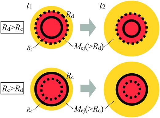
A schematic picture of system at two times t1 < t2 for the two different cases. (Top) Rd > Rc, photons are trapped within the ejecta up to the diffusion radius (Rd, dotted curve) and escape from the regions beyond Rd (marked by yellow colour). (Bottom) Rc > Rd, photons diffuse out of the ejecta beyond Rd, but they are still in thermal equilibrium with the gas up to the colour radius (Rc, solid curve). Outside of Rc (also marked by yellow colour), the photons decouple from the gas. As time progresses, both radii Rd and Rc shrink in the Lagrangian (mass) coordinate. Integrating over time the mass outflow rate |$\dot{M}$| at Rd and Rc, we estimate the ejecta mass that crossed Rd, Mej(>Rd), for the first case and the mass that crossed Rc, Mej(>Rc), for the second.
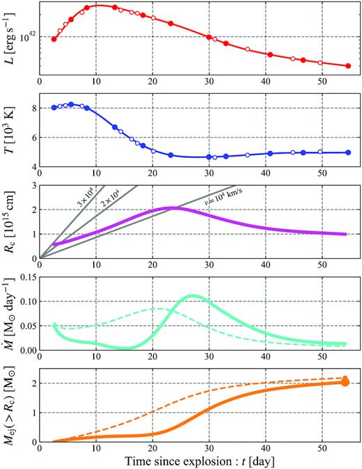
The observed luminosity, temperature, estimated colour radius Rc(> Rd), mass outflow rate, and ejecta mass above the colour radius of SN 2004fe. The observables are taken from fig. 12 in Taddia et al. 2018. In the panel of Rc, the grey lines show the distance of the shells expanding with constant velocities of v = 104, 2 × 10⁴, and |$3\times 10^4\, \rm km\, s^{-1}$|. For |$\dot{M}$| and Mej, we also show the quantities neglecting the term dR/dt (fc = 1) with dashed curves. Including the term dR/dt in equation (3), the mass outflow rate is enhanced (suppressed) before (after) the peak of Rc (|$\simeq 25\, \rm d$|). Note that to obtain smooth fitting curves we used only the solid data points.
3 APPLICATION TO SUPERNOVAE
We apply the method developed in the previous section to a sample of SNe with good data that have been analysed using detailed numerical simulation (Taddia et al. 2018). We compare our results and verify that our method gives a reasonable estimate of the ejecta mass.
We consider a sample of type Ic SNe. For type II SNe, it is well known that the electron scattering opacity decreases drastically due to the hydrogen recombination at the colour radius (e.g. Grassberg, Imshennik & Nadyozhin 1971; Popov 1993; Faran et al. 2019). For type IIb and Ib SNe, most helium recombines shortly after the explosion (|$\lesssim 10\, \rm d$|; Dessart et al. 2011; Piro & Morozova 2014) due to its high recombination temperature. Such an early observation is not always performed and we miss most of the helium ejecta. Thus, in this work, we focus on type Ic SNe for which the ejecta recombination is unimportant and we can ignore the temporal evolution of the electron scattering opacity adopting |$\kappa _{\rm {es}}=0.07\, \rm cm^2\, g^{-1}$| (see e.g. Lyman et al. 2016; Taddia et al. 2018, who estimated the ejecta masses of type Ic SNe using Arnett’s rule). The absorption opacity is dominated by bound–bound transitions because the ejecta are mainly composed of metals (Dessart et al. 2015). Here, we use a constant absorption opacity |$\kappa _{\rm {a}}=0.01\, \rm cm^2\, g^{-1}$| (see Appendix A). Note that when discussing SNe, here, we use a different absorption opacity prescription and opacity values than those used in Section 2.
When the ejecta expand homologously after the explosion (as in the case of SNe), we can simplify further the formula for the outflows. In this case, we can estimate the ejecta velocity at R by v = R/t, where t is the time measured since the explosion. We can then rewrite the mass formula using the observed time instead.
First, we analyse a well-observed SN 2004fe analysed by Taddia et al. (2018). Fig. 2 depicts the time evolution of the bolometric luminosity, colour temperature, calculated colour radius, mass outflow rate at Rc, and ejecta mass out of Rc. For this and the following other SNe, Rc is always larger than Rd (|$t_{\rm crit}\lesssim \, \rm day$|). The mass outflow rate peaks around |$\simeq 25\, \rm d$| that reflects the time evolution of Rc. To see this effect, we also show |$\dot{M}$| and Mej neglecting the term dR/dt (fc = 1) with dashed curves (bottom two panels). When Rc expands (shrinks) with time, |$\dot{M}$| is suppressed (enhanced) from its value with fc = 1 (that ignores this effect). This changes Mej by up to |$\sim 10\, {{\ \rm per\ cent}}$| (bottom panel). In Table 1, we show the resulting ejecta mass and kinetic energy. For a comparison, we also show the ratios of our results (|$M_{\rm ej},\, E_{\rm kin}$|) to the values (|$M_{\rm ej,Hy},\, E_{\rm kin,Hy}$|) obtained by 1D hydrodynamic simulations with flux-limited diffusion (Taddia et al. 2018; see also Bersten, Benvenuto & Hamuy 2011; Bersten et al. 2012 for the details of the calculation). Our results agree with those of the hydrodynamic modelling within a factor of 2. The errors are calculated by considering the uncertainty of the explosion time (other uncertainties such as the luminosity and temperature are not available in the literature and are neglected here).
Ejecta mass and kinetic energy of type Ic SNe estimated by our method (Mej, Ekin). We also show their ratios to those obtained by hydrodynamical modelling (Mej,Hy, Ekin,Hy) by Taddia et al. 2018. Only the uncertainty of the explosion time is included to calculate the errors.
| Event | Mej | Mej/Mej,Hy | Ekin | Ekin/Ekin,Hy |
|---|---|---|---|---|
| (M⊙) | (|$10^{51}\, \rm erg$|) | |||
| SN 2004fe | |$2.0_{-0.3}^{+0.3}$| | |$0.8_{-0.1}^{+0.1}$| | |$1.5_{-0.9}^{+3.4}$| | |$0.8_{-0.4}^{+1.7}$| |
| SN 2004gt | |$1.3_{-0.2}^{+0.2}$| | |$0.4_{-0.1}^{+0.1}$| | |$0.3_{-0.1}^{+0.2}$| | |$0.09_{-0.03}^{+0.1}$| |
| SN 2005aw | |$1.6_{-0.2}^{+0.2}$| | |$0.4_{-0.04}^{+0.1}$| | |$0.6_{-0.2}^{+0.5}$| | |$0.3_{-0.1}^{+0.2}$| |
| SN 2005em | |$2.8_{-0.5}^{+0.5}$| | |$2.6_{-0.4}^{+0.5}$| | |$3.9_{-1.9}^{+4.6}$| | |$15.5_{-7.6}^{+18.2}$| |
| SN 2006ir | |$3.2_{-0.2}^{+0.2}$| | |$0.7_{-0.03}^{+0.04}$| | |$1.2_{-0.3}^{+0.4}$| | |$0.5_{-0.1}^{+0.2}$| |
| SN 2007ag | |$1.5_{0.0}^{+0.3}$| | |$0.6_{0.0}^{+0.1}$| | |$0.9_{0.0}^{+0.6}$| | |$1.5_{0.0}^{+1.1}$| |
| SN 2007hn | |$0.8_{-0.3}^{+0.3}$| | |$0.5_{-0.2}^{+0.2}$| | |$1.6_{-0.9}^{+1.8}$| | |$3.9_{-2.3}^{+4.6}$| |
| SN 2007rz* | |$1.3_{-0.1}^{+0.1}$| | |$0.7_{-0.1}^{+0.1}$| | |$0.6_{-0.2}^{+0.3}$| | |$0.6_{-0.2}^{+0.3}$| |
| SN 2008hh | |$1.9_{-0.3}^{+0.4}$| | |$0.5_{-0.1}^{+0.1}$| | |$1.7_{-0.7}^{+1.5}$| | |$0.6_{-0.2}^{+0.5}$| |
| SN 2009bb | |$2.7_{-0.1}^{+0.1}$| | |$0.6_{-0.02}^{+0.02}$| | |$1.6_{-0.2}^{+0.2}$| | |$0.2_{-0.02}^{+0.03}$| |
| SN 2009dp | |$1.0_{-0.2}^{+0.4}$| | |$0.5_{-0.1}^{+0.2}$| | |$1.3_{-0.7}^{+2.3}$| | |$1.3_{-0.7}^{+2.3}$| |
| SN 2009dt | |$0.4_{-0.1}^{+0.2}$| | |$0.2_{-0.1}^{+0.1}$| | |$0.4_{-0.2}^{+0.5}$| | |$1.0_{-0.5}^{+1.2}$| |
| SN 14gqr* | 0.08 | 0.36 | 0.06 | 0.45 |
We calculate the ejecta mass and kinetic energy of other 11 SNe studied by Taddia et al. (2018)4 and one ultra-stripped envelope SN iPTF14gqr (De et al. 2018). Fig. 3 presents a comparison of our results to those obtained using numerical modelling. Our estimation of ejecta mass (left-hand panel) is consistent with the hydrodynamic calculation while the kinetic energy distribution (middle panel) shows a discrepancy. The right-hand panel depicts a histogram of the ratios of quantities obtained by our estimates to those by numerical modelling. The mean and standard deviation of log (Mej/Mej,Hy) are −0.24 and 0.24, respectively. Thus, our estimation nicely agrees with that by hydrodynamic modelling with an accuracy of a factor of 2. The distribution of log (Ekin/Ekin,Hy) has a mean and standard deviation of −0.11 and 0.56, respectively. This poorer agreement is because the kinetic energy is more sensitive to the estimate of the velocity which in turn depends on the explosion time (see error bars in right-hand panel of Fig. 3).
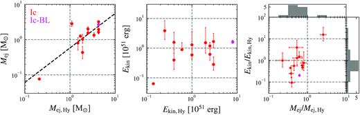
(Left) A comparison of ejecta mass estimated by our method Mej with those obtained by hydrodynamical modelling, Mej,Hy (Taddia et al. 2018). The red and magenta points show the type Ic and broad-line Ic (Ic-BL) SNe, respectively. The black dashed line shows the best fit to the points: log Mej = 0.98log Mej,Hy − 0.24. (Middle) Same as for the left-hand panel but for the kinetic energy. (Right) The distribution of the ratios, Mej/Mej,Hy and Ekin/Ekin,Hy. The mean and standard deviation of the distributions in log space are −0.24 and 0.24 for the mass ratio, and −0.11 and 0.56 for the energy ratio, respectively.
We briefly mention an interesting result of our method concerning the density profile of SN ejecta. Since we estimate the density ρc for each observation time t, we can reconstruct the density profile of the ejecta by correcting the expansion effect ρt3. Fig. 4 depicts a reconstructed density profile of SN 2004fe in the velocity coordinate. The profile could be described by a broken-power-law and it is consistent with the expected structure (Chevalier & Soker 1989; Matzner & McKee 1999). These works show that the power-law indexes of the inner (slow) and outer (fast) parts are ∼−1 and ∼−10, respectively. As shown in Fig. 4, the inner-part’s index of ∼−1.5 agrees with their results, while the outer part has a shallower slope similar to that given by Sakurai (1960), ≃ −5.26.
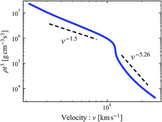
Density profile of SN 2004fe in the velocity coordinate reconstructed by correcting the expansion effect (ρt3). The profile is described by a broken-power-law function consistent with Chevalier & Soker (1989) and Matzner & McKee (1999). The inner part has a slope ρ ∝ v−1.5 and the outer part has a similar power-law index to that expected for Sakurai’s solution: ρ ∝ v−5.26 (Sakurai 1960).
4 EJECTA MASS OF OPTICAL TDES
We turn now to our original goal estimating the ejecta mass of optical TDEs. We focus on the ‘reprocessing-outflow’ model, where we can assume that a quasi-spherical wind is launched and the thermal photons reprocessed by this wind diffuse out from the outflow (Metzger & Stone 2016; Roth et al. 2016; Dai et al. 2018; Roth & Kasen 2018; Lu & Bonnerot 2020; Piro & Lu 2020).
Consider an optical TDE whose luminosity and temperature are known as a function of time. We integrate equations (9) and (14) up to the end of the observation time. We use the electron scattering opacity of |$\kappa _{\rm es}=0.35\, \rm cm^2\, g^{-1}$| and the Kramers’ absorption opacity with κ0 = 4 × 1025 (see Appendix A) assuming that the ejecta’s chemical composition is solar. Different from the homologously expanding SN ejecta, we do not have here a good estimate of the velocity. As the system is quasi-stationary, the outflow may be launched with a constant velocity, we fix the velocity and vary it as a parameter (we will return to this point later). Similarly, we neglect the term of dR/dt in the mass outflow rate, which becomes |$\sim 10^{15-16}{\, \rm cm}/100{\, \rm days}\simeq 10^{3-4}\, \rm {km\, s^{-1}}$| for a typical event. This simplification gives us a conservative estimate of ejecta mass (smaller mass) because the radii Rd and Rc shrink during observations, increasing |$\dot{M}$|.
Fig. 5 depicts the time evolution of the observables (L and T), radius, mass outflow rate, and ejecta mass beyond the radius for ASASSN-14ae, 14li, and 15oi (as Fig. 2) for an assumed fixed velocity of |$v=10^4\, \rm km\, s^{-1}$|. In this case, the diffusion radius is always larger than the colour radius Rd > Rc. The ejecta mass exceeds a solar mass as early as 5–30 d after the discovery.
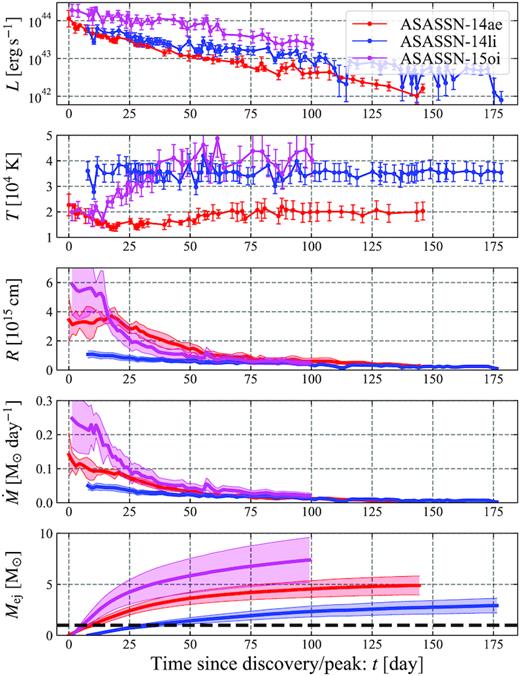
Same as Fig. 2 but for optical TDEs ASASSN-14as (red), 14li (blue), and 15oi (magenta) for a fixed velocity of |$v=10^{4}\, \rm km\, s^{-1}$|. The observables are taken from Holoien et al. (2014, 2016a,b). The shaded regions in the bottom three panels denote the error range calculated when the observational statistical errors in upper two panels are taken into account. The ejecta mass exceeds M⊙ (black dashed line), as early as 5–30 d after the discovery. As noticed by Piro & Lu 2020, Rd is larger than the blackbody radius Rbb ≡ (L/4πσSBT4)1/2, which is commonly used to estimate the size of ejecta (see e.g. Hung et al. 2017). This is not inconsistent because in the situation we consider Rbb has nothing to do with the emission process (see also Nakar & Sari 2010).
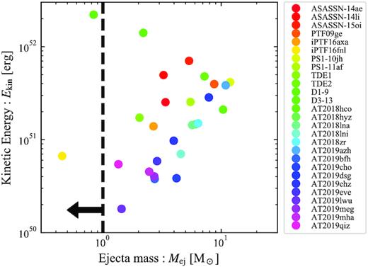
Fig. 6 depicts the ejecta mass of 27 optical TDEs (data are taken from Hung et al. 2017; van Velzen et al. 2020a)5 calculated for different velocities ranging from v = 3 × 10² to |$3\times 10^4\, \rm km\, s^{-1}$|. The estimated ejecta mass peaks at the critical velocity of |$v_{\rm crit}\simeq 10^4\, \rm km\, s^{-1}$| for which Rd = Rc (Note the dependences of the outflow rate, |$\dot{M}\propto v(\propto v^{-1/2})$| for v < vcrit(v > vcrit), see also equation (20) and Shen et al. 2015). Interestingly, this critical velocity is comparable to those suggested by line broadening (Arcavi et al. 2014 but see also Roth et al. 2016; Roth & Kasen 2018 for other mechanism giving the observed line broadening) and expected in the ‘reprocessing-outflow’ model (Metzger & Stone 2016). For most TDEs, the ejecta mass is larger than a solar mass for velocities of |$v\simeq 3\times 10^{3}\!-\!10^4\, \rm km\, s^{-1}$| even in our conservative calculation. The mass is smaller than a solar mass if the ejecta velocity is lower than |$v\lesssim 10^{2-3}\, \rm km\, s^{-1}$|. Such low velocities lower than the escape velocity are unlikely in the system powered by a super-Eddington disc. Moreover, in this case, the ejecta’s kinetic energy is as small as |$E_{\rm kin}\lesssim 10^{49}\, \rm erg$|, and this outflow does not solve the ‘inverse energy crisis’.

Estimated ejecta mass of observed optical TDEs for different ejecta velocities. The grey dashed lines show the kinetic energy at each velocity. As a reference, the black dashed line denotes M⊙. Typical TDE debris should be below this line. For each event, the ejecta mass has a peak at the critical velocity |$v_{\rm crit}\simeq 3\times 10^3\!-\!10^4\, \rm km\, s^{-1}$| (equation 17). When v < vcrit (v > vcrit), the colour radius is larger (smaller) than the diffusion radius, Rd < Rc (Rc < Rd). For the ejecta mass to be sufficiently small, the velocity should be smaller than |$v\sim 10^{2-3}\, \rm km\, s^{-1}$|. The grey shaded regions show velocities excluded by the observations of line widths |$v\lesssim 10^4\, \rm km\, s^{-1}$| or lower than the escape velocity |$v_{\rm esc}\simeq 10^3\, \rm km\, s^{-1}$|.
The ejecta mass and the kinetic energy calculated by setting the velocity to the escape velocity at Rd or Rc, v = vesc(R).
Finally, we comment on the results by Piro & Lu (2020). These authors updated the formalism of Metzger & Stone (2016). Assuming density and temperature profiles, they reproduced a TDE light curve with ejecta mass of |${M}_{\rm {ej}}=0.5\, \mathrm{M}_\odot$|. However, they obtained a luminosity of |$\sim 10^{43}\, \rm erg\, s^{-1}$| and temperature |$\sim 10^{5}\, \rm K$| (see their fig. 5), which are inconsistent with those observed for typical TDEs: |$\sim 10^{44}\, \rm erg\, s^{-1}$| and |$\simeq 3\times 10^4\, \rm K$|. Using such a low luminosity and high temperature, we also obtain an ejecta mass that is less than a solar mass.
5 SUMMARY
We present here a new method, based on earlier ideas of Shen et al. (2015) and Piro & Lu (2020), to estimate the ejecta mass of optical transients that involve a quasi-spherically expanding outflow and have a thermal spectrum. To test the method, we calculated the ejecta mass of type Ic SNe and confirmed that it gives a reasonable estimate with an accuracy of a factor of 2. Interestingly, for a well-observed SN we can also explore the velocity and density structure of the ejecta and we find a density profile consistent with the expected structure (Sakurai 1960; Chevalier & Soker 1989; Matzner & McKee 1999).
Assuming the ‘reprocessing-outflow’ model in which TDEs are powered by a compact source (accretion disc) whose soft X-ray emission is reprocessed at a larger radius to optical/UV emission (Metzger & Stone 2016; Roth et al. 2016; Dai et al. 2018; Roth & Kasen 2018; Lu & Bonnerot 2020; Piro & Lu 2020), we apply this method to optical TDEs. Unlike SNe, the outflow is not expanding homologously and it is in a quasi-steady state. As a result, the velocities are unknown. While observations show line broadening corresponding to |$v\sim 10^4\, \rm km\, s^{-1}$| (e.g. Arcavi et al. 2014), it is not clear that this reflects the outflow velocity (Roth et al. 2016; Roth & Kasen 2018). Hence, we assume different ejecta velocities and explore the dependence of the results on the adopted velocity. As we expect a quasi-steady state outflow, the assumption of a constant velocity is reasonable. Alternatively following hydrodynamic modelling by Shen et al. (2016), we use the escape velocity.
We find reasonable ejecta masses (less than solar) only for ejecta velocities less than about 1000 |$\rm km\, s^{-1}$|. The corresponding ejecta kinetic energy is smaller than |$10^{49}\, \rm erg$|, which is well below the expected value (|$\sim 10^{52-53}\, \rm erg$|) if the ejecta are launched from the compact source and does not resolve the inverse energy crisis. For larger velocities comparable to those inferred from the line width or implied by the escape velocity, |$v\simeq 3\times 10^3\!-\!10^4\, \rm km\, s^{-1}$|, the ejected mass is significantly larger than solar. These results cast some doubt on the overall picture of a wide range of ‘reprocessing-outflow’ model. We find that either the resulting wind would be too massive or if it is not massive it will not carry sufficient energy to provide the missing ‘energy sink’.
Some reprocessing models (Loeb & Ulmer 1997; Coughlin & Begelman 2014; Guillochon, Manukian & Ramirez-Ruiz 2014; Roth et al. 2016) assume a quasi-static layer of poorly circularized debris reprocesses the ionizing continuum from the (efficiently circularized) inner accretion disc. As the assumed velocities are small in this case, the ejecta mass estimates do not pose a problem. However, the ‘inverse energy crisis’ remains here as it is not clear how does the excess energy disappear.
There are several caveats in our results. The first is the assumption of spherical geometry. Clearly, the configuration is not spherical. However, while such deviations are natural in a TDE, we expect that if a deviation is on a large angular scale it could be taken into account by considering the fraction of the solid angle subtended by the outflow. This will not change quantitatively our results. We expect that only large deviations such as a formation of a jet would change our conclusions significantly. van Velzen et al. (2013) use late-time radio observations to put upper limits on Sw J1644 like events (jetted TDEs). They find that at high probability all seven events that they analysed did not have >1052 erg jets. A more detailed analysis would likely yield much stronger limits.
A second caveat is the assumption that the emission is thermalized and is well described by a single temperature blackbody. While this is natural if the emission is indeed reprocessed by optically thick matter, lacking a detailed measurement of the spectrum it is still unclear. Moreover, the temperature is usually determined only by using multiband photometry. If for the given luminosity the true temperature is larger by a factor of 3, the ejecta mass would decrease by a factor of ∼3–10 (see equations 9 and 14), leading possibly to acceptable solution. However, if the luminosity is also varied to reflect the higher temperature, the mass estimate remains valid.
To conclude, we presented here a simple generic method to estimate the outflow from quasi-spherical optical transients. The method is valid for events that are optically thick and when the luminosity and temperature have been measured as a function of time. To test the method, we have applied it to SNe finding an encouraging agreement with more detailed calculations. When applying it to optical TDEs, we find that if indeed the observed emission is thermal and it arises from a compact accretion disc, then the resulting mass of the outflow is too large. This poses a problem for the ‘reprocessing-outflow’ model. This problem does not arise in models in which an outflow is not expected such as the alternative ‘outer shocks’ and in variants of the reprocessing model considering a static envelop. With numerous ongoing and forthcoming observational campaigns aiming at exploring the transient Universe, it will be interesting to analyse in future work other optical transients using this method.
ACKNOWLEDGEMENTS
We thank Iair Arcavi, Chi-Ho Chan, Tamar Faran, Julian Krolik, Keiichi Maeda, Kartick Sarkar, Nicholas Stone, and Masaomi Tanaka for fruitful discussions and helpful comments. We also appreciate an anonymous referee for helpful suggestions. This work was supported in part by JSPS Postdoctoral Fellowship, Kakenhi No. 19J00214 (TM) and by ERC advanced grant ‘TReX’ (TP).
DATA AVAILABILITY
The data underlying this article will be shared on reasonable request to the corresponding author.
Footnotes
Note that beyond Rc the photons and the gas cool adiabatically as T ∝ ρ1/3 and Tg ∝ ρ2/3, respectively. However, Compton heating will heat the gas to the same temperature as the radiation in radiation-pressure-dominated ejecta.
When τeff(Rc) = 1, we have τ(Rc) = (κes/κa)1/2 > 1.
Note that at vcrit, fd = fc.
We exclude SN 2009ca because its luminosity is unusually large among this sample and it might be an outlier.
We exclude AT2018iih that is most likely not a TDE (see Ryu et al. 2020). For example, its luminosity declines much slower than all other TDEs. The corresponding estimated ejecta mass, |$\sim 10^2\, \mathrm{M}_\odot$|, is indeed unreasonably large.
Version 17.01 of the code last described (Ferland et al. 2017).
REFERENCES
APPENDIX A: ABSORPTION OPACITY
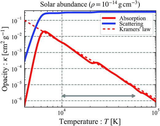
Absorption and scattering opacities for solar abundance ejecta (relevant to TDEs) calculated using cloudy. The absorption opacity is calculated by averaging frequency-dependent continuum (free–free and bound–free) opacity with Planck function (Planck-mean). The dashed line shows the Kramers’ opacity adopted in our calculation, which well approximates the absorption opacity in the TDE temperature range (grey arrow).
For type Ic SN ejecta, bound–bound transitions may dominate the absorption opacity whose dependence on density and temperature is less clear. In analytical light-curve modelling of type Ia SNe, a constant opacity is usually adopted (e.g. Piro & Nakar 2014). Kasen, Badnell & Barnes (2013) present a sample of opacity calculation for silicon, which shows that the opacity does not depend on temperature sensitivity (see their fig. 6). Following the calculation by Dessart et al. (2015, see their fig. 24), we adopt here a constant Planck-mean opacity with |$\kappa _{\rm {a}}=0.01\, \rm cm^2\, g^{-1}$|.
Author notes
JSPS Research Fellow.
