


ABSTRACT
We present observations of a region of the Galactic plane taken during the Early Science Program of the Australian Square Kilometre Array Pathfinder (ASKAP). In this context, we observed the scorpio field at 912 MHz with an uncompleted array consisting of 15 commissioned antennas. The resulting map covers a square region of ∼40 deg2, centred on (l, b) = (343.5°, 0.75°), with a synthesized beam of 24 × 21 arcsec2 and a background rms noise of 150–200 μJy beam−1, increasing to 500–600 μJy beam−1 close to the Galactic plane. A total of 3963 radio sources were detected and characterized in the field using the caesar source finder. We obtained differential source counts in agreement with previously published data after correction for source extraction and characterization uncertainties, estimated from simulated data. The ASKAP positional and flux density scale accuracy were also investigated through comparison with previous surveys (MGPS, NVSS) and additional observations of the scorpio field, carried out with ATCA at 2.1 GHz and 10 arcsec spatial resolution. These allowed us to obtain a measurement of the spectral index for a subset of the catalogued sources and an estimated fraction of (at least) 8 per cent of resolved sources in the reported catalogue. We cross-matched our catalogued sources with different astronomical data bases to search for possible counterparts, finding ∼150 associations to known Galactic objects. Finally, we explored a multiparametric approach for classifying previously unreported Galactic sources based on their radio-infrared colours.
1 INTRODUCTION
The next-generation deep radio continuum surveys, such as the Evolutionary Map of the Universe (EMU) (Norris et al. 2011), planned at the Australian SKA Pathfinder (ASKAP) telescope (Johnston et al. 2008) will open a new era in radio astronomy with potential new discoveries expected in several fields, from Galaxy evolution and characterization to Galactic Science.
In the full-operational mode, the ASKAP telescope is made of 36 12-metre antennas installed in Western Australia, each one equipped with a Phased Array Feed (PAF) receiver (Schinckel et al. 2012), operating with a bandwidth of 288 MHz over the frequency range 700–1800 MHz. The PAF system forms 36 beams and provides an instantaneous field of view of ∼30 deg2, allowing ASKAP to survey the southern sky with unprecedented speed (∼220 deg2 per hour at a target 1σ rms of 100 μJy beam−1) and higher resolution (∼10 arcsec at 950 MHz) compared to existing surveys.
The array has a maximum baseline of 6 km and was completed in mid-2019. During the commissioning phase, the ASKAP EMU early science program (ESP) was launched (2017 October), in which several target fields were observed with the aim of validating the array operations, the observation strategy, and the data reduction pipeline. During this preparatory phase, it became evident that the imaging performance exceeded those of past observations, enabling valid scientific results even with an incomplete array. The scorpio field was the first Galactic field observed during the ASKAP ESP using 15 commissioned antennas (Umana et al., in preparation).
The scorpio survey (Umana et al. 2015) started in 2011 with multiple scientific goals. The original objectives were the study and characterization of different types of Galactic radio sources, with a focus on radio stars and circumstellar regions (e.g. H ii regions). Recently, the study and characterization of stellar relics, such as Galactic supernova remnants (SNRs) in connection with observations at different wavelengths (infrared and gamma-ray primarily) has become an additional target of interest (Ingallinera et al. 2017). The survey also represents an important testbench for the ASKAP data reduction pipeline in the Galactic plane and for the analysis methods designed for the upcoming EMU survey.
This paper is the second of a series of works planned with ASKAP scorpio early science data. In the first paper (Umana et al., in preparation), we discuss the ASKAP’s potential for the discovery of different classes of Galactic objects in comparison with original ATCA observations, and described the data reduction strategies adopted to produce the final mosaic. The goal of this paper is to report a first catalogue of the compact sources present in scorpio. This work will also serve as a validation on real data of the designed source extraction algorithms tested so far with simulated data (Riggi et al. 2016, 2019).
The paper is organized as follows. The ASKAP scorpio radio observations and data reduction are briefly described in Section 2.1. In Section 3 we describe the source extraction methodologies used to build the source catalogue, and discuss the typical performance achieved in source detection and characterization (e.g. completeness, reliability, positional and flux density accuracy). In Section 4 we present the analysis conducted on the resulting source catalogue, from source counts to spectral indices, while in Section 5 we report a comparison with existing astronomical data bases and a preliminary study of unclassified sources. Finally, we report in Section 6 a summary of the results obtained and future prospects.
2 OBSERVATIONAL DATA OF THE SCORPIO FIELD
2.1 ASKAP 912 MHz observations and data reduction
The scorpio field was observed in 2018 January with 15 antennas equipped with the new PAF system version (Mk II) in band 1 (from 792 to 1032 MHz). In this array configuration, the minimum and maximum baselines were respectively 22.4 m and 2.3 km. The former corresponds to a maximum theoretical largest angular scale (LAS) around 50 arcmin at 912 MHz. The total surveyed area covers ∼40 deg2 centred on l = 343.5°, b = 0.75°, extending by a factor of ∼4.8 the area surveyed with past scorpio observations done with the Australian Telescope Compact Array (ATCA) (Umana et al. 2015; Ingallinera et al. 2019).
The calibration and imaging procedures adopted to produce the final mosaic (shown in Fig. 1 and referred to as the scorpio ASKAP map in the rest of the paper) are described in detail in the scorpio paper 1 (Umana et al., in preparation). The green contour in Fig. 1 delimits the field region considered for source extraction (see Section 3), while the yellow contour denotes the scorpio region observed with the ATCA telescope at 2.1 GHz (Umana et al. 2015) (see Section 2.2 for details). The synthesized beam of the final map in J2000 coordinates is 24 × 21 arcsec2 at a position angle of 89°.
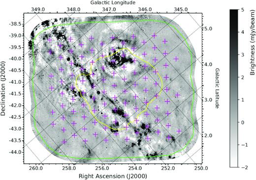
912 MHz mosaic of the scorpio region observed with ASKAP. The purple crosses indicate the beam centre positions for the three interleaved pointings. The green contour delimits the mosaic area considered for source catalogue extraction with the caesar source finder. The yellow contour denotes the scorpio region observed with the ATCA telescope at 2.1 GHz (see the text).
The background level and rms noise were estimated with the caesar finder using parameter values reported in Table A1 (available in the online version of this article). The background rms noise was obtained by interpolating the median absolute deviation (MAD) of pixel fluxes computed over moving sampling boxes of size 10 times the area of the synthesized beam. The background level varies considerably across the surveyed area. In Fig. 2 we report the estimated background noise in μJy beam−1 as a function of the Galactic latitude coordinate b, averaged over the Galactic longitude coordinate l. We observe a noise level ∼200 μJy beam−1 in regions far from the Galactic plane and without bright sources. Close to the Galactic plane, the background noise increases due to the Galactic diffuse emission and the bright emission from extended sources, filling the beam of the telescopes and increasing the system temperature. In regions free of extended sources we observe a background noise around 500–600 μJy beam−1. Only 20 per cent of the field area has a 5σ noise level smaller than 1 mJy beam−1, while for ∼70 per cent of the field the 5σ noise is smaller than 2 mJy beam−1.
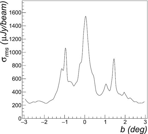
Estimated background noise of scorpio mosaic in μJy beam−1 as a function of the Galactic latitude b and averaged over Galactic longitude l.
2.2 ATCA 2.1 GHz observations and data reduction
The scorpio field was observed with the Australia Telescope Compact Array (ATCA) in the 6A and 6D configurations at the reference frequency of 2.1 GHz, using the 16-cm CABB receiver (observing band from 1.1 to 3.1 GHz) (Wilson et al. 2011). In this array configuration, the theoretical upper limits for the LAS ranges from ∼4.3 to ∼12.2 arcmin. The observations, conducted in different runs from 2011 to 2012, the data reduction strategy, and the scientific results are extensively described elsewhere (Umana et al. 2015; Riggi et al. 2016; Cavallaro et al. 2018; Ingallinera et al. 2019). ATCA observations cover only a small portion of the scorpio field observed with ASKAP, equivalent to 8.4 deg2 (see Fig. 1 for a comparison of the surveyed area size). In Fig. C1 (available in the online version of this article) we present the scorpio ATCA mosaic. We refer to this as the scorpio ATCA map. The achieved rms is ∼30–40 μJy beam−1 and the synthesized beam in J2000 coordinates is 9.8 × 5.8 arcsec2 (position angle of −3°).
The ATCA data, obtained with a bandwidth of ∼1.7 GHz, were divided into seven sub-bands (〈ν/GHz〉 = 1.449, 1.681, 1.844, 2.065, 2.337, 2.614, 2.895) and imaging was independently performed on each of them to produce additional mosaics. The 2.895-GHz channel map was not considered as it was significantly affected by noise and imaging artefacts. The remaining sub-band mosaics (1–6) along with the full band mosaic are used throughout the paper as ancillary data to complement the ASKAP catalogue with value-added information, such as the source spectral indices (see Section 4.2), or to estimate the expected fraction of extended sources (see Section 4.1).
2.3 MOST 843 MHz observations
The Molonglo Galactic Plane Survey 2nd Epoch (MGPS-2) (Murphy et al. 2007), carried out with the Molonglo Observatory Synthesis Telescope (MOST) at a frequency of 843 MHz, completely covers the scorpio field observed with ASKAP with a lower spatial resolution (45 × 45 arcsec2 cosec|δ|) and a source detection threshold of ∼10 mJy. 799 MGPS sources fall in the scorpio region. Their position uncertainty is considered better than 1–2 arcsec (Murphy et al. 2007).
2.4 NVSS 1.4 GHz observations
The NRAO VLA Sky Survey (NVSS) (Condon et al. 1998) covers the scorpio region north of DEC = −40° at a frequency of 1.4 GHz with an angular resolution of 45 arcsec. The detection threshold is ∼2.5 mJy. A number of 853 NVSS sources fall in the scorpio region.
2.5 TGSS 150 MHz observations
The TIFR GMRT Sky Survey (TGSS) (Intema et al. 2017) fully covers the scorpio field at the reference frequency of 150 MHz and with an angular resolution of 25 × 25 arcsec2/cos (DEC − 19°) and a median rms noise of 3.5 mJy beam−1. 249 sources from the first alternative data release (ADR) fall in the scorpio region.
2.6 GLEAM 200 MHz observations
The GaLactic and Extragalactic All-sky Murchison Widefield Array (GLEAM) survey (Hurley-Walker et al. 2017) partially covers the scorpio field in (1° ≤ |b| ≤ 10°, 345° < l < 67°) at the reference frequency of 200 MHz (bandwidth 60 MHz) with an angular resolution of ∼2 arcmin and an rms noise of 10–20 mJy beam−1. 51 sources from the GLEAM Galactic plane catalogue (Hurley-Walker et al. 2019) fall in the scorpio region.
2.7 Supplementary surveys
In this work we will also make use of the following infrared surveys for source classification studies (see Section 5.3):
AllWISE (Cutri et al. 2013) of the Wide-field Infrared Survey Explorer (WISE; Wright et al. 2010): The survey is fully covering the scorpio mosaic region with ∼9.3 × 10⁵ sources detected with S/N > 5 in at least one of the four bands at 3.4 |$\ \mu \mathrm{m}$| (W1), 4.6 |$\ \mu \mathrm{m}$| (W2), 12 |$\ \mu \mathrm{m}$| (W3), and 22 |$\ \mu \mathrm{m}$| (W4). The angular resolutions are 6.1, 6.4, 6.5, and 12 arcsec and the 5σ flux sensitivities for point sources are 0.08, 0.11, 1, and 6 mJy, respectively.
GLIMPSE (Galactic Legacy Infrared MidPlane Survey Extraordinaire) 8.0|$\ \mu \mathrm{m}$| surveys (Churchwell et al. 2009) of the Spitzer Space Telescope (Werner et al. 2004): The surveys (GLIMPSE-I and GLIPMSE-3D) are partially covering (∼74 per cent) the scorpio mosaic region with 8.2 × 10⁵ sources detected with S/N > 5. The angular resolution is 2 arcsec and the 5σ flux sensitivity ∼0.4 mJy.
Hi-GAL (Herschel infrared Galactic plane Survey) 70|$\ \mu \mathrm{m}$| survey (Molinari et al. 2016) of the Herschel Space Observatory (Pilbratt et al. 2010): The survey is partially covering (∼50 per cent) the scorpio mosaic region with 5654 sources detected with S/N > 5. The angular resolution is ∼8.5 arcsec and the 1σ flux sensitivity ∼20 MJy sr−1.
3 COMPACT SOURCES IN THE scorpio FIELD
3.1 Source finding
Compact sources were extracted from the scorpio ASKAP map with the caesar source finder (Riggi et al. 2016, 2019) using an iterative flood-fill algorithm in which the detection threshold is initially set to 5σ and the flooding threshold to 2.5σ. At each iteration the background and noise maps are recomputed, excluding the sources found in the previous iteration and the detection threshold is lowered in steps of 0.5σ. Two iterations were used in this work, corresponding to a final 4.5σ seed threshold level. Algorithm parameter values, reported in Table A1 (available in the online version of this article), resulted from a fine-tuning procedure carried out both on the simulated data sample described in Riggi et al. (2019) and on the simulated maps described in Section 3.3.
We detected 5663 islands1 in the map. 5413 of these were selected as compact source candidates and successfully fitted with a mixture of Gaussian components.
To reject imaging artefacts and sources with a poor quality characterization, we applied these selection criteria to the extracted source sample:
Source fit converged with a |$\tilde{\chi }^{2}\lt $|10;
Positive fitted component peak flux;
Fitted component centroid inside the source island and the mosaic boundary region;
Separation between any pair of source components larger than 8 arcsec (or 2 pixels)
After the selection, 4262 source islands and 4813 fitted source components are left in the preliminary catalogue.
These source counts still include spurious sources, mainly due to imaging artefacts and over-deblending of extended/diffuse emission, surviving the selection criteria. To produce the final catalogue we visually inspected the entire field labelling each source component as ‘real’ or ‘spurious’ in case of a clear unambiguous identification. 4144 fitted source components were tagged as ‘real’ in the final catalogue. Taking into account that the selected survey region is 37.7 deg2, a density of ∼110 selected compact sources per square degree is obtained.
In Table 1 we report a summary of the number of sources extracted at different selection stages. Source numbers labelled with ‘SEL + VIS SEL’ refer to the number of sources passing both the selection criteria and the visual selection. The number of detected sources classified per number of fitted components is also reported.
Number of sources extracted from the scorpio ASKAP mosaic at 912 MHz with the caesar finder at different selection stages and per number of fitted components. The no sel column reports the number of sources extracted by the source finder without any quality cuts applied. The sel column reports the number of sources obtained after applying the selection criteria described in the text. The sel + vis sel column reports the number of sources passing both the quality selection and the visual inspection.
| # components | Selection | ||
|---|---|---|---|
| no sel | sel | sel + vis sel | |
| 0 | 250 | 0 | 0 |
| 1 | 4754 | 3857 | 3786 |
| 2 | 440 | 308 | 173 |
| 3 | 131 | 59 | 4 |
| >3 | 88 | 38 | 0 |
| All | 5663 | 4262 | 3963 |
| # components | Selection | ||
|---|---|---|---|
| no sel | sel | sel + vis sel | |
| 0 | 250 | 0 | 0 |
| 1 | 4754 | 3857 | 3786 |
| 2 | 440 | 308 | 173 |
| 3 | 131 | 59 | 4 |
| >3 | 88 | 38 | 0 |
| All | 5663 | 4262 | 3963 |
Using the same procedure and source selection adopted for the ASKAP catalogue, we extracted 2227 sources and 2369 fitted components from the scorpio ATCA mosaics. The source numbers obtained at different selection stages on the full bandwidth map are reported in Table 2.
Number of sources extracted from the Scorpio ATCA mosaic at 2.1 GHz with the caesar finder at different selection stages and per number of fitted components. The no sel column reports the number of sources extracted by the source finder without any quality cuts applied. The sel column reports the number of sources obtained after applying the selection criteria described in the text. The sel + vis sel column reports the number of sources passing both the quality selection and the visual inspection.
| # components | Selection | ||
|---|---|---|---|
| no sel | sel | sel + vis sel | |
| 0 | 146 | 0 | 0 |
| 1 | 3021 | 2104 | 2096 |
| 2 | 465 | 188 | 120 |
| 3 | 158 | 53 | 11 |
| >3 | 102 | 30 | 0 |
| All | 3892 | 2375 | 2227 |
| # components | Selection | ||
|---|---|---|---|
| no sel | sel | sel + vis sel | |
| 0 | 146 | 0 | 0 |
| 1 | 3021 | 2104 | 2096 |
| 2 | 465 | 188 | 120 |
| 3 | 158 | 53 | 11 |
| >3 | 102 | 30 | 0 |
| All | 3892 | 2375 | 2227 |
3.2 Source cross-matching
To validate and complement the ASKAP catalogue, we cross-matched it with the ATCA catalogue and with the catalogues of supplementary radio (MGPS, NVSS, TGSS, GLEAM) and infrared (AllWISE, GLIMPSE, Hi-GAL) surveys listed in Section 2.1. A summary of the match results is reported in Table 3 and details are provided in the following sections.
Number of cross-matches found between ASKAP source component catalogue and different radio and infrared surveys. Column 4 reports the total number of sources falling in the scorpio mosaic for each survey catalogue. In the last two rows we summed up the number of sources from different catalogues.
| Surveys | Radius (arcmin) | #matches | Total |
|---|---|---|---|
| ATCA | 24 | 648 | 2369 |
| MGPS | 45 | 546 | 799 |
| NVSS | 45 | 189 | 853 |
| TGSS | 24 | 192 | 249 |
| GLEAM | 45 | 32 | 51 |
| AllWISE | 8 | 384 | 123 374 |
| AllWISE + GLIMPSE | 8 | 225 | –* |
| AllWISE + GLIMPSE + Hi-GAL | 8 | 41 | –† |
Notes. *GLIMPSE catalogue has 820 112 sources in scorpio.
†Hi-GAL catalogue has 5654 sources in scorpio.
3.2.1 Cross-matching with ATCA source catalogue
731 ASKAP source components (out of 856 components in the catalogue falling in the ATCA mosaic region) match with at least one source component from the ATCA catalogue within a search radius of 24 arcsec. We visually inspected each cross-match rejecting spurious and unclear associations, e.g. cases in which the ASKAP source flux density measurement is potentially affected by close background sources visible in the ATCA map but not in ASKAP. We finally selected 648 matches. The majority are one-to-one matches (596), while the remaining (52) are one-to-many matches (up to three components). The number of matches purely arising by chance was estimated by averaging the number of matches found between ASKAP catalogue and multiple random ATCA catalogues in which the measured source positions were uniformly randomized inside the ATCA mosaic. With this procedure we found 3.8 ± 0.3 matches between both catalogues. We thus concluded that ∼99.5 per cent of the matches found are likely to be real.
3.2.2 Cross-matching with supplementary radio surveys
We found 688 MGPS sources potentially associated to ASKAP sources within a match radius of 45 arcsec. 546 of them were finally selected for further analysis after excluding multimatches and sources with potentially unreliable flux densities, e.g. affected by imaging artefacts or closely located to very extended sources.
Within a match radius of 45 arcsec we found 226 NVSS sources matching to one or more ASKAP source components. 189 single matches were finally selected after a visual inspection.
192 out of 217 TGSS source matches can be associated to a single ASKAP source within a match radius of 24 arcsec. Similarly, 32 out of 40 GLEAM source matches found within a radius of 45 arcsec were selected for further analysis after excluding multimatches or ambiguous associations.
3.2.3 Cross-matching with supplementary infrared surveys
For the cross-match we considered the AllWISE survey as the primary data set reference due to its full coverage. To limit the number of spurious associations, we selected sources with S/N > 5 in both the W3 and W4 bands with a fraction of saturated pixels smaller than 10 per cent, reducing the number of sources within the ASKAP field to ∼1.2 × 10⁵. A cross-match with ASKAP source catalogue using a match radius equal to the ASKAP beam size (24 arcsec) yields 1319 matches. About 2900 catalogued sources do not therefore have IR counterparts with fluxes above W3 and W4 detection thresholds. The number of source associations arising by chance, estimated using artificial catalogues with random offsets applied, is however compatible with the number of obtained matches, indicating that the vast majority of the matches are spurious.
Selecting a smaller radius (e.g. 8 arcsec as in the Galactic object search analysis) and requiring flux information in all bands, leads to 384 associations allowing us to reduce the number of potential spurious matches to ∼40 per cent. The number of associations decreases to 225 and 41, respectively if we require triple and quadruple matches with GLIMPSE and Hi-GAL catalogues.
The impact of the 5σ limits requested in W3 and W4 bands was investigated on the star/galaxy/quasar data set provided by Clarke et al. (2020).2 The magnitude selection cuts W3 < 11.32 and W4 < 8.03 were found to remove a very large fraction (∼98 per cent) of extragalactic sources from the sample but, unfortunately, also potential radio stars. We thus expect the unmatched sources to be mostly extragalactic, with a smaller percentage of ‘IR-quiet’ (e.g. pulsars) or faint mid-infrared Galactic objects.
3.3 Catalogue selection effects and uncertainties
To evaluate the expected source extraction and characterization accuracy of the produced catalogue, we made use of both simulated data and cross-matches found with other surveys.
Simulated samples were drawn from the scorpio mosaics (both ASKAP and ATCA) using the following approach.4 First, a residual map was obtained by subtracting all compact sources down to a very low detection threshold (2σ). Imaging artefacts, extended and diffuse sources were not removed. A sample of 50 simulated maps was then generated by artificially adding uniformly spaced point sources to the residual mosaic, with a density of 100 deg−2 and exponential flux density distribution (∝ e−λS with λ = 1.6, as for real data above the detection threshold). caesar was finally run on the simulated maps and the same set of quality criteria used for the scorpio mosaics were applied to the simulated catalogue. Source extraction and characterization metrics were estimated by cross-matching injected sources with extracted sources.
3.3.1 Completeness and reliability
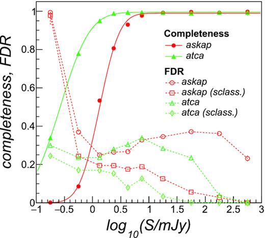
Completeness (filled markers) and false detection rate (FDR) (open markers) as a function of the injected and measured source flux density, respectively, obtained on the simulated ASKAP (red markers) and ATCA (green markers) source catalogues. The solid lines represent the fitted completeness model of equation (1). The open squares and diamonds (labelled as ‘sclass’) represent the false detection rate obtained after applying a neural network classifier, trained to identify spurious fit components in the catalogue.
The false detection rate, reported in Fig. 3 with open dots (ASKAP) and open triangles (ATCA), is found to be of the order of 20–30 per cent, slightly decreasing by a few per cent when moving away from the Galactic plane. False detections are largely due to sidelobes around bright sources (compact or extended) and overdeblending of extended sources. Reliability can be improved by ∼10 per cent after applying a neural network classifier previously trained to identify ‘good’ sources from the data (see Riggi et al. 2019 for more details). Results are shown in Fig. 3 with open squares (ASKAP) and open diamonds (ATCA). To further reduce the false detection rate to acceptable levels (below 1 per cent) we visually inspected the produced catalogue removing spurious sources that were not identified in the automated procedure (see Section 3.1).
For the future we expect this can be substantially improved in multiple ways, e.g. increasing the number of classifier parameters, tuning of classifier hyperparameters, introducing specialized classifiers trained to identify imaging artefacts (e.g. around bright sources) which cannot be efficiently removed with the classifier adopted in this work.
3.3.2 Source position accuracy
Calibration uncertainties σcal can be inferred from the position spread observed in bright sources with respect to a reference catalogue. The Radio Fundamental Catalogue (RFC, version rfc_2020b),6 for instance, contains ∼17 000 radio sources measured in multiple VLBI observations with milliarcsecond accuracy. 5 RFC sources, detected in the X band, cross-match with ASKAP bright sources (four with S/N >200 and one with S/N >20) and have position uncertainty smaller than 0.02 arcsec. The standard deviations (sα = 0.5 arcsec, sδ = 0.4 arcsec) of the observed position offset provide a first measure of σcal since both RFC and ASKAP fit position uncertainties are negligible at high S/N. Additionally, we inferred ASKAP calibration errors using 344 and 80 sources with S/N > 50 matching to MGPS and NVSS catalogues, respectively. The observed standard deviations (sα = 1.3–1.5 arcsec, sδ = 1.3–1.4 arcsec) suggest a slightly larger calibration uncertainty of σcal, α = 1.0–1.1 arcsec and σcal, δ = 0.8–1.1arcsec, after subtracting (in quadrature) the ASKAP fit errors and the MGPS (∼0.9 arcsec from Murphy et al. 2007) or NVSS (∼1 arcsec from Condon et al. 1998) uncertainties.
As no ATCA-RFC matches were found, to infer calibration errors for ATCA, we considered 38 sources detected with S/N > 50 and matched to MGPS sources. In this case, we did not use NVSS data as no matches were found with ATCA above the considered significance level. From the offset standard deviations (sα = 2.1 arcsec, sδ = 2.5 arcsec), we obtained a calibration uncertainty of σcal, α = 1.9 arcsec and σcal, δ = 2.4 arcsec, after subtracting (in quadrature) the ATCA fit errors and the MGPS uncertainties. Such estimates should be regarded as upper limits if MGPS positional uncertainties are underestimated.
Systematic offsets possibly introduced by the fitting procedure were investigated with simulated data for both ASKAP and ATCA. No bias (e.g. median offsets smaller than 0.04 arcsec) was found and, hence, no corrections were applied to the catalogues.
To assess the absolute positional accuracy of the ASKAP ESP data, we considered the median offsets found with respect to the matched sources in RFC, ATCA, MGPS, and NVSS catalogues. We considered only the ASKAP sources with S/N > 50. From the comparison, we found that the ASKAP Dec offsets are negligible (smaller than 0.05 arcsec), while the ASKAP RA is systematically higher than that of the reference catalogues: 〈α〉 = 1.4 arcsec (RFC), 〈α〉 = 1.4 arcsec (ATCA), 〈α〉 = 1.6 arcsec (NVSS), 〈α〉 = 1.7 arcsec (MGPS).7 The RA offset is consistent as a function of the ASKAP source flux density above S/N > 20 (e.g. varying by ∼0.2 at most from bin to bin) and slightly larger than the total position uncertainties estimated above. The astrometric offset, affecting also other ASKAP Early Science observations, is due to a known bug in the askapsoft software version used to process scorpio ASKAP15 data. Recent analysis carried out on newer observations done with the full ASKAP array and improved versions of the reduction software and calibration procedure, do not report significant astrometric offsets. Indeed, we were not able to detect comparable offsets from the preliminary scorpio ASKAP36 maps. For this analysis, we have decided to account for the observed systematic offset by increasing the calibration uncertainty to 1.5 arcsec.
3.3.3 Source flux density accuracy
To assess the absolute flux density scale reliability, we carried out a comparison of the measured ASKAP source flux densities with those reported in previous catalogues at a nearby frequency, such as the MGPS source catalogue. The correlation between ASKAP (S912) and MGPS (S843) source flux densities is reported in the top panel of Fig. 4. The dashed black line corresponds to a perfect correlation (S912 = S843). The bottom panel represents the median relative flux density difference observed as a function of the MGPS flux density. Error bars correspond to the semi-interquartile range of the data in each bin. If all sources were to have a single power-law spectrum S ∝ να, we would ideally expect to observe a relative difference of (912/843)α −1 between the two catalogues. Expected offsets are shown in Fig. 4 with black dashed and dotted lines for three choices of expected spectral indices: α = −0.7 for extragalactic sources, α = 0 for Galactic sources with thermal-dominated emission and an average α = −0.9 as observed in Section 4.2 or in other radio surveys in the Galactic plane (Cavallaro et al. 2018; Wang et al. 2018). For sources brighter than ∼70 mJy, less affected by possible flux density reconstruction bias on both catalogues, we observe that ASKAP flux densities are on average larger by ∼3 per cent with respect to MGPS fluxes. Provided that the source sample is not completely dominated by Galactic thermal sources, we would infer that ASKAP fluxes are overestimated by 9–10 per cent compared to those expected from a mixed population of sources with an average spectral index of −0.9.
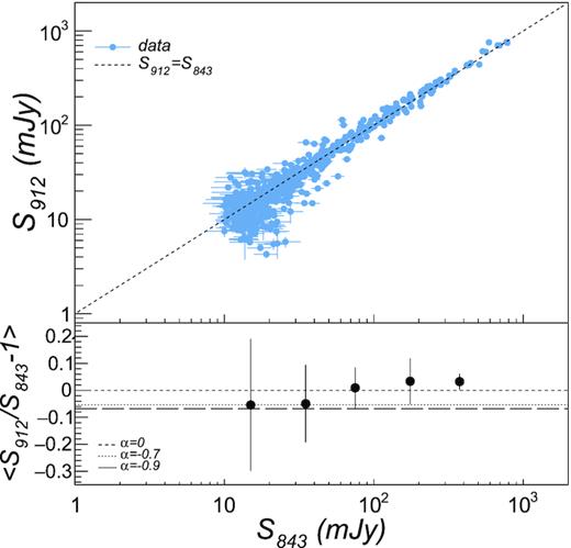
Top: Correlation between flux densities S912 and S843 of cross-matched sources found in ASKAP (912 MHz) and MGPS (843 MHz) catalogues. The dashed black line corresponds to a one-to-one relation (S912 = S843). Bottom: Relative difference between ASKAP and MGPS flux densities. The black dashed and dotted lines represent the difference expected from S ∝ να for three different spectral indices (0, −0.7, −0.9).
We also compared the ASKAP flux densities of selected sources with those expected from a power-law fit obtained with at least four spectral points using MGPS, NVSS, and ATCA data. 45 sources (28 with S/N > 50) are well-modelled by a power law (|$\tilde{\chi }^{2}\lt 2$|, spectral indices ranging from −0.7 to −0.9) over the entire frequency range and, thus, can be used as additional flux calibrators. ASKAP flux densities for these sources were on average found in excess by ∼10 per cent (S/N < 50) and ∼5 per cent (S/N>50) with respect to the predicted values. The standard deviation of the observed offset of bright sources (S/N > 50) is ∼5 per cent and can be used as a measure of σcal. These results suggest a flux density scale inconsistency in the ASKAP data calibration or imaging process that has to be investigated with the full array and improved releases of the data reduction pipeline. The origin of the observed shift is in fact not fully understood at this early stage of ASKAP observations in which the calibration process is not yet optimized. For this reason, we have decided not to correct for it and assume a larger calibration uncertainty (10 per cent) to carry out the analysis described in Section 4. For the ATCA data we have instead assumed σcal = 3 per cent following previous works on the scorpio field (Cavallaro et al. 2018).
4 ANALYSIS
4.1 Estimation of the fraction of resolved sources
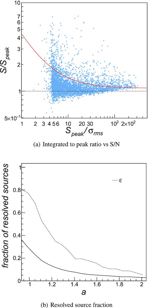
Upper panel: Ratio between integrated S and peak Speak flux densities for catalogued sources as a function of their signal-to-noise ratio S/N. The red line indicates the curve S/Speak = a + |$\frac{b}{S/N}$| (a = 1.08, b = 3.4), used in the XXL survey, above which sources are labelled as resolved. Lower panel: Fraction of catalogued sources that would be classified as resolved as a function of the applied threshold on the parameter a (with b fixed to 3.4), shown with a solid black line. The dashed black line represents the fraction of truly resolved sources ε (found by comparison with ATCA data) that would be classified as resolved as a function of the applied threshold on the parameter a.
Using the scorpio ATCA higher resolution image, it is possible to estimate the number of truly resolved sources at least for a portion of the scorpio field. In Section 3.2.1 we found that 52/648 ASKAP sources match to more than one ATCA source, e.g. ∼8 per cent of the ASKAP catalogued sources have a genuine extended nature. Using this limited source sample, we can compute the fraction of truly resolved sources that would be classified as extended, ε, according to the S/Speak criterion described above. We report the results in Fig. 5(b) with a dashed black line. As can be seen, the S/Speak parameter is not sensitive enough to allow a perfect identification of known resolved sources (e.g. for a = 1.08 we obtained an identification efficiency of ∼60 per cent).
We therefore repeated the analysis including additional parameters. Following Riggi et al. (2019), we considered in particular the ratio E/Ebeam between the source fitted ellipse eccentricity E and the beam ellipse eccentricity Ebeam. We found no significant improvements in the extended source identification capabilities compared to the case of a single discriminant parameter. In light of these results, we will conservatively assume ∼8 per cent as a lower limit in the fraction of extended sources expected in the reported catalogue. Future observations of the scorpio field with the complete array and at higher ASKAP frequencies will provide an improved angular resolution (by a factor of 3–4), enabling a direct identification of additional extended sources over the entire field.
4.2 Spectral indices
Following the convention S ∝ να (where S is the integrated source flux), we estimated the spectral index α of ASKAP catalogued sources using the cross-matches found in Section 3.2 with the ATCA (including also sub-band data), MGPS, and NVSS source catalogues. The number of ASKAP sources detected at one or multiple radio frequencies are reported in Table 4. More than 70 per cent of the sources do not cross-match with any of the considered catalogues and thus no spectral index information can be reported for them. 12 per cent of the sources have flux information only at two frequencies. For them only a two-point spectral index can be reported. These are to be considered as first-order estimates and might not represent a good estimate particularly for sources in which a turnover is present between the two frequencies. For example this is the case for some of the Gigahertz Peaked Spectrum (GPS) and Compact Steep Spectrum (CSS) radio sources (about 40, or ∼20 per cent, in the compilation presented in Jeyakumar 2016). For spectral indices obtained only from ASKAP and ATCA data, taking into account the source extraction performance in both catalogues, we expect to obtain an unbiased estimate of α above 10 mJy at 912 MHz with uncertainties smaller than ∼0.2.
Number of ASKAP sources detected at one or multiple radio frequencies after cross-matching them with MGPS, ATCA (also including sub-band data), and NVSS catalogues.
| # frequencies | # sources | percentage (per cent) |
|---|---|---|
| 1 | 2986 | 72.1 |
| 2 | 504 | 12.2 |
| > 2 | 654 | 15.8 |
| 3 | 119 | 2.9 |
| 4 | 25 | 0.6 |
| 5 | 52 | 1.3 |
| 6 | 63 | 1.5 |
| 7 | 222 | 5.4 |
| 8 | 152 | 3.7 |
| 9 | 21 | 0.5 |
| # frequencies | # sources | percentage (per cent) |
|---|---|---|
| 1 | 2986 | 72.1 |
| 2 | 504 | 12.2 |
| > 2 | 654 | 15.8 |
| 3 | 119 | 2.9 |
| 4 | 25 | 0.6 |
| 5 | 52 | 1.3 |
| 6 | 63 | 1.5 |
| 7 | 222 | 5.4 |
| 8 | 152 | 3.7 |
| 9 | 21 | 0.5 |
For ∼16 per cent of the sources, we have flux information in at least three different frequencies. These data were fitted with a power-law model to determine the spectral indices. When the fit does not converge or does not pass a minimum quality criterion (|$\tilde{\chi }^{2}$| < 10), e.g. due to the presence of outliers in one or more frequency bands, a robust linear regression is performed excluding data points with larger fit residuals. Without improvement (e.g. the |$\tilde{\chi }^{2}$| of the robust fit is still larger than the quality threshold), the reported source spectral index is finally set to the value found using only two frequencies, ASKAP–ATCA or ASKAP–NVSS (if no ATCA information is available).
In Fig. 6 (upper panel) we report the spectral indices obtained from the radio spectrum fitting procedure (635 sources, blue dots) on available ASKAP–ATCA–NVSS–MGPS matches, and those obtained using only ASKAP–ATCA (49 sources, red squares) and ASKAP–NVSS (96, black triangles) matches. Some sources (∼1 per cent of the sample) have a rather extreme spectral index (α < −3 or α < 2.5). Although there is a chance they are pulsars (α<−3) or hyper-/ultracompact H ii regions with an optically thick free–free emission (α < 2.5), their measured indices are somewhat questionable. We note that the majority of the potentially unreliable indices are indeed obtained from two nearby frequencies (ASKAP–NVSS), for which a change in flux density (e.g. due to errors) of ∼10 per cent would lead to a ∼0.5 variation in the measured spectral index. These spectral indices should therefore be treated with caution and be re-estimated with data at additional frequencies. Five sources, in particular, present a very steep spectrum (α<−3), obtained by fitting ASKAP, MGPS, and NVSS data. Spectral index values are in this case mainly determined by NVSS measurements. From a visual inspection, we were not able to spot possible issues in the ASKAP or MGPS flux estimate, e.g. due to a complex background or imaging artefacts. NVSS data for two sources (J171435-392543, J171448-394756) are instead considerably affected by artefacts and thus the reported flux densities may be not accurate. Future ASKAP scorpio observations, bridging the frequency gap between MGPS and NVSS measurements, will allow us to determine the spectral slope more reliably.
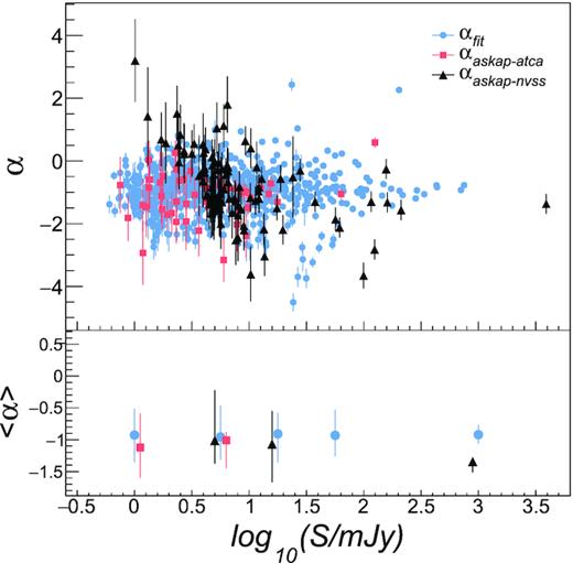
Top panel: Spectral indices of ASKAP 912 MHz source components as a function of ASKAP flux density. The blue dots represent the spectral indices obtained from a power-law fit of available ASKAP–ATCA–NVSS–MGPS data, while the red squares and black triangles indicate the spectral indices obtained from only ASKAP–ATCA and ASKAP–NVSS frequencies, respectively. Bottom panel: Median spectral index for the three samples as a function of ASKAP flux density. Error bars are the interquartile range (IQR) in each flux density bin.
Median spectral indices are reported in the bottom panel of Fig. 6 as a function of the ASKAP source flux density. The median value of fitted spectral indices for brighter sources (<10 mJy) is 〈α〉 = −0.92 (IQR = 0.68). A robust least-squares linear fit to the data of Fig. 6 (top panel) yields similar values. These estimates are consistent within the quoted uncertainties with those obtained in a completely independent analysis (Cavallaro et al. 2018) carried out on a portion of the scorpio ATCA field using only ATCA sub-band data.
4.3 Source counts
In Fig. 7(b) (filled black dots) we report the differential source counts dN/dS (number of sources N per unit area per unit flux density S) obtained by dividing the number of sources found in each flux density bin by the survey area (37.7 deg2 ∼11.5 × 10⁻³ sr) and flux density bin width. Counts were not corrected for expected source detection efficiency and flux density reconstruction accuracy (bias and uncertainty) and were normalized by S−2.5 (the Euclidean slope) (Condon 1984) as conventionally done in other studies of source counts. Error bars denote the statistical Poissonian uncertainties on the obtained counts.
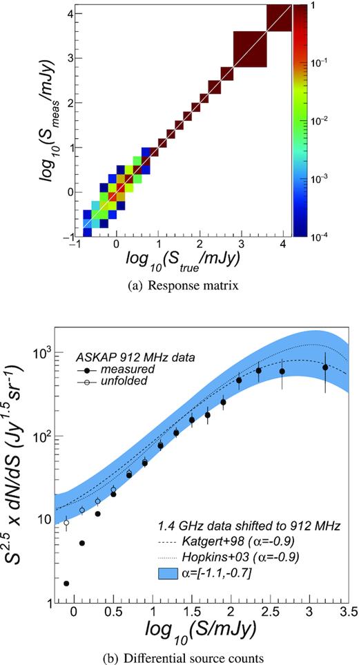
Top: Response matrix used to unfold source detection effects (detection efficiency, flux bias, and uncertainty) from raw source counts. The colour represents the probability rji for a source with true flux density in bin i to be detected with measured flux density in bin j; Bottom: Differential uncorrected source counts of the scorpio survey catalogue normalized to standard Euclidean counts (∝ S−2.5) shown with filled black dots. The open black dots represents the unfolded differential source counts obtained with the procedure described in the text and using the response matrix above. The shaded area represents the existing extragalactic source count data at 1.4 GHz, parametrized by Katgert (1988), Hopkins et al. (2003) and shifted to a frequency of 912 MHz assuming a spectral index α ranging from −1.1 to −0.7 (central value −0.9). Values relative to the median spectral index −0.9 are shown as dashed and dotted lines, respectively.
The resulting matrix values are reported in Fig. 7(a). Above 5 mJy, the correction applied to the source counts is negligible as the catalogue is >98 per cent complete, as shown in Fig. 3, and the flux uncertainty is typically below 1 per cent. Below 5 mJy, the flux uncertainty rapidly increases (up to 30 per cent at 1 mJy) while the completeness rapidly degrades to zero. Source detection inefficiency, thus, causes true counts to be underestimated by a factor ε, while finite flux density uncertainty cause sources to migrate from true to measured flux density bins. As a result, the observed counts in a given bin is contaminated by upward fluctuations from the adjacent lower bins and downward fluctuations from the adjacent upper bins. If the true source counts is steeply falling with flux density, fluctuations from the lower bins dominate and the net effect is an overestimation of the counts.
Resolution bias also causes an underestimation of the true counts. Computed correction factors were found of the order of 5 per cent at 5 mJy and smaller than 1 per cent above 50 mJy.
The unfolded differential source counts, normalized by S−2.5, are reported in Fig. 7(b) with open black dots while numerical values are reported in Table 5. The error bars represent the total uncertainties σtot = |$\sqrt{\sigma _{\text{stat}}^2 + \sigma _{\text{syst}}^2}$| on the unfolded counts, where σstat are the statistical uncertainties, obtained from the Poissonian errors on the uncorrected counts, and σsyst = |$\sqrt{\sigma _{\text{fit}}^2+\sigma _{\text{matrix}}^{2}+\sigma _{\text{cal}}^{2}}$| are the systematic uncertainties. σfit and σmatrix are obtained by propagating the likelihood fit parameter errors and the response matrix uncertainties in the unfolded counts, respectively. Matrix uncertainties have been computed by taking the variance of several response matrices randomized around parametrization errors for ε and σ. Additionally, following Windhorst et al. (1990), a 10 per cent uncertainty is considered in the resolution bias correction εreso. To estimate σcal, we shifted the measured flux densities by ±10 per cent (the calibration uncertainty quoted in Section 3.3.3), repeated the unfolding procedure on the resulting ‘shifted’ spectra and compared the obtained counts with ‘unshifted’ counts.
912 MHz source counts in scorpio field. The columns represent: (1) flux density bin interval ΔS in mJy, (2) flux density bin centre S in mJy, (3) number of catalogued sources N in each flux density bin, (4) corrected number of sources Ncorr, (5) uncorrected normalized differential source counts (S2.5dN/dS), (6) corrected normalized differential source counts (S2.5dN/dS|corr) with statistical (7) and total (8) uncertainties.
| ΔS | S | N | Ncorr | S2.5dN/dS | S2.5dN/dS|corr | σstat | σtot |
|---|---|---|---|---|---|---|---|
| (mJy) | (mJy) | (Jy1.5sr−1) | (Jy1.5sr−1) | ||||
| 0.23 | 0.50 | 111 | 1640.15 | 0.23 | 3.45 | 0.33 | 0.58 |
| 0.37 | 0.79 | 409 | 2183.64 | 1.72 | 9.16 | 0.43 | 1.10 |
| 0.58 | 1.26 | 623 | 1544.04 | 5.22 | 12.93 | 0.50 | 1.47 |
| 0.93 | 2.00 | 700 | 988.56 | 11.69 | 16.51 | 0.56 | 1.83 |
| 1.47 | 3.16 | 600 | 683.18 | 20.00 | 22.77 | 0.87 | 2.59 |
| 2.33 | 5.01 | 507 | 541.79 | 33.72 | 36.03 | 1.55 | 4.22 |
| 3.69 | 7.94 | 354 | 370.61 | 46.97 | 49.17 | 2.51 | 6.07 |
| 5.85 | 12.59 | 287 | 297.43 | 75.98 | 78.74 | 4.46 | 10.09 |
| 9.27 | 19.95 | 204 | 210.18 | 107.76 | 111.03 | 7.82 | 15.67 |
| 14.69 | 31.62 | 146 | 149.81 | 153.88 | 157.89 | 12.48 | 23.68 |
| 23.29 | 50.12 | 84 | 85.92 | 176.65 | 180.68 | 19.50 | 32.96 |
| 36.90 | 79.43 | 60 | 61.22 | 251.76 | 256.89 | 33.38 | 53.75 |
| 58.49 | 125.89 | 55 | 56.02 | 460.46 | 468.98 | 63.84 | 101.74 |
| 157.74 | 223.87 | 46 | 46.77 | 602.18 | 612.27 | 90.02 | 141.26 |
| 314.73 | 446.68 | 16 | 16.25 | 590.32 | 599.37 | 149.02 | 219.10 |
| 3350.11 | 1584.89 | 8 | 8.11 | 657.56 | 666.73 | 241.78 | 348.37 |
Existing source count data at 1.4 GHz, as parametrized by Katgert (1988), Hopkins et al. (2003) and shifted to a frequency of 912 MHz (assuming a spectral index α ranging from −1.1 to −0.7), are shown for comparison as a shaded blue area. The shaded area also accounts for the count fluctuations (∼20 per cent) reported in past works comparing source counts from different extragalactic fields (Windhorst et al. 1990; Hopkins et al. 2003) or from different regions of the same survey (Prandoni et al. 2001; Retana-Montenegro et al. 2018). The observed spread can be due to either systematic uncertainties, different correction factors applied, or to the large scale structure of the Universe (i.e. cosmic variance).
As can be seen, the measured source counts as a function of the source flux density are consistent with the trend reported in other surveys carried out far from the Galactic plane (e.g. see Katgert 1988; Hopkins et al. 2003 and references therein). The discrepancies observed assuming a spectral index α = −0.7, ranging from 15 per cent to 20 per cent, are within the quoted systematic uncertainties. The presence of our Galaxy is also expected to play a role in this comparison. Galactic sources indeed contribute to the overall source counts, although with a smaller fraction (∼5 per cent at least from the analysis presented in Section 5.1). An overdensity effect (∼10–15 per cent), reported for example by Cavallaro et al. (2018), cannot however be clearly identified, being of the same order of the reported uncertainties.
For the sake of completeness we derived the source counts in a region outside the Galactic plane (|b| < 2) following the same procedure described above and using an updated response matrix, parametrized on the considered mosaic region. No significant differences (within few per cent) were found with respect to the source counts obtained over the full mosaic, suggesting that the majority of the unclassified sources have an extragalactic origin.
5 SOURCE CLASSIFICATION
5.1 Search for known Galactic objects
We cross-matched the ASKAP scorpio source catalogue with different astronomical data bases to search for possible associations with known Galactic objects. We restricted the search to the following types of objects:
Stars: associations searched in the SIMBAD Astronomical Data base,11 in the Galactic Wolf–Rayet Star Catalogue12 (Rosslowe & Crowther 2015) and in the Gaia data release 2 catalogue (Brown et al. 2018);
Pulsars: associations searched in the ATNF Pulsar Catalogue13 (Manchester et al. 2005) (version 1.63);
Planetary Nebulae (PNe): associations searched in the Hong Kong/AAO/Strasbourg H-alpha (HASH) Planetary Nebula Data base14 (Parker et al. 2016);
H iiregions: associations searched in the WISE Catalogue of Galactic H ii regions15 (Anderson et al. 2014).
Extended objects, such as the supernova remnants (SNRs) listed in the Galactic SNR catalogue16 by Green (Green 2019), were not considered in this analysis. Possible associations and new detections will be reported in a future work dedicated to scorpio extended sources.
We summarize the cross-match results in Table 6. The number of associations found for each catalogue is reported in column 4 while the expected number of false matches is given in column 5. These were estimated with the same procedure described in Section 3.2, i.e. evaluating the number of matches found within the chosen radius in several ‘randomized’ catalogues. The search radius considered for the matching, reported in column 3, corresponds to the maximum statistical significance of the match signal above the background. The number of objects labelled as ‘confirmed’ in the astronomical data bases is reported in column 6.
Number of sources from different astronomical catalogues (see the text) associated to ASKAP scorpio radio sources.
| Obj. Type | Catalogue | rmatch | nmatches | |$n_{\rm matches}^{\rm random}$| | Confirmed |
|---|---|---|---|---|---|
| (arcmin) | objects | ||||
| Star | SIMBAD | 4 | 20 | 2.3 ± 0.3 | 13 |
| WR Cat. | 4 | 0 | 0 | 0 | |
| GAIA DR2 | 2 | 933 | 874.2 ± 9.6 | 0 | |
| Pulsar | ATNF Cat. | 8 | 21 | 0 | 21 |
| PNe | HASH | 8 | 38 | 0 | 27 |
| H ii regions | WISE | 32 | 67 | 0 | 35 |
| All | – | – | 146* | – | 96 |
Note. * GAIA matches not included in the final count.
Only 146 objects were associated to known classes of Galactic objects, corresponding to ∼4 per cent of the total number of scorpio catalogued sources. The vast majority of the catalogued sources are thus labelled as not classified. A 2D map showing the positions of both classified and unclassified sources is reported in Fig. D1 (available in the online version of this paper).
5.1.1 Stars
Inside the scorpio ASKAP region, we selected 10 628 stars in the SIMBAD data base and 19 Wolf–Rayet stars in the Rosslowe & Crowther (2015) catalogue. These were cross-matched to ASKAP source components within a match radius of 4 arcsec in sky coordinates. Since the GAIA catalogue is densely populated (more than 9 × 10⁶ entries found in the scorpio region) we lowered the search radius to 2 arcsec, comparable to the positional uncertainties obtained in ASKAP. We found 20 associations in SIMBAD, among them 7 YSO (1 confirmed, 6 candidates), and no associations with Wolf–Rayet stars up to a matching radius of 32 arcsec. SIMBAD matches are expected to be real as the estimated number of chance matches is 2.3 ± 0.3 (see Table 6). The associations found with GAIA DR2 (933) are instead dominated by random matches and will not be further considered. A list of the associated objects found is reported in Table E2 (available in the online version of this paper). The reported classification was investigated with infrared and optical data. Details are reported below:
SSTGLMC G343.7018 + 00.0861: invisible in optical and near-IR; clear but not particularly red in the mid-IR. Not immersed in a region of star formation. YSO candidate classification is premature. Could well be extragalactic.
IRAS 16495-4140: likely a YSO. It is a small clump of stars of which two dominate in the near-IR (2MASS). Together they are bright and red in the mid-IR (WISE; not covered by Spitzer).
2MASS J17062471-4156536: classified as a YSO candidate with star-forming activity (and dark cloud) nearby. Could be extragalactic. Invisible in the optical but bright (and red) in 2MASS. Not particularly red in Spitzer and WISE.
SSTGLMC G344.2155-00.7460: only detected in the mid-IR, faintly. There is nothing to suggest otherwise that this is a background AGN. It is not near star-forming complexes and it is next to darker areas of extinction, i.e. viewed through a relatively more transparent region. The YSO classification is questionable.
IRAS 16534-4123: likely extragalactic. It is exceedingly faint in optical and very bright in WISE.
[MHL2007] G345.0052 + 01.8209 1: Class I protocluster. Clump of red stars in 2MASS, no detection in optical, embedded within a diffuse background emission seen with Spitzer (GLIMPSE) and saturating in WISE.
HD 326586: F8 star, bright GALEX (UV) source.
SSTGLMC G342.6544-00.3827: faint, red. Detected in optical and near-IR, not particularly bright or red in mid-IR. Not necessarily a YSO, and no indications that it should be radio-loud. Could well be a background AGN.
IRAS 16472-4401: related by SIMBAD with an IRAS source, undetected in 2MASS. Close to the source’s sky position (≈6 arcsec), a YSO was detected by the ATLASGAL survey at 870 μm (Urquhart et al. 2018).
2MASS J16504054-4328122 (IRAS 16470-4323): while SIMBAD classes it as an AGB star, there is no direct evidence for this. It is strangely yellow in the DECaPS (five-band optical and near-infrared survey of the southern Galactic plane with the Dark Energy Camera (DECam) at Cerro Tololo), unlike any other object around it. It is red in 2MASS but again yellow in Spitzer and WISE. The GAIA data are marginal, so we cannot completely exclude an extragalactic nature.
HD 326392: classified as B8 star ≈830 pc far (Brown et al. 2018). At the stellar distance, the measured flux of HD 326392 corresponds to a radio luminosity of ≈6 × 10¹⁷ ergs s−1 Hz−1, more than one order of magnitude higher than CU Vir (≈3 × 10¹⁶ ergs s−1 Hz−1; Leto et al. 2006), a magnetic late B type star well studied at radio regime. The radio luminosity of HD 326392 is instead more comparable to those of strong magnetic stars of B2 spectral type, level ≈10 kG and luminosity close to 1018 ergs s−1 Hz−1 (Leto et al. 2017, 2018). This suggests HD 326392 as a possible strong magnetic star.
2MASS J17122205-4230414: fairly red but not too faint in the optical, bright in the mid-IR. As such it is isolated, the post-AGB classification seems more likely than a YSO (as listed in SIMBAD). It is found to be slightly extended and classified as a planetary nebula by Suarez et al. (2006) with high confidence, though their optical spectrum shows no trace of [O iii].
TYC 7872-1355-1: Anonymous star, but in a reflection nebula.
MSX6C G346.4809 + 00.1320: YSO, Class 0 (invisible in near-IR) with a 6.7-GHz methanol maser detection by Gaylard & MacLeod (1993) and a single 100 per cent polarized 1665-MHz OH maser peak by Caswell & Haynes (1983).
2MASS J17074166-4031240: likely a YSO. It is invisible in the optical but clear and red in 2MASS; however, the mid-IR emission comes mainly from the bright rim (photodissociation region) of a cloud/H ii region immediately to its side, most likely the origin of the radio emission.
CD-38 11343: Classified as ‘double star’ (er* (M3Ve + M4Ve)) in SIMBAD. Eruptive pair of M dwarfs at 15 pc, with likely expected variability also in radio.
IRAS 17056-3930: very faint red optical, but bright(ish) red near-IR and mid-IR source. However, it is very isolated, there is nothing like it within at least 5 arcmin radius in a field of stars with the nearest sign of star formation activity about 8 arcmin away. Further investigations are needed to address its nature.
IRAS 17056-3916: no detection in optical or near-IR, but very red mid-IR source; possibly unresolved. It is located right at the edge of a dark cloud, which could suggest it is a YSO or explain why it is not seen in the optical. Further investigations are needed to confirm if of extragalactic origin.
Cl* NGC 6318 PCA 7229: Classified as ‘star in cluster’ in SIMBAD. This might in fact be the AGAL G347.919-00.762 YSO, detected in Spitzer data.
TYC 7873-953-1: radio source generically classified by the SIMBAD data base as star. This is associated with a visible source about 1.2 kpc far (Brown et al. 2018). Further, this was discovered as a variable radio source at 1.4 GHz from NVSS data (Ofek & Frail 2011).
We compared the matches found with those obtained in pilot observations of the scorpio field with ATCA at 2.1 GHz. Only 2 of the 10 star associations reported in Umana et al. (2015) are retrieved also in the ASKAP map. Due to a lack of sensitivity, no radio sources are detected in the direction of the two Wolf–Rayet stars (HD 151932, HD 152270) previously detected in ATCA.
For six associated objects, shown in Fig. 8 and reported as top entries in Table E2, we were able to derive a spectral index measurement (column 14) using scorpio ASKAP and ATCA, MGPS, and NVSS data (see Section 4.2). Among them we have four Young Stellar Object (YSO) candidates with fitted spectral index α: 0.21 ± 0.06 (SSTGLMC G343.7018 + 00.0861), 0.02 ± 0.15 (2MASS J17062471-4156536), 0.17 ± 0.09 (SSTGLMC G344.2155-00.7460), 0.43 ± 0.08 ([MHL2007] G345.0052 + 01.8209 1). Taking into account the reported uncertainties, these values are generally consistent with the spectral indices expected in optically thin free–free emission processes from ionized gas. According to Scaife (2012), Ainsworth et al. (2012), Anglada et al. (2018), the free–free radio emission at centimetre wavelengths is ascribed to outflow processes (e.g. thermal jets) causing the required gas ionization, particularly in the earliest protostellar stages (Class 0 and Class I). The resulting YSO radio spectral indices α are expected in the range −0.1<α<1.1 but their values depend on the protostar evolution. For example in collimated outflows, typical of early protostar stages, a radio spectral index α ∼0.25 is favoured, while, for standard conical jets, spectral indices around 0.6 are expected (Reynolds 1986; Anglada et al. 1998). Existing measurements mostly fall in the above range although in some cases the observed spectral indices (<−0.5) suggest a contribution from non-thermal processes (Ainsworth et al. 2012). Our spectral index measurements are found within the range expected from free–free emission. Additional radio data at different frequencies are however needed to further constrain the dominant emission mechanism.
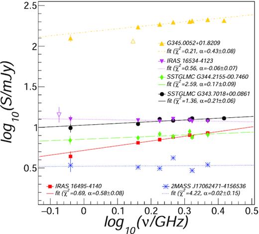
Spectral data of scorpio sources associated to stars in the SIMBAD data base, obtained using ASKAP and ATCA data (filled markers) and previous MGPS and NVSS observations (open markers). The power-law fits are reported with coloured lines.
5.1.2 Pulsars
The ATNF Pulsar data base has 58 catalogued pulsars inside the scorpio region. We carried out a search for possible associations with scorpio source components, finding 21 associations within a matching radius of 8 arcsec and a number of chance matches compatible with zero.
In Table E3 (available in the online version of this paper) we report the full list of matched objects. Four of these (J1654-4140, B1703-40, J1702-4128, J1702-4217), shown as top entries in the table, have spectral index information (column 14) that can be obtained from ASKAP and ATCA data only. Column 12 represents the spectral index reported in the ATNF catalogue from measurements at 0.8, 1.4, and 3.0 GHz (Johnston et al. 1992; Kramer et al. 2003; Jankowski et al. 2018, 2019; Johnston & Kerr 2018). Flux density measurements, available in the literature for three of them (J1654-4140, B1703-40, J1702-4128), are reported in Fig. 9 with open markers. New measurements, obtained in this work, are shown with filled markers. Both ASKAP and ATCA fluxes compare well to existing data, allowing us to derive a new spectral index measurement for all three pulsars. Fit results are shown in the figure with solid, dashed, and dotted lines. The steep spectral index values found for J1654-4140 and B1703-40, reported in Table E3 (column 14), are compatible with the distribution of pulsar spectral indices compiled in Maron et al. (2000) (〈α〉 = −1.8 ± 0.2). The flat spectrum of J1702-4128, confirmed by our ASKAP and ATCA observations, supports the hypothesis of a pulsar wind nebula (PWN) as the origin of the radio emission. This was investigated by Chang et al. (2008) to explain the nature of the X-ray emission from Chandra CXOU J170252.4-412848 but no conclusive evidence was reached. Future ASKAP EMU and POSSUM data might give further evidence for a PWN if this source is linearly polarized.
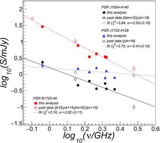
Spectral data for J1654-4140 (open black dots), B1703-40 (open red squares), and J1702-4128 (open blue triangles) pulsars reported in the ATNF pulsar catalogue: kbm + 03 (Kramer et al. 2003), jvk + 18 (Jankowski et al. 2018), jk18 (Johnston & Kerr 2018), jlm + 92 (Johnston et al. 1992), jbv + 19 (Jankowski et al. 2019). ASKAP and ATCA spectral data obtained in this work are shown with filled markers. Single power-law fits are reported with solid, dashed, and dotted lines for the three sample pulsars.
5.1.3 Planetary nebulae
Within our surveyed area, HASH has 60 PNe17 that were cross-matched to ASKAP catalogued sources at different matching radii. A number of 38 associations were found assuming a radius of 8 arcsec. 27 of the 38 matches correspond to confirmed PN objects. The number of chance matches found is compatible with zero. We visually inspected the five confirmed PNe (MPA J1715-3903, MPA J1717-3945, MPA J1654-3845, MPA J1644-4002, PHR J1709-3931) that were not cross-matched to any ASKAP source. In the direction of the first four PNe there are no radio sources in the map. A faint radio source is instead found in the direction of PHR J1709-3931 but it is detected at an S/N of only 4.1.
A full list of associated PNe is reported in Table E4 (available in the online version of this paper). With ASKAP we detected the nine HASH PNe studied with ATCA 2.1 GHz observation in Ingallinera et al. (2019). ATCA flux measurement is however reported in this study for only five PNe (1 confirmed: IRAS 16515-4050, 4 candidates: MPA J1654-4041, PHR J1654-4143, Pre 11, DGPK 2), shown in Fig. 10 and listed as top entries in Table E4. Four PNe were fitted with simple power-law models (labelled as ‘PL’ in Fig. 10) as their radio spectra do not show evidence of spectral curvature in the studied frequency range. Although the fit models are not highly statistically significant, the results constitute a first measurement of the average spectral index for these objects as no other measurements are available in the literature.
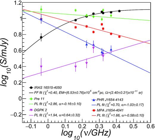
Radio continuum spectra for five PNe obtained using ASKAP and ATCA observations.
For the rest of catalogued PNe we were able to estimate the spectral index by combining our measurements with existing ones at 843 MHz (Murphy et al. 2007) (MOST), 1.4 GHz (Condon et al. 1998; Condon & Kaplan 1998) (VLA), 4.8 GHz (van de Steene & Pottasch 1993) (ATCA). Some of them, obtained using 843 and 912 MHz measurements only, are clearly unreliable due to the limitations discussed in Section 3.3.3.
The spectral indices obtained with data at higher frequencies are found in general agreement with the expected nature of the emission in PNe, i.e. thermal free–free radiation due to electron–ion interactions in the nebula shell (Kwok 2000). The expected spectral indices, however, vary considerably depending on the thermal and electron density scenario, roughly ∼−0.1 in an optically thin regime and positive up to ∼2 (Pottasch 1984) for optically thick PNe. The first scenario is likely in place in MPA J1654-4041, PHR J1654-4143, Pre 11, Vd 1-5, and Vd 1-6 for which we observed negative spectral indices. The second scenario seems favoured for some other detected PNe, e.g. IRAS 16515-4050, DGPK 2, PM 1-119, and PM 1-131. Due to the limited number of radio observations available, the precision achieved on the spectral indices does not allow us to constrain the PN nature and corresponding emission mechanism. Deeper analysis, possibly in combination with IR data as in Fragkou et al. (2018), Ingallinera et al. (2019), will be therefore performed in the future once new ASKAP observations with different frequency bands become available.
5.1.4 H ii regions
Within the scorpio region used for source finding, we found 356 Galactic H ii regions catalogued in Anderson et al. (2014).19 256 of these were classified by these authors as ‘known’ (i.e. objects confirmed by Anderson et al. 2014 or in previous studies, including radio quiet H ii regions), with the rest as candidates (including those closely located to a known H ii region). Their sizes range from 0.2 arcsec to ∼23 arcmin with a median of ∼1 arcmin. Within a matching radius of 32 arcsec we found 67 H ii regions associations.20 The matched H ii regions have a reported radius between 12 and 100 arcsec (average radius ∼52 arcsec). From a visual inspection, we were able to confirm ∼90 per cent of the matches found in the automated analysis.
Thirteen H ii regions were detected in both the ASKAP and ATCA maps. We were able to determine a first measurement of the radio spectral index for 9 of them (6 confirmed objects and 3 candidates). The remaining ATCA sources have either an unreliable spectral fit, due to noisy sub-band data, or an unclear association with ASKAP data. For instance, ASKAP source associated to G344.993-00.265 is located close to another, more compact, H ii region (G344.989-00.269). The higher resolution of ATCA observations allows us to distinguish the two sources when estimating their flux densities. This is not the case for ASKAP data in which the two sources are blended. Future ASKAP observations will provide the required sensitivity, resolution, and additional spectral data to refine and extend this analysis. Finally, an additional spectral index measurement was obtained for G347.921-00.763 using MGPS and NVSS data. More details for each source are reported in Table E5 (available in the online version of this paper).
5.2 Extragalactic sources
A large number of the extracted sources (∼3800 source islands, >95 per cent of the catalogue) are not classified or associated to a known astrophysical object. Following the findings reported in previous radio surveys carried out in the Galactic plane (Cavallaro et al. 2018; Wang et al. 2018) and the comparison with extragalactic source counts reported in Section 4.3, we may reasonably expect that the majority of them are extragalactic objects. A search in the NASA/IPAC Extragalactic Database (NED)21 returned only 20 known objects classified as galaxies (G). Two of them (2MASS J17172771-4306573, 2MASX J16463421-3903086) are found associated to scorpio catalogued sources. Another one (2MASS J17162433-4225102) is likely associated to a faint non-catalogued ASKAP radio source (S/N = 3.7). For the rest, there are no indications for a cospatial radio emission at the current map sensitivity.
We report here a preliminary analysis to increase the number of classified sources and provide the basis for more advanced studies to be done in the future. Indeed some of the unclassified source islands are found to have a bipolar morphology resembling those of radio galaxy lobes or can be visually associated to neighbour islands connected by a radio jet-like emission. We can therefore visually inspect the ASKAP map to search for this kind of object and label them as candidate radio galaxy. Since a precise identification using morphological considerations only is currently severely limited by the resolution of our ASKAP map, we also considered the ATCA map which provided the needed resolution to address some of the unclear identifications. Results are reported in Table 7.
Number of radio galaxies identified in the scorpio ASKAP mosaic per number of islands and labelled according to the degree of confidence reached in the identification (see the text).
| # islands | Degree of confidence | |
|---|---|---|
| low | high | |
| 1 | 103 | 131 |
| 2 | 10 | 28 |
| 3 | 0 | 5 |
| All | 113 | 164 |
| # islands | Degree of confidence | |
|---|---|---|
| low | high | |
| 1 | 103 | 131 |
| 2 | 10 | 28 |
| 3 | 0 | 5 |
| All | 113 | 164 |
A number of 277 candidate radio galaxies were identified. None of them are associated to known NED extragalactic objects. The majority was found associated to one island detected in the catalogue (e.g. other components are either not visible or below the detection threshold) and only a few associated to two or three islands (which may correspond to a single source). The number of source islands associated to the candidate galaxy do not always have a 1-to-1 correspondence to the physical components (e.g. core, lobes). In many cases the latter are in fact visible inside a single island.
For almost half of the cases there were no strong indications whether the radio morphology would suggest a radio galaxy. These have been labelled as candidates with lower degree of confidence in Table 7. About 70 radio galaxy candidates, lying north of Dec = −40 deg, were visually inspected in the QuickLook data release of the VLASS 2–4 GHz survey (Lacy et al. 2020). Only two of them (one is reported in Fig. 11) were firmly confirmed as radio galaxies from their morphology, while the rest are resolved out or only showing the core component. Given the resolution limitations already discussed, future ASKAP observations at higher resolution will be needed to confirm the nature of these candidates.

A sample radio galaxy classified with high-confidence in both the ASKAP scorpio map (colour scale and solid black contour) and in the VLASS survey (superimposed solid green contours). The ellipse at the bottom left indicates the ASKAP synthesized beam size.
Spectral information, measured only for 74 source components found in candidate radio galaxy islands, may provide additional hints for these studies, at least for a subset of the sources. Following the classification scheme reported in Zajaček et al. (2019), 62 of them have a lobe-like steep index (α < −0.7), 6 are found with a jet-like index (−0.7 ≤ α ≤ −0.4) and 6 with a flatter core-like index (α > −0.4).
5.3 Unclassified sources
The remaining unclassified sources (3588), which still constitute the major part of the catalogue (∼87 per cent), cannot be classified on the basis of their morphology given that the majority (∼95 per cent) does not present any internal structure at the resolution of ASKAP map. For these, the radio spectral index and the correlation with observations at different wavelengths can provide valid hints. The radio-infrared correlation, in particular, was suggested by many authors (e.g. see Ingallinera et al. 2014; Fragkou et al. 2018; Akras et al. 2019) as a powerful tool for the identification of different classes of Galactic objects. Radio continuum emission traces the ionized part of the nebula, whereas infrared traces excited gas and the dust. In this context, the combination of infrared colour indices obtained with different wavelength filters (from few |$\ \mu \mathrm{m}$| to hundreds of |$\ \mu \mathrm{m}$|) has been a widely used technique to probe IR emission from different components (Anderson et al. 2012; Nikutta et al. 2014). For example, the correlation of far-infrared to mid-infrared colours allows to compare emission from cold and warmer dust components. The ratio between IR fluxes at 12 and 8 |$\ \mu \mathrm{m}$| is instead sensitive to the emission from PAHs (polycyclic aromatic hydrocarbons).
As discussed in Section 3.2.3, about 2500 unclassified sources (∼70 per cent) do not have infrared counterparts within a search radius equal to the ASKAP synthesized beam size. These are expected to be mostly extragalactic sources and pulsars. For 607 of these, we obtained a radio spectral index, reported in Fig. 13 (solid black histogram), that will be combined with additional observables in future classification studies. Bearing the cross-match limitations in mind (highlighted in Section 3.2.3), we will carry out the following analysis to the other 284 of the unclassified sources found with infrared counterparts within 8arcsec, of which 67 have both the radio spectral index information and measured radio-infrared correlation parameters.
5.3.1 Infrared-radio colours
We report in Fig. 12 a series of correlation plots of selected infrared-infrared and infrared-radio colour indices for different IR wavelengths (3.4, 4.6, 8, 12, 22, 70|$\ \mu \mathrm{m}$|). Colour ci, j is defined as the magnitude difference between measured fluxes Si and Sj in band i and j where λj > λi, e.g. ci, j = 2.5log10(Sj/Si). As only a subset of the available colours are independent, we selected the most effective ones, in terms of source discrimination power, reported in the literature (Anderson et al. 2012; Nikutta et al. 2014): c3.4, 4.6, c4.6, 12, c12, 22, c8, 12, c22, 70. An additional colour (c22, radio) was considered to include the radio information. Unclassified objects are shown with open black dots, while pre-classified sources found in the scorpio mosaic with coloured markers (H ii: blue crosses, PNe: green diamonds; stars: red stars; YSOs: orange asterisks; galaxies: purple dots).
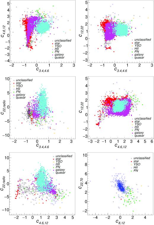
Scatter plots of selected infrared-infrared or infrared-radio colours for different infrared bands (3.4, 4.6, 12, 22, 70|$\ \mu \mathrm{m}$|). Unclassified objects are shown with grey smaller dots while pre-classified sources with coloured markers (H ii regions: blue crosses, PNe: green diamonds; stars: red stars; YSOs: orange asterisks; galaxies: purple dots, QSO: cyan triangles).
We superimposed data for different classes of objects taken from previous radio surveys cross-matched to the aforementioned infrared surveys. Radio star data (shown as red stars) at 843 MHz and 1.4 GHz are taken from Kimball & Ivezić (2008)22 and from Wendker (1995). Data for galaxy and QSO with point-like morphology at 1.4 GHz (shown respectively with purple dots and cyan triangles) are taken from Kimball & Ivezić (2008). Additionally, we included infrared data for stars, galaxies and quasars from Clarke et al. (2020), taking only sources reported with classification probability equal to 1 and requiring infrared fluxes above the AllWISE 5σ limits for all bands (Cutri et al. 2013). H ii regions (blue crosses) and PNe (green diamonds) at 843 MHz and 1.4 GHz data are taken from the Anderson et al. (2014) and HASH (Parker et al. 2016) data bases, respectively. Radio data at 5 GHz for YSO (orange asterisks) are taken from Urquhart et al. (2009). Pulsar data from the ATNF data base (Manchester et al. 2005) were also considered but since no match was found with IR data they were not reported in Fig. 12.
From Fig. 12 we observe that most colour correlations provide valuable information to separate Galactic and extragalactic sources. Longer wavelength bands are found more sensitive to object identity information for classification purposes. For example known Galactic objects tend to have larger S12, 22/S3.4, 4.6, radio flux ratios on average compared to galaxies. From the data shown in the bottom right-hand panel, one may be tempted to conclude that the sole presence of an associated 70|$\ \mu \mathrm{m}$| emission is a clear indication of the source’s Galactic origin. This is rather due to a lack of reference data for extragalactic background objects in this portion of the parameter space. Indeed, far-infrared emission (also at 70|$\ \mu \mathrm{m}$|) from several nearby galaxies was reported in different works (e.g. see Dale et al. 2012) and expected from our calculations.23
Reference data have some limitations to be considered for further analysis. First, the currently available radio data are obtained at slightly different frequencies (843 MHz, 1.4 GHz, 5 GHz) with respect to the ASKAP scorpio data (912 MHz). The introduced spread in the IR/radio colours is expected to be negligible for Galactic sources with thermal emission or flat spectra. A correction for sources with steeper spectra (expected of the order of 0.5 and 1.8 at 1.4 and 5 GHz, respectively, with α = −1) is however not possible as the spectral index information is only available for very few sources. A second limitation is that the source parameter data have many missing values for multiple reasons that cannot easily be distinguished from one another without an in-depth revision of the external catalogue data. This prevented us from encoding and imputing missing information in an effective way. For example, some catalogues do not always provide match information for all IR bands, e.g. WISE W1 and W2 information is missing in the H ii region and PN catalogues, but we may expect for a subset of these sources an emission at these wavelengths.24 Flux information may also be missing for some sources either because the reference survey covers a limited portion of the sky (e.g. radio galaxy data obtained in extragalactic surveys do not have 8 and 70|$\ \mu \mathrm{m}$| information) or because the source is not emitting or below the detection threshold. We eventually removed sources with missing data (e.g. using listwise deletion), reducing the sample size usable for analysis.
5.3.2 Classification analysis
We attempted to perform a simple source classification analysis to identify Galactic source candidates using four colour parameters (c3.4, 4.6, c4.6, 12, c12, 22, c22, radio) for which we have the largest availability of data for all bands. The resulting training sample (∼1650 sources) is unbalanced by a factor 10 towards extragalactic objects. A decision tree classifier was then trained on this data set and tested on the unclassified sample (284 sources). The optimal tree maximum depth size (3) was determined by comparing classification performances on multiple random validation samples. On the full training sample we obtained these classification metrics (recall/precision/F1-score): 0.99/0.97/0.98 for extragalactic sources and 0.69/0.89/0.78 for Galactic sources. As expected from Fig. 12, stars are the most misclassified type of object (∼70 per cent of the wrong identifications). From the decision rules it can be seen that one of the colour parameter (c12, 22) is not effectively used for the classification. Decision rules can be expressed in pseudocode as follows:

The trained tree classifies 99 sources as Galactic objects, 75 of them with classification probability larger than 90 per cent. In Fig. 13 we report the measured spectral indices for a subset (30) of them (filled red histogram) in comparison with sources classified as extragalactic (shaded blue histogram).
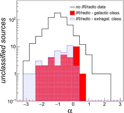
Measured spectral index for unclassified sources. The solid black line histogram includes unclassified sources for which no combined infrared-radio parameter data are available. The filled red and shaded blue histograms include unclassified sources that were classified as Galactic and extragalactic sources, respectively, in the combined infrared-radio analysis.
To make further advances we will need to individually assess the reliability of each radio-IR association (currently quoted in Section 3.2.3 as ∼60 per cent with a match radius of 8 arcsec) and possibly increase the sample of pre-classified objects to constrain the parameter space with a higher degree of confidence. Data validation efforts have already started and will be reported in a future paper.
6 SUMMARY
We have analysed ASKAP Early Science observations of the scorpio field (∼40 deg2, |$\sigma _{\rm rms}\gt 200\, \mu$|Jy beam−1, 24 × 21 arcsec angular resolution) at 912 MHz and produced a first catalogue of compact radio sources and their components using the caesar source finder. We summarize below the main results:
The catalogue contains 4144 source components with flux densities ranging from 3.9 Jy down to 0.3 mJy. About ∼87 per cent were detected at a significance higher than 5σ. From simulations, we estimated a catalogue completeness of at least 90 per cent above 5 mJy. The differential source counts are compatible with literature data at 1.4 GHz obtained outside the Galactic plane, after taking into account the different observation frequency and analysis systematics. This suggests a majority of extragalactic sources in the catalogue.
Through comparison with different radio surveys, including our ATCA observations at 1.4–2.6 GHz, we estimated the spectral indices for a subset of the catalogued sources (780) finding a median value of 〈α〉 = −0.92 (IQR = 0.68) in agreement with previous works within the discussed uncertainties. The higher resolution ATCA data also allowed us to derive a lower limit (∼8 per cent) on the fraction of the extended sources present in the catalogue.
We cross-matched the source catalogue with different astronomical data bases (SIMBAD, HASH, WISE H ii regions, Wolf–Rayet catalogue) to search for possible associations to known Galactic objects. Including candidate objects, we have found 20 stars (including 7 YSO), 21 pulsars, 38 PNe, 67 H ii regions, providing new spectral index measurements for a subsample of these, detected in both ASKAP and ATCA observations.
The vast majority (|$\gt 96\, \rm {percent}$|) of the catalogued sources are unclassified, likely dominated by extragalactic background sources. About 300 sources have been identified as radio galaxy candidates from morphological considerations. The remaining sources were analysed in correlation with existing mid-infrared data, in particular with the AllWISE survey. The majority of the unclassified sources do not have IR counterparts at 12 and 22|$\ \mu \mathrm{m}$| above IR flux sensitivity levels (∼6 mJy) within the ASKAP beam radius. About one hundred sources found with IR counterparts were preliminarily classified as Galactic objects on the basis of their radio-infrared colours. A summary of the obtained results is reported in Table E1 (available in the online version of this paper).
The source catalogue will be updated before the beginning of the ASKAP Galactic plane survey once that the scheduled Early Science data of the ASKAP scorpio field with 36 antennas at three different frequencies (920, 1296, 1630 MHz) are available and fully reduced. The multifrequency data and the expected boost in sensitivity and spatial resolution will enable us to measure the spectral index for all scorpio sources, including those located outside the ATCA survey and near the current ASKAP detection threshold, enabling further advances in our classification studies.
SUPPORTING INFORMATION
Scorpio_ASKAP15_CompactSources_finalVersion_supplMaterial.pdf
Please note: Oxford University Press is not responsible for the content or functionality of any supporting materials supplied by the authors. Any queries (other than missing material) should be directed to the corresponding author for the article.
ACKNOWLEDGEMENTS
The Australian SKA Pathfinder is part of the Australia Telescope National Facility which is managed by CSIRO. Operation of ASKAP is funded by the Australian Government with support from the National Collaborative Research Infrastructure Strategy. Establishment of the Murchison Radio-astronomy Observatory was funded by the Australian Government and the Government of Western Australia. This work was supported by resources provided by the Pawsey Supercomputing Centre with funding from the Australian Government and the Government of Western Australia. We acknowledge the Wajarri Yamatji people as the traditional owners of the Observatory site.
We thank the authors of the following software tools and libraries that have been extensively used for data reduction, analysis and visualization: askapsoft (Whiting et al. 2019), caesar (Riggi et al. 2016, 2019), astropy (Astropy Collaboration 2013, 2018), root (Brun & Rademakers 1997), topcat (Taylor 2005, 2011), ds9 (Joye & Mandel 2003), aplpy (Robitaille & Bressert 2012).
This publication makes use of data products from the Wide-field Infrared Survey Explorer, which is a joint project of the University of California, Los Angeles, and the Jet Propulsion Laboratory/California Institute of Technology, funded by the National Aeronautics and Space Administration. Additionally, this research has made use of the SIMBAD data base, operated at CDS, Strasbourg, France (Wenger et al. 2000) and the VizieR catalogue access tool, CDS, Strasbourg, France (DOI: 10.26093/cds/vizier). The original description of the VizieR service was published in Ochsenbein, Bauer & Marcout (2000).
Some of the authors benefited from grant No. 863448 (NEANIAS) of the Horizon 2020 European Commission programme. HA benefited from grant CIIC 90/2020 of Universidad de Guanajuato, Mexico. MJM acknowledges the support of the National Science Centre, Poland through the SONATA BIS grant 2018/30/E/ST9/00208.
DATA AVAILABILITY
Source tables are provided as online supplementary material.
The following catalogue data products are available in the Zenodo repository25 at http://doi.org/10.5281/zenodo.4386692:
Source catalogue in tabular format: Two ascii/FITS table files with a series of summary parameters for each catalogued source islands and fitted components, respectively. Table format (number of data columns and column description) is detailed in the caesar documentation at https://caesar-doc.readthedocs.io. Additionally, we provide an added-value source component catalogue table (ascii and FITS formats) with extra-information (corrected fluxes, radio/infrared cross-match info, spectral indices, etc.). Its format is described in Table B1 (available in the online version of this paper)
Source catalogue inrootformat: A root26 file storing the list of catalogued sources and relative components as a caesarSource C+ + object. For each source the summary parameters plus detailed information at pixel level are available. The detailed format is described in the caesar API documentation at https://caesar-doc.readthedocs.io.
Source list in region format: Two ds927 region files with the list of catalogued source islands and fitted components, respectively reported as labelled polygons or ellipses.
Background maps infitsformat: Two fits files with background and noise maps obtained in the source finding process.
Footnotes
By ‘island’ (or ‘blob’) we denote a group of connected pixels with brightness above a merge threshold and around a seed pixel with brightness above a detection threshold. Island counts include also islands nested in other islands.
10.5281/zenodo.3768398
See the WISE Explanatory Supplement at http://wise2.ipac. caltech.edu/docs/release/allsky/expsup/
Simulation tasks (compact source subtraction, point-source generation) can be performed using application scripts provided along with caesar.
The median offset was found to be 2.7 arcsec but we corrected for the systematic offset of −1 arcsec reported in Murphy et al. (2007) with respect to NVSS data.
For comparison, the angular resolution of XXL and THOR survey are 4.8 and 25 arcsec, respectively.
No bias term is included in equation (8), as we already corrected our data for measurement bias.
The minimum detection threshold value corresponds here to the 5σ threshold with respect to the minimum noise (σrms = 300 μJy beam−1) in the map, not to the ‘effective’ detection threshold, averaged over the mosaic, which amounts to ∼5 mJy.
This number refers to the number of PNe (32 True PN, 6 Likely PN, 7 Possible PN, 15 New Candidates) listed in the online HASH data ase version 4.6 (http://202.189.117.101:8999/gpne/dbMainPage.php) at the time of writing of the paper and found inside the source finding region. If we also consider the mosaic edges the PN count increases to 67 (36 True PN, 7 Likely PN, 8 Possible PN, 16 New Candidates).
We considered an average value with respect to measured PN electron temperatures found in the range 5000–15 00 K (e.g. see Zhang et al. 2014 for results on a sample of 48 Galactic PNe).
The number of H ii regions falling in the full ASKAP mosaic, including borders, is 382, as reported in paper 1 (Umana et al., in preparation).
The number of H ii regions detected in ASKAP is 261, as reported in paper 1 (Umana et al., in preparation), if we also consider the mosaic borders and the extended sources that were excluded from this catalogue.
The NASA/IPAC Extragalactic Data base (NED) (http://ned.ipac.caltech.edu) is operated by the Jet Propulsion Laboratory, California Institute of Technology, under contract with the National Aeronautics and Space Administration.
Catalogue data available at http://www.aoc.nrao.edu/∼akimball/radiocat_2.0.shtml
Following Silva et al. (1998), Michałowski et al. (2008, 2010), Iglesias-Páramo et al. (2007) we computed the expected 70|$\ \mu \mathrm{m}$| emission as a function of redshift for different SED models and compared it with the Hi-GAL detection threshold of ∼0.5 mJy (Molinari et al. 2016). For radio fluxes close to the catalogue detection threshold (∼5 mJy) only galaxies (z <0.6) with specific SED models can be detected. Above the ASKAP detection threshold we expect galaxies to be detectable at all redshifts and, thus, to populate the corresponding parameter space in Fig. 12
We visually inspected some of the catalogued H ii regions in all WISE bands. The infrared emission in bands W1 and W2 was effectively found absent or not correlated with the W3 and W4 emission but we cannot exclude such a correlation for the rest of catalogued objects that were not inspected. In fact in Assef et al. (2018) the authors conservatively removed the areas of the sky around WISE H ii regions to eliminate the Galactic source background when searching for potential AGN in W1 and W2 bands. An emission at these shorter wavelengths, albeit smaller compared to W3 and W4 bands, can be therefore present and was indeed observed in some of the H ii regions catalogued by CORNISH (Purcell et al. 2013) (for example in G019.6062-00.9018)
