


ABSTRACT
We present modelling of the long-term optical light and radial velocity curves of the binary stellar system CXOGBS J175553.2−281633, first detected in X-rays in the Chandra Galactic Bulge Survey. We analysed 7 yr of optical I-band photometry from Optical Gravitational Lensing Experiment and found long-term variations from year to year. These long-term variations can most likely be explained with by either variations in the luminosity of the accretion disc or a spotted secondary star. The phased light curve has a sinusoidal shape, which we interpret as being due to ellipsoidal modulations. We improve the orbital period to be P = 10.34488 ± 0.00006 h with a time of inferior conjunction of the secondary star T0 = HJD 2455260.8204 ± 0.0008. Moreover, we collected 37 spectra over 6 non-consecutive nights. The spectra show evidence for an evolved K7 secondary donor star, from which we obtain a semi-amplitude for the radial velocity curve of K2 = 161 ± 6 km s−1. Using the light-curve synthesis code xrbinary, we derive the most likely orbital inclination for the binary of i = 63.0 ± 0.7 deg, a primary mass of M1 = 0.83 ± 0.06 M⊙, consistent with a white dwarf accretor, and a secondary donor mass of M2 = 0.65 ± 0.07 M⊙, consistent with the spectral classification. Therefore, we identify the source as a long orbital period cataclysmic variable star.
1 INTRODUCTION
Cataclysmic variables (CVs) are binary star systems composed of a white dwarf primary accreting matter from a main sequence or evolved secondary star (Patterson 1984; Warner 1995; Kalomeni et al. 2016). Low-mass X-ray binaries (LMXBs) are analogous systems where the primary is either a black hole or a neutron star, instead of a white dwarf (Remillard & McClintock 2006). There are only about 20 dynamically confirmed black hole X-ray binaries known in the Milky Way (e.g. Casares & Jonker 2014). Finding and modelling CVs and LMXBs allows us to better understand the formation of compact objects and test binary evolution models (Jonker & Nelemans 2004; Repetto & Nelemans 2015).
The Chandra Galactic Bulge Survey (GBS) is a survey tasked with finding more quiescent LMXBs. Towards this goal the GBS covered a total of 12 deg2 near the Bulge of our galaxy and found 1640 X-ray sources (Jonker et al. 2011, 2014). Subsequent studies have identified counterparts to these sources in multiple wavelengths; from radio (Maccarone et al. 2012) and near-infrared (Greiss et al. 2014) to optical (Hynes et al. 2012; Udalski et al. 2012; Britt et al. 2014; Wevers et al. 2016b, 2017). Some of these counterparts have been deemed likely accreting binaries, motivating further photometric and spectroscopic follow up (Ratti et al. 2013; Wevers et al. 2016a; Johnson et al. 2017).
In this work, we focus on one of these objects, CXOGBS J175553.2−281633 (hereafter CX137). The optical counterpart to CX137 was first identified by Udalski et al. (2012) and classified as an eclipsing binary with a spotted donor star and an orbital period of 10.345 h. Subsequent spectroscopic and photometric follow up by Torres et al. (2014) revealed broad Hα emission and an orbital period consistent with that of Udalski et al. (2012). Based on the properties of the Hα emission line and an X-ray luminosity of Lx > 5.8 × 1030 erg s−1, Torres et al. (2014) classified the source as a potential low-accretion rate CV or quiescent LMXB with a G/K-type secondary, supporting the ellipsoidal light-curve interpretation.
In this work, we build on the analysis from Torres et al. (2014) by including two extra years of I-band photometry, where the sinusoidal shape of the light curve can be explained by ellipsoidal modulations. Additionally, we see long-term variations in the shape of the light curve, these are consistent with either changes in the luminosity of an accretion disc or a spotted secondary star. In this work, we aim to settle the true nature of the object by performing a dynamical study and find that CX137 is a CV with a K7 secondary star and an orbital period of P = 10.34488 ± 0.00006 h, in agreement with previous studies. The source shows no outbursts in our seven years of optical photometry.
This paper is organized as follows: in Section 2, we describe the OGLE (Optical Gravitational Lensing Experiment) photometry and the optical spectroscopy obtained for this study. In Section 3, we provide an analysis of the data; where we determine the orbital period, generate a radial velocity curve for the secondary star, and describe the spectral features. In Section 4, we present our light-curve models, fitting routines, and resulting output parameters. We finally outline our discussion in Section 5 and conclusion in Section 6. All quoted errors in this paper represent 1σ uncertainty, unless otherwise stated.
2 OBSERVATIONS
2.1 Gaia
Gaia provides precise coordinates for the optical component of CX137 at RA = 17h55m53s.26, Dec. = −28°16′33″.84 (ICRS), in addition to proper motion components of μRA = 1.139 ± 0.108 mas yr−1, and μDec. = −6.977 ± 0.087 mas yr−1. The parallax of the source was measured by Gaia DR2 to be π = 1.116 ± 0.069 mas, which corresponds to a distance of |$d = 879^{+59}_{-52}$| pc (Bailer-Jones et al. 2018; Gaia Collaboration et al. 2018).
2.2 OGLE photometry
The optical counterpart of CX137 was observed during the fourth phase of the OGLE project with the 1.3-m Warsaw telescope at Las Campanas Observatory (Udalski, Szymański & Szymański 2015). OGLE provided us with 7 yr of I-band photometry, from 2010 to 2016. The typical cadence of these observations ranges from 20 min to nominally once a night with exposure times of 100 s. There is a three month period in each year when the source is not visible. The photometry was obtained using the difference image analysis method outlined in Wozniak (2000). The individual photometry has typical errors of <0.01 mag, see Table 1 for a log of observations.
OGLE I-band photometry. All exposure times were 100 s.
| UT date range | Exposures |
|---|---|
| 2010 Mar 5–Nov 4 | 1685 |
| 2011 Feb 3–Nov 9 | 2042 |
| 2012 Feb 3–Nov 11 | 936 |
| 2013 Feb 3–Oct 30 | 868 |
| 2014 Feb 1–Oct 26 | 848 |
| 2015 Feb 7–Nov 7 | 804 |
| 2016 Feb 6–Oct 30 | 1641 |
| UT date range | Exposures |
|---|---|
| 2010 Mar 5–Nov 4 | 1685 |
| 2011 Feb 3–Nov 9 | 2042 |
| 2012 Feb 3–Nov 11 | 936 |
| 2013 Feb 3–Oct 30 | 868 |
| 2014 Feb 1–Oct 26 | 848 |
| 2015 Feb 7–Nov 7 | 804 |
| 2016 Feb 6–Oct 30 | 1641 |
2.3 Optical spectroscopy
We observed CX137 with the Intermediate dispersion Spectrograph and Imaging System (ISIS; Jorden 1990) on the 4.2-m William Herschel Telescope (WHT) at the Roque de los Muchachos Observatory on La Palma, Spain, during five different observing runs between 201 7June and August. The ISIS spectrograph has a dichroic that splits the spectra into a red and blue arm, allowing for a wide spectral range to be observed simultaneously. For the blue arm, we used gratings R158, R300, and R600; and for the red arm, we used gratings of R158 and R600. We also obtained one high-resolution spectrum with the Inamori-Magellan Areal Camera and Spectrograph (IMACS; Dressler et al. 2011) on the Magellan Baade 6.5 m Telescope at Las Campanas observatory with the R1200 grating. We provide a log of spectroscopic observations and specifications of each grating in Table 2. The spectral resolutions provided in the table were approximated by measuring the width of spectroscopic lines in an arc lamp spectrum taken with each grating.
Optical spectroscopy of CX137.
| UT date | Exposure | Telescope + | Grating | Dispersion | Resolution | Slit width | Wavelength range | |
|---|---|---|---|---|---|---|---|---|
| (s) | Instrument | (lines mm−1) | (Å pixel−1) | (Å) | (km s−1) | (arcsec) | (Å) | |
| 2017 Jun 24 | 6 × 600 | WHT + ISIS-red | R158 | 1.81 | 7.70 | 307 | 1.0 | 5500–8100 |
| 2017 Jun 24 | 6 × 600 | WHT + ISIS-blue | R158 | 1.62 | 7.81 | 520 | 1.0 | 3500–5400 |
| 2017 Jul 11 | 6 × 600 | WHT + ISIS-red | R158 | 1.81 | 7.70 | 307 | 1.0 | 5500–8100 |
| 2017 Jul 11 | 6 × 600 | WHT + ISIS-blue | R300 | 0.86 | 4.10 | 273 | 1.0 | 3500–5400 |
| 2017 Jul 21 | 15 × 900 | WHT + ISIS-red | R600 | 0.49 | 1.81 | 72 | 1.0 | 5500–8800 |
| 2017 Jul 21 | 15 × 900 | WHT + ISIS-blue | R600 | 0.45 | 2.02 | 134 | 1.0 | 3500–5400 |
| 2017 Aug 27 | 3 × 900 | WHT + ISIS-red | R600 | 0.49 | 1.81 | 72 | 1.0 | 5500–7150 |
| 2017 Aug 27 | 3 × 900 | WHT + ISIS-blue | R600 | 0.45 | 2.02 | 134 | 1.0 | 3910–5400 |
| 2017 Aug 29 | 4 × 900 | WHT + ISIS-red | R600 | 0.49 | 1.81 | 72 | 1.0 | 5500–7150 |
| 2017 Aug 29 | 4 × 900 | WHT + ISIS-blue | R600 | 0.45 | 2.02 | 134 | 1.0 | 3910–5400 |
| 2017 Oct 8 | 3 × 900 | Magellan + IMACS | R1200 | 0.376 | 1.54 | 54 | 0.9 | 8500–8900 |
Notes: the spectral resolution is measured at 4500 Å for the ISIS-blue arm, 7500 Å for the ISIS-red arm, and 8600 Å for IMACS. The wavelength range represents only the high-quality portion of the spectra used for our analysis.
We reduced the spectra using standard iraf1 routines. The data were bias-subtracted and flat-fielded, sky emission subtracted, the spectra were optimally extracted and wavelength calibrated using an arc lamp taken after each spectrum. We determine the zero-point of the wavelength calibration of our spectra by measuring the positions of bright sky lines in each spectrum, and apply the corresponding shift to each individual spectrum such that the wavelength of the sky lines match between all the spectra. For the ISIS spectroscopy, we analysed the data taken in both the red and blue arms using the same procedure, but treat them as individual spectra.
2.4 Spectral templates
Throughout this work, we make use of spectral templates from the X-shooter library (Chen et al. 2011). We selected spectra from 71 M, 33 K, and 23 G stars of varying luminosity classes and evolutionary stages. All templates were taken with a 0.7 arcsec slit with the VIS arm of X-shooter and a nominal resolution of R ∼10 000, equivalent to ∼30 km s−1 at a wavelength of 8600 Å.
All the spectra of CX137 and templates were subsequently processed using molly.2 First, we apply a heliocentric velocity correction to all spectra using the hfix task. We then use vbin to bin all the data to a uniform velocity scale so the dispersion of the templates matches that of the CX137 spectra. We then normalize each spectrum by dividing it by a fit to the star’s continuum. To estimate the continuum we fit a second-order polynomial to each spectrum, masking out regions with strong emission lines or telluric bands.
3 DATA ANALYSIS
3.1 Photometric periodicities
We use all 7 yr of OGLE I-band photometry to determine the orbital period of the binary. For this, we employ the gatspy python package (VanderPlas & Ivezić 2015), which provides an implementation of the Lomb–Scargle periodogram to find periodicities in the photometric data. The strongest peak of the periodogram is at a period of P = 5.17244 h. When the data are phase-folded at this period we see large scatter in the light curve, which is due to the fact that the maxima expected from ellipsoidal modulations at phase 0.25 and 0.75 have different strengths (see Fig. 1). Fig. 1 shows the light curve phase-folded at a period of twice that of the corresponding strongest peak, P = 10.34488 ± 0.00006 h, consistent with the period found in Udalski et al. (2012) and Torres et al. (2014). Motivated by the fact that spin periods in the range of 0.1–10 per cent of the orbital period have previously been observed in magnetic CVs (Norton, Wynn & Somerscales 2004), we search for periodicities in the 100–20 000 s range with null results. We detect no measurable change in the orbital period over our 7 yr baseline. On the other hand, we detect a possible long-term trend at a period of ∼796 d. Since the full span of the light curve is only three times this period, more data are required to confirm if this is a real periodicity or just a temporary artefact. The data phase-folded at this period is shown in the bottom panel of Fig. 1.
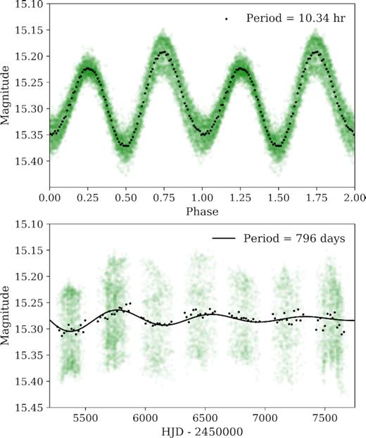
Top: optical photometry phased at the best orbital period of P = 10.34488 h. Bottom: full OGLE light curve where long-term periodic variations in luminosity are seen. The green dots are all the data, while the black dots are binned in phase bins of 0.01 for the phased light curve and bins of 20 d for the full light curve. We show a tentative period of 796 d as a damped sine curve fit to the binned data. The error bars are approximately equal to the size of the data points and are not plotted for clarity.
3.2 Spectral type of the secondary
Fig. 2 shows the blue and red normalized ISIS spectra of CX137 averaged in the rest frame of the secondary star. The spectra are mostly dominated by absorption lines from the secondary, with additional Balmer emission lines from an accretion disc. We detect the Mg triplet absorption lines from the secondary, and interstellar Na D lines. We see a weak contribution from TiO bands of the secondary in the ∼6100–6300 Å range, and no evidence for He i emission lines, which are common in CVs (e.g. Rodríguez-Gil et al. 2009; Ratti et al. 2013). This might be due to the lines being veiled by a large flux contribution from the secondary. We can set an upper limit to the absolute equivalent width of He i λ7065 to be <1.6 Å, and <1.2 Å for He ii λ4686.
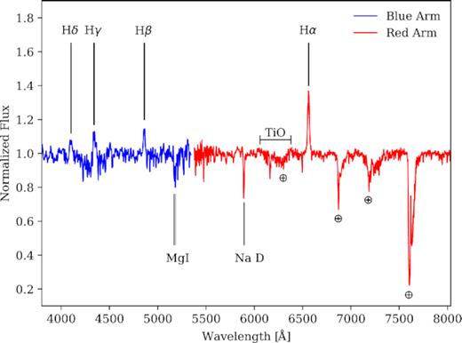
Average continuum-normalized blue and red arm ISIS spectrum for CX137 in the rest frame of the secondary. The spectra show Balmer lines in emission, associated with the accretion disc. Strong stellar features are indicated. The interstellar Na D is also marked. ⊕ denotes prominent telluric features.
To estimate the temperature of the secondary star, we first average all the CX137 ISIS data taken with the R600 grating to use as a high S/N reference. We compare this spectrum to that of the X-shooter templates described in Section 2.4. First, we corrected each template spectrum for the systemic velocity of each star and broaden it by convolving it with a Gaussian function to match the spectral resolution of the ISIS data. We subtract each template to the normalized CX137 spectrum in the 5580–6150 Å wavelength range (masking out telluric lines and emission lines not associated with the secondary), and search for the template star that produces the lowest residuals, allowing for a varying multiplicative f factor, which represents the fractional contribution of the template star from the total flux. We find that the spectrum of CX137 best matches that of HD79349, a K7IV star with a temperature of 3850 ± 30K, and a systemic velocity of 47.12 ± 0.15 km s−1 (Gaia Collaboration et al. 2018; Arentsen et al. 2019). We find a best fit for the average optimum factor of f = 0.52 ± 0.06.
3.3 Radial velocities
To measure the radial velocity of the secondary in each spectrum we use the xcor task in molly to cross-correlate the CX137 spectra with the spectrum of the K7IV star HD79349, the template star that best matches the spectra of CX137 (described in Section 2.3). The actual choice of template star does not have a noticeable effect in the measured radial velocities. We correct the template star’s spectrum for its systemic velocity and broaden it by convolving it with a Gaussian function to match the spectral resolution of the CX137 spectra. We consider the wavelength range listed in Table 2 for each CX137 spectrum, masking out telluric features and emission lines not associated with the secondary before cross-correlating them. We calculate the radial velocities from both the red and blue arms data of the ISIS spectrograph independently. The resulting radial velocity curve is shown in Fig. 3, with the individual measurements provided in Table A1. We note that the radial velocities measured near phase 0.25 have a large scatter due to noisy spectra taken in poor weather conditions.
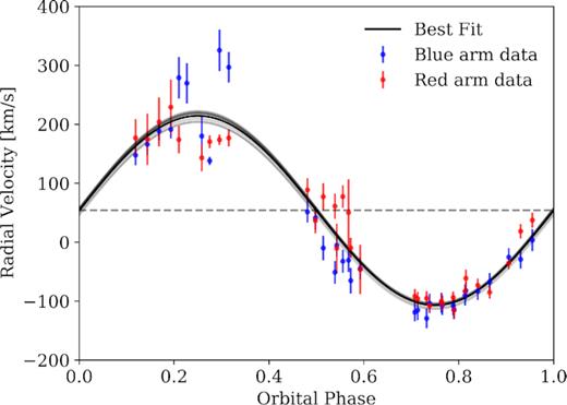
Heliocentric radial velocity curve measured from both the blue and red arms of ISIS spectra. The best-fitting sine curve is shown in black. The dashed horizontal line marks the 0 point of the sinusoid. The best-fitting values to the systemic radial velocity and semi-amplitude of the radial velocity are γ = 54 ± 4 km s−1 and K2 = 161 ± 6 km s−1, respectively.
3.4 Rotational broadening of the secondary star
To estimate the rotational broadening of the secondary we compare the set of spectral templates described in Section 2.4 to the high-resolution IMACS spectrum of CX137 taken near photometric orbital phase 0. We normalize the IMACS and X-shooter spectra by dividing them by a second-degree polynomial fit to their respective continuum (masking out absorption features) in the 8500–8900 Å range. We scale down the resolution of the X-shooter templates to match that of the IMACS spectrum by convolving them with a Gaussian function. We then broaden the templates by a range of velocities from 20 to 200 km s−1 in steps of 1 km s−1 using the rbroad task in molly. This task takes the input spectrum and broadens it through convolution with the rotational profile of Gray (1992), where we adopt a limb-darkening coefficient of 0.75. Finally, we subtract the broadened templates from the CX137 spectrum, following the same procedure as described in Section 2.3. Through χ2 minimization we find a best fit of vsin (i) = 101 ± 3 km s−1 to the rotational velocity of the secondary star in CX137. We find the best match to be comparably good for a K4III, K3.5III, K2III, and K7IV template star. G and M stars produce statistically worst fits. The individual vsin (i) measurements are shown in Table 3.
Rotational broadening of CX137 for different templates.
| Star | Spectral type | v sin (i) | f |
|---|---|---|---|
| (km s−1) | |||
| HD37763 | K2III | 99 ± 3 | 0.48 ± 0.06 |
| HD79349 | K7IV | 100 ± 3 | 0.41 ± 0.03 |
| BS4432 | K3.5III | 100 ± 3 | 0.52 ± 0.04 |
| HD74088 | K4III | 104 ± 3 | 0.50 ± 0.04 |
| Star | Spectral type | v sin (i) | f |
|---|---|---|---|
| (km s−1) | |||
| HD37763 | K2III | 99 ± 3 | 0.48 ± 0.06 |
| HD79349 | K7IV | 100 ± 3 | 0.41 ± 0.03 |
| BS4432 | K3.5III | 100 ± 3 | 0.52 ± 0.04 |
| HD74088 | K4III | 104 ± 3 | 0.50 ± 0.04 |
Note: f is the corresponding optimum factor measured in the 8500–8900 Å range.
4 LIGHT-CURVE MODELLING
We proceed to model the optical light curve of CX137 using xrbinary,3 a light-curve synthesis code developed by Robinson. This code assumes a binary system composed of a compact primary and a co-rotating secondary star that fills its Roche Lobe and is transferring mass via an accretion disc. The code models the tidal distortion of the secondary (responsible for the ellipsoidal modulations), and accounts for irradiation of the surface of the secondary from the bright accretion disc. The accretion disc is assumed to be optically thick and to emit as a multitemperature blackbody. The disc’s temperature profile as a function of radius is given by an equation of the form T4∝R−3(1 − (Rin/R)0.5), where Rin is the inner disc radius. In order to account for the observed symmetries in the light curve, we model the photometry of CX137 with three different models: (i) a model with a Roche Lobe filling secondary and an accretion disc that is allowed to vary in luminosity and eccentricity, (ii) a similar model, but with a circular accretion disc where the temperature of the edge of the disc can have a hot and a cool side, and (iii) a model with a circular accretion disc and an edge of uniform temperature, but with two spots on the surface of the secondary. For all models we fit the light curve using the emcee Markov Chain Monte Carlo (MCMC) sampler (Foreman-Mackey et al. 2013).
The relevant parameters of the model are: the inclination of the system i; an orbital phase shift of the photometric T0 with respect to the spectroscopic T0, ϕ; the temperature of the secondary star T2; the temperature of the edge of the accretion disc TE; the mass ratio q = M2/M1; the argument of periastron of the disc ωD; the outer disc radius RD; the disc luminosity LD; the height of the accretion disc HD; the eccentricity of the accretion disc eD; the temperature ratio between the hot and cool sides of the disc edge Th; the width of the hot side of the disc edge Wh; the location of the centre of the hot edge of the disc θh; the polar coordinates of the first and second spots on the surface of the secondary ϕS1, θS1, ϕS2, and θS2, respectively; the temperature ratio between the spots’ temperature and the secondary temperature TS1, and TS2 respectively, and the size of the spots RS1, and RS2. Only the relevant parameters are included in each of the three versions of the models described in the following section.
In all models we fix the semi-amplitude of the radial velocity of the secondary to K2 = 161 km s−1 (derived in Section 3.3). We use wide uniform priors for ϕ, T2, TE, ωD, RD, eD, Wh, and all the parameters pertaining to the spots. For LD we use a prior that is flat in log space to allow for even sampling of the parameter space across orders of magnitude. For i we use a prior that is flat in cos (i). We implement a Gaussian prior on the mass ratio centred at q = 0.79 ± 0.06 (derived in Section 3.4). We restrict the accretion disc to be larger than the circularization radius Rc = (1 + q)(0.5 − 0.227log (q))4 (Frank, King & Raine 2002). Finally, apply a flat prior on the temperature of the secondary of T2 = [3500, 4100], based on the temperature of the template star that best matches the spectra of CX137 (derived in Section 2.3). The xrbinary code interpolates the temperature from a table of Kurucz models, therefore the measurement of the temperature of the secondary is not very precise (±125 K), we report only the statistical model uncertainties in Table 5.
In order to account for the year-to-year variations in the light curve we separate the photometry into eight epochs, nominally one for every year of data. Dividing the photometry into eight epochs allows us to roughly track the evolution of the system, assuming the parameters of the system are approximately constant in the ∼8 months of data each epoch spans (see Fig. 1). We see the shape of the light curve does remain fairly constant within each epoch, except for the 2016 epoch, which we therefore split into two epochs of equal time span named 2016a and 2016b, each of which do have a stable light-curve shape. Subdividing the epochs further proved to be too computationally expensive.
4.1 Model 1: variable disc
For the first model, we allow the accretion disc to vary in luminosity and eccentricity, but do not include any spots on the disc or the secondary. For all epochs, we keep i, ϕ, T2, K2, TE, and q constant but allow the parameters that define the accretion disc ωD, RD, LD, and eD, HD to vary from epoch to epoch. The temperature of the edge of the disc TE could conceivably change from epoch to epoch, but since this parameter has little to no effect on the output light curve we constrain it to always be the same for computational purposes.
First, we fit each epoch of photometry independently, we then use the posterior distribution of those MCMC chains as starting positions when fitting all eight epochs simultaneously. We run the MCMC sampler for 1600 steps with 400 walkers and discard the first 50 per cent as burn-in. We test for convergence by using the Gelman–Rubin statistic and see that the potential scale reduction factor is |$\hat{R} \lt 1.3$| (Gelman & Rubin 1992). The most likely values are shown in Table 4. We see that the posterior distribution of all the relevant parameters is mostly Gaussian.
Best-fitting model parameters for each epoch.
| Parameter | Prior | 2010 | 2011 | 2012 | 2013 | 2014 | 2015 | 2016a | 2016b |
|---|---|---|---|---|---|---|---|---|---|
| Model 1: variable disc | |||||||||
| ϕ† | [ − 0.1–0.1] | 0.001 ± 0.002 | ⋅⋅⋅ | ⋅⋅⋅ | ⋅⋅⋅ | ⋅⋅⋅ | ⋅⋅⋅ | ⋅⋅⋅ | ⋅⋅⋅ |
| TE[K]† | [500–5000] | |$2301^{+2000}_{-500}$| | ⋅⋅⋅ | ⋅⋅⋅ | ⋅⋅⋅ | ⋅⋅⋅ | ⋅⋅⋅ | ⋅⋅⋅ | ⋅⋅⋅ |
| log (LD/[erg s−1]) | [30–35] | 33.44 ± 0.05 | 33.68 ± 0.11 | 33.67 ± 0.14 | 34.06 ± 0.3 | 33.52 ± 0.08 | 33.46 ± 0.04 | 33.46 ± 0.46 | 33.57 ± 0.14 |
| eD | [0.0–0.9] | 0.15 ± 0.04 | 0.49 ± 0.03 | 0.52 ± 0.03 | 0.58 ± 0.05 | 0.11 ± 0.07 | 0.21 ± 0.03 | 0.46 ± 0.11 | 0.08 ± 0.05 |
| |$\omega _D (\rm deg)$| | [0–360] | 12.21 ± 3.58 | 108.13 ± 2.9 | 96.21 ± 4.49 | 83.15 ± 8.74 | 17.85 ± 19.97 | 100.63 ± 7.09 | 73.14 ± 4.67 | 78.12 ± 21.11 |
| RD[Rc] | [1.0–3.0] | 1.30 ± 0.03 | 1.03 ± 0.03 | 1.01 ± 0.02 | 1.02 ± 0.03 | 1.48 ± 0.10 | 1.99 ± 0.09 | 1.33 ± 0.23 | 2.10 ± 0.21 |
| HD[a] | [0.005–0.1] | 0.009 ± 0.002 | 0.029 ± 0.001 | 0.028 ± 0.001 | 0.027 ± 0.001 | 0.019 ± 0.003 | 0.046 ± 0.003 | 0.041 ± 0.005 | 0.041 ± 0.004 |
| f* | 0.52 ± 0.02 | 0.48 ± 0.03 | 0.52 ± 0.03 | 0.49 ± 0.03 | 0.49 ± 0.02 | 0.52 ± 0.02 | 0.55 ± 0.03 | 0.48 ± 0.02 | |
| Model 2: asymmetrical disc brightness | |||||||||
| log (LD/[erg s−1]) | [30–35] | 32.94 ± 0.09 | 33.06 ± 0.10 | 33.19 ± 0.20 | 32.99 ± 0.2 | 33.16 ± 0.08 | 32.95 ± 0.08 | 32.90 ± 0.25 | 33.11 ± 0.16 |
| RD[Rc] | [1.0–3.0] | 1.45 ± 0.16 | 1.57 ± 0.08 | 1.52 ± 0.17 | 1.52 ± 0.16 | 1.43 ± 0.10 | 1.56 ± 0.14 | 1.47 ± 0.18 | 1.36 ± 0.13 |
| HD[a] | [0.005–0.1] | 0.027 ± 0.002 | 0.028 ± 0.003 | 0.030 ± 0.003 | 0.028 ± 0.004 | 0.026 ± 0.007 | 0.028 ± 0.006 | 0.029 ± 0.006 | 0.029 ± 0.007 |
| TE | [500, 5000] | 1664 ± 180 | 1669 ± 104 | 1772 ± 97 | 1762 ± 113 | 1647 ± 203 | 1706 ± 182 | 1671 ± 150 | 1474 ± 132 |
| Th | [1.0–10.0] | 1.97 ± 0.20 | 2.23 ± 0.16 | 2.27 ± 0.13 | 2.33 ± 0.17 | 2.08 ± 0.24 | 2.03 ± 0.20 | 2.13 ± 0.18 | 2.04 ± 0.10 |
| θh[deg] | [0.0–180] | 10.7 ± 1.7 | 102.3 ± 0.7 | 88.3 ± 0.7 | 61.7 ± 0.5 | 13.4 ± 1.6 | 150.0 ± 1.1 | 70.3 ± 1.5 | 100.9 ± 3.1 |
| Wh[deg] | [0.0–300] | 149.7 ± 3.4 | 177.2 ± 10.6 | 98.4 ± 2.2 | 168.3 ± 0.004 | 249.9 ± 16.8 | 188.3 ± 3.8 | 196.9 ± 5.1 | 119.0 ± 19.0 |
| f* | 0.58 ± 0.02 | 0.53 ± 0.02 | 0.49 ± 0.02 | 0.55 ± 0.02 | 0.49 ± 0.02 | 0.58 ± 0.02 | 0.60 ± 0.02 | 0.52 ± 0.02 | |
| Model 3: spotted secondary | |||||||||
| |$R_D [R_c^\dagger ]$| | [1.0 − 3.0] | 1.48 ± 0.01 | ⋅⋅⋅ | ⋅⋅⋅ | ⋅⋅⋅ | ⋅⋅⋅ | ⋅⋅⋅ | ⋅⋅⋅ | ⋅⋅⋅ |
| HD[a]† | [0.005–0.1] | 0.030 ± 0.001 | ⋅⋅⋅ | ⋅⋅⋅ | ⋅⋅⋅ | ⋅⋅⋅ | ⋅⋅⋅ | ⋅⋅⋅ | ⋅⋅⋅ |
| log (LD/[erg s−1]) | [30–35] | 33.65 ± 0.07 | 32.74 ± 0.01 | 33.57 ± 0.09 | 33.49 ± 0.08 | 33.70 ± 0.06 | 33.22 ± 0.07 | 33.43 ± 0.09 | 33.47 ± 0.07 |
| TE | [500–5000] | 2223 ± 150 | 4509 ± 21 | 2959 ± 122 | 3007 ± 113 | 2358 ± 185 | 2363 ± 137 | 2239 ± 201 | 2392 ± 165 |
| θS1 | [0–250] | 170.4 ± 2.5 | 68.2 ± 1.6 | 153.1 ± 3.1 | 162.9 ± 2.8 | 163.1 ± 5.4 | 51.7 ± 1.9 | 146.4 ± 2.2 | 143.1 ± 7.2 |
| ϕS1 | [ − 110–110] | −80.8 ± 3.1 | −55.2 ± 2.6 | −99.9 ± 2.4 | −91.1 ± 4.3 | −94.0 ± 42.9 | −45.5 ± 3.5 | −93.6 ± 1.9 | −88.3 ± 5.9 |
| RS1 | [0.0–20.0] | 12.5 ± 0.4 | 13.7 ± 1.4 | 16.0 ± 0.9 | 16.9 ± 0.7 | 12.7 ± 1.5 | 14.3 ± 0.9 | 16.3 ± 1.1 | 9.5 ± 2.8 |
| TS1 | [0.1–1.0] | 0.5 ± 0.2 | 0.4 ± 0.2 | 0.4 ± 0.1 | 0.4 ± 0.2 | 0.5 ± 0.2 | 0.5 ± 0.1 | 0.3 ± 0.2 | 0.6 ± 0.3 |
| θS2 | [0–250] | 64.2 ± 2.9 | 88.2 ± 0.3 | 80.9 ± 1.6 | 88.5 ± 1.5 | 109.9 ± 8.4 | 62.1 ± 1.2 | 94.2 ± 1.3 | 99.3 ± 2.8 |
| ϕS2 | [70–290] | 209.4 ± 5.3 | 159.9 ± 1.7 | 116.8 ± 2.4 | 157.4 ± 3.9 | 159.4 ± 18.6 | 174.5 ± 4.7 | 157.4 ± 3.8 | 160.9 ± 8.7 |
| RS2 | [0.0–20.0] | 6.9 ± 0.7 | 12.9 ± 0.2 | 16.1 ± 0.7 | 14.4 ± 0.2 | 4.1 ± 0.5 | 10.7 ± 0.5 | 10.9 ± 0.2 | 6.8 ± 0.4 |
| TS2 | [0.1–1.0] | 0.5 ± 0.2 | 0.5 ± 0.1 | 0.4 ± 0.1 | 0.5 ± 0.1 | 0.4 ± 0.2 | 0.6 ± 0.2 | 0.4 ± 0.2 | 0.6 ± 0.2 |
| f* | 0.43 ± 0.02 | 0.69 ± 0.02 | 0.46 ± 0.02 | 0.49 ± 0.02 | 0.41 ± 0.02 | 0.59 ± 0.02 | 0.51 ± 0.02 | 0.50 ± 0.02 | |
Notes: Best model parameters and 1σ error bars for the realizations shown in Fig. 4. The parameters of the disc are: the orbital phase ϕ, the luminosity LD, the eccentricity eD, the argument of periastron ωD, the disc radius RD in units of the circularization radius Rc, and edge height HD in units of semi-major axis a, and the temperature of the edge of the disc TE. We also include the fractional contribution of the donor star to the total flux of the system f, calculated in V band from the posterior distribution of the other parameters from the model. The uncertainties are purely statistical error bars obtained from the posterior distribution of the MCMC. For most parameters we adopt a flat prior, except for the disc luminosity, which is flat in log (LD). The disc radius RD is limited to be less than 0.9 times the Roche Lobe radius of the primary R1.
*These parameters were not fit for, but were calculated using all the posterior distribution samples of the fitted parameters.
†These parameters are kept constant throughout all epochs.
For this model, we interpret the changes in the light curve as being due to an accretion disc of varying shape and luminosity. We see the light curves are well modelled by a disc that gets smaller and more eccentric from 2010 to 2013, and then recedes back to its original luminosity 3 yr later and circularizes into a less eccentric disc. The best-fitting parameters for each epoch are shown in Table 4. We find a best fit for the secondary temperature of 4055 ± 25 K and a secondary mass of M2 = 0.62 ± 0.04 M⊙, both consistent with a K7 star (Cox 2000) and in agreement with the spectral classification performed in Section 2.3. The large Roche Lobe radius of the secondary R2 = 0.92 ± 0.09 R⊙ implies it must be evolved in order to fill its Roche Lobe (discussed further in Section 5).
We note that some of the best-fitting eccentricity measurements are as high as e = 0.58, which is not expected for a low accretion-rate CV with a accretion disc of radius ∼Rc, and for the high mass ratio found for CX137 of q > 0.7 (e.g, Warner 1995). For this reason, we proceed to model the light curve with a disc that is forced to be circular, but with an edge that has two zones of independent temperature.
4.2 Model 2: asymmetrical disc edge brightness
In this model, we fix the eccentricity of the disc e and argument of periastron ωD to be 0. In the previous variable disc model, we found the phase shift ϕ to be consistent with 0 with an uncertainty in phase shift of just 0.002, we therefore also fix this parameter to 0 for computational purposes. In this model, we allow the disc edge to have two different temperatures. We model this in xrbinary by using a ‘spot’ that is allowed to cover an arbitrary width of the edge of the disc, effectively creating a hot and a cool zone on the outer edge of the disc. Physically, this could be produced by the impact of the gas stream on the disc, which causes the region near the impact hotspot to be hotter than the region on the opposite side of the disc. Changes in the mass transfer rate from the secondary can affect the temperature of this ‘spot’ (e.g. SDSS J123813.73−033933.0, Zharikov et al. 2006), which could be responsible for the observed year to year variations and the ∼796 d periodicity derived in Section 3.1.
In this model, we fit for the temperature ratio between the hot and cool sides of the disc edge Th, the width of the hot side of the disc edge Wh, and the location of the centre of the hot edge of the disc θh; these last two measured in degrees. θh is defined such that θh = 0 deg is the direction pointing from the primary straight away from the secondary, and θh = 90 deg points towards the observer at phase 0.75, when the observer sees the side of the disc where we would expect an accretion hotspot to be.
We fit the model in the same way as described in Section 4.1, in this case running the MCMC with 2000 steps and 400 walkers, and also discarding the first 50 per cent as burn-in. The resulting model has an |$\hat{R} \lt 1.4$|. The most likely values are shown in Table 4. We see a correlation between Wh and Th, since a large hot zone can produce a similar light curve to a smaller zone with a higher temperature. These parameters are also correlated with the disc height HD, which together with Wh define the effective area of the hot zone. The best-fitting disc radius is ∼1.5Rc throughout all epochs, and a hot region that covers ≳ 100 deg of the edge of the disc. Models predict that for the best-fitting parameters of CX137, a typical hotspot would cover ≲ 5 deg of the edge of the disc (Livio 1993). From observations, Warner (1995) find spots that cover the range of 14–40 deg, much smaller than what we measure for CX137.
We find a best fit for the secondary temperature of 3814 ± 20 K and a secondary mass of M2 = 0.68 ± 0.03 M⊙. A cooler but more massive star is not necessarily consistent with the K7 secondary we expect from our spectral analysis in Section 2.3. Allowing the disc to be hotter effectively lowered the temperature of the secondary to the point where this model is not entirely self-consistent, and therefore disfavored. This model can help towards a better understanding of the systematic uncertainties in measuring M1, M2, and i. Finally, we explore a third model in which the accretion disc is circular and the disc edge has one uniform temperature, but we include two spots on the surface of the secondary.
4.3 Model 3: spotted secondary
Finally, we fit the light curves with a model in which the accretion disc is forced to be circular, and have an edge with a single temperature, fixing Wh = 0, θh = 0, and Th = 1. We place two spots on the surface of the secondary with polar coordinates ϕS1, θS1, ϕS2, and θS2, respectively; and fix −110 deg < ϕS1 < 110 deg, and 70 deg < ϕS2 < 290 deg. This prior effectively constrains spot 1 to be on the side of the secondary facing the observer during orbital phase 0.75, and spot 2 on the opposite side of the secondary, allowing for a small overlap region of 20 deg. The spots have respective angular sizes RS1, and RS2, and a temperature ratio with respect to the secondary TS1, and TS2, which are constrained to be <1. We fit for the size and height of the disc as in the previous models, but for computational purposes we constrain them to be the same throughout all epochs. We find that the spotted secondary model requires two spots to be able to explain the fact that the brighter peak at phase 0.75 exhibits larger brightness variations than the dimmer peak at phase 0.25 (see the top panel of Fig. 1).
We fit the model in the same way as the one described in Section 4.1, running the MCMC with 2500 steps and 400 walkers, discarding the first 50 per cent as burn-in. The resulting model has an |$\hat{R} \lt 1.5$|. The most likely values are shown in Table 4. We caution that the parameters of the spots are very highly correlated, a small cold spot can produce the same light curve as a large but hotter spot. Nevertheless, the relevant physical parameters such as the mass ratio and inclination appear Gaussian and mostly unaffected by the spot parameters.
We find that ∼3 per cent of the surface of the secondary is covered by the two modelled spots. For reference, Watson, Dhillon & Shahbaz (2006) find through Roche Lobe tomography that for the 9.9 h orbital period CV AE Aqr ∼18 per cent of one hemisphere of the secondary is spotted. Similarly, the 15 h orbital period CV BV Cen has ∼25 per cent of a hemisphere covered by spots (Watson et al. 2007).
We determine a best-fitting secondary temperature of 4050 ± 30 K and a secondary mass of M2 = 0.65 ± 0.05 M⊙; very similar to the parameters obtained from Model 1 described in Section 4.1. We show the light curve of each epoch, the corresponding most likely model, and the residuals in Fig. 4. We only include a plot of the spotted secondary model, since all three models presented here are able to reproduce the light-curve shape, and visually speaking are effectively indistinguishable. The data are shown phase-folded at the photometric ephemeris with T0 = 2455260.8204 and orbital period P = 10.34488 h (derived in Section 3.1).
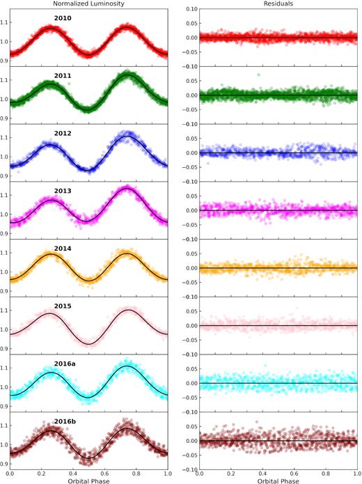
Left: optical light curves for all eight epochs of observations of CX137 phased at the photometric ephemeris. We include the best-fitting model described in Section 4.3 in black, where the luminosity of each epoch is divided by its average luminosity. Each panel shows a different epoch in order of time, error bars are not plotted since they are smaller than the data marker size. Right: fractional residuals of the best-fitting model to the light curve.
5 DISCUSSION
5.1 Stellar parameters
We calculate f for each model by measuring the relative flux fraction that the secondary contributes to the total flux of the system in the V band, the closest band to the 5580–6150 Å wavelength range used in Section 2.3 to derive f = 0.52 ± 0.06 from the spectroscopy. From the light-curve modelling, we find f-factors averaged over a full orbit for all epochs of photometry of: f = 0.50 ± 0.03 for the variable disc model, f = 0.54 ± 0.04 for the asymmetrical edge brightness model and f = 0.51 ± 0.09 for the spotted star model. Most of these are in perfect agreement with the value measured from the spectra. The f as a function of epoch is shown in Table 4.
We find best-fitting values for the primary mass of M1 = 0.81, 0.86, and 0.83 M⊙ for models 1, 2, and 3, respectively. The statistical uncertainties reported in Table 5 are in the order of the systematic uncertainties from assuming different models. Accounting for these, we adopt a primary mass estimate of M1 = 0.83 ± 0.06 M⊙, typical for white dwarfs in CVs (e.g. MWD = 0.83 ± 0.23 M⊙, Zorotovic, Schreiber & Gänsicke 2011), and too small for a neutron star (Özel & Freire 2016). The best estimate for the mass for the secondary is M2 = 0.65 ± 0.07 M⊙, consistent with the mass of a main-sequence K7 star (Cox 2000) and in agreement with the best-fitting template match found in Section 2.3. We find a best-fitting radius for the Roche Lobe of the secondary of R2 = 0.97 ± 0.15 R⊙. This radius is larger than expected for a main-sequence K7 star (which have typical values of R ∼ 0.65 R⊙, Pecaut & Mamajek 2013), supporting an evolved secondary in CX137.
Best-fitting parameters.
| Parameter | Prior | Variable disc | Asymmetrical brightness | Spotted secondary |
|---|---|---|---|---|
| i | cos ([0.0, 90]) | 63.8 ± 0.5 deg | 62.2 ± 0.2 deg | 63.1 ± 0.4 deg |
| T2 | [3500, 4100] | 4055 ± 25 K | 3850 ± 50 K | 4050 ± 30 K |
| q | 0.79 ± 0.06 | 0.767 ± 0.005 | 0.78 ± 0.01 | 0.779 ± 0.006 |
| vsin (i)* | 101 ± 3.0 | 99.5 ± 0.2 km s−1 | 100.6 ± 0.1 km s−1 | 100.5 ± 0.2 km s−1 |
| M1* | ⋅⋅⋅ | 0.81 ± 0.05 M⊙ | 0.86 ± 0.03 M⊙ | 0.83 ± 0.05 M⊙ |
| M2* | ⋅⋅⋅ | 0.62 ± 0.04 M⊙ | 0.68 ± 0.03 M⊙ | 0.65 ± 0.05 M⊙ |
| R2* | ⋅⋅⋅ | 0.92 ± 0.09 R⊙ | 1.02 ± 0.07 R⊙ | 0.97 ± 0.10 R⊙ |
Notes: list of the best-fitting parameters that are constant throughout all epochs of photometry and fit for in all models. i is the orbital inclination, T2 is the secondary temperature, q is the mass ratio, vsin (i) is the secondary’s rotational velocity, and M1 and M2 are the primary and secondary mass, respectively. And R2* is the radius of the Roche Lobe of the secondary. For most fit for parameters we adopt a flat prior, except for the orbital inclination, which is flat in cos (i), and the mass ratio, which has a Gaussian prior.
*These parameters were not fit for, but were calculated using all the posterior distribution samples of the fitted parameters.
From the spectra, we determine the ratio of the double-peak separation (DP) to the full width at half-maximum (FWHM) of the Hα emission line following the method of Casares (2016). We fit Hα with a double Gaussian function to measure the DP between the two line peaks DP = 484 ± 12 km s−1 and then fit a single Gaussian to determine the FWHM = 901 ± 19 km s−1. We find the average ratio to be DP/FWHM = 0.55 ± 0.02, the result of these fits are shown in Fig. 5. In Fig. 6, we show the q, and DP/FWHM of Hα plotted alongside the values for other known CVs. We confirm that our parameter estimates agree well with the q–DP/FWHM relation for CVs determined by Casares (2016). Torres et al. (2014) suggested the double-peaked structure of Hα might be due to contamination from photospheric absorption lines from the secondary (e.g. Torres et al. 2019). Nevertheless, the values we derived for CX137 agree with this trend, and strengthens the case that CX137 is a CV.
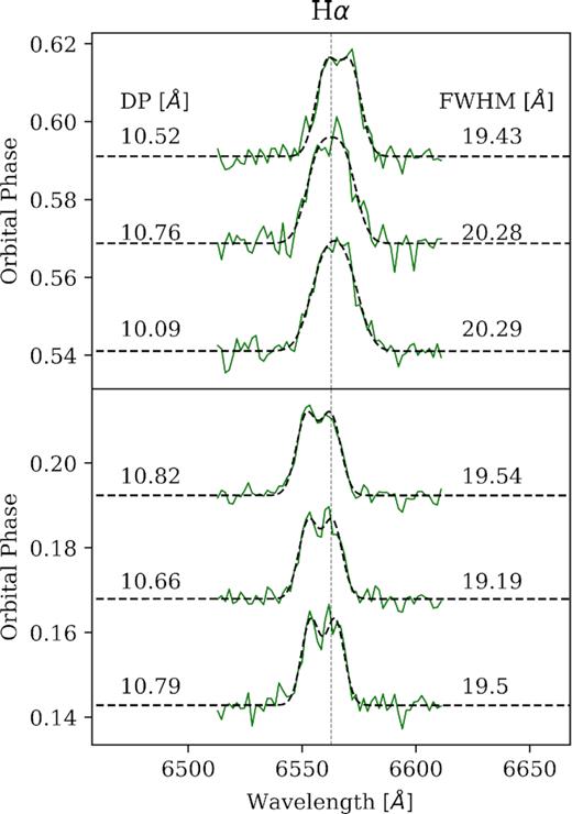
Emission-line profiles for Hα at 6 different phases. The best-fitting separation between the two peaks (DP) and the FWHM is shown in each panel. We determine a ratio of DP/FWHM = 0.55 ± 0.02 following the methods of Casares (2016).
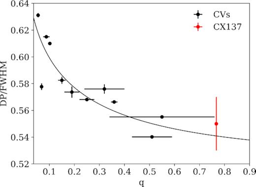
Relation between mass ratio q and ratio of peak separation DP to FWHM of Hα for known CVs. The black line is an empirical relation found in Casares (2016), from which this figure is adapted. The parameters found for CX137, shown in red, are consistent with the existing relations for CVs. Error bars not visible are smaller than the marker size.
Similarly, we calculate the expected FWHM of Hα using the FWHM–K2 relation for CVs from Casares (2015). A mass ratio q = 0.78 and an FWHM =936 ± 35 km s−1, corresponds to an expected value of K2 = 145 ± 22 km s−1, where the uncertainty is dominated by the scatter from the Casares relation. Consistent within the measured value of K2 = 161 ± 6 km s−1.
We measure the systemic velocity of CX137 from the optical spectra to be γ = 54 ± 4 km s−1 (Fig. 3). Given the proper motion and distance to CX137 obtained by Gaia (see Section 2.1), we can determine the space velocity of CX137 with respect to the Sun to be v = 62 ± 4 km s−1, statistically consistent with other CVs (v = 51 ± 7 km s−1; Ak et al. 2010).
In addition to the orbital period of the binary, we detect a tentative periodicity of ∼796 d. Stellar spots are known to live well over this amount of time and up to ∼10 yr (e.g, Hall & Henry 1994; Savanov 2014). As we saw in Model 3, it is possible that these long-term periodicity is produced by the evolution of spots on the surface of the secondary. Nevertheless, our photometry only covers a baseline three times that of this period, making its interpretation or physical origin hard to establish.
5.2 X-ray luminosity
Torres et al. (2014) provide a lower limit to the X-ray luminosity of CX137 of Lx > 5.8 × 1030 erg s−1 for a distance of 0.7 kpc and assuming a hydrogen column density NH = 1021 cm−2. Here, we improve this measurement by using the distance to CX137 from Gaia of |$d = 879^{+59}_{-52}$| pc (Bailer-Jones et al. 2018). In addition, we calculate the extinction in the line of sight to CX137 from the Bayestar19 3D dust maps (Green et al. 2019) to be AV ≈ 0.58. We obtain an NH = 1.7 × 1021 cm−2 from the AV–NH relation from Güver & Özel (2009). We calculate a counts to unabsorbed flux conversion ratio of 5.6 × 10⁻¹⁵ erg cm−2 s−1 count−1 for a 2.16 ks exposure taken with the Advanced CCD Imaging Spectrometer (ACIS-I) during Chandra Cycle 9, using a power-law spectrum with Γ = 2. This corresponds to a 0.5–10 keV unabsorbed flux of (8.4 ± 2.1) × 10−14 erg cm−2 s−1, or Lx = (7.8 ± 2.2) × 1030 erg s−1 at the distance from Gaia.
We can estimate an accretion rate following the method of Beuermann et al. (2004) using |$L_{\rm acc} = \dot{M} G M_1 (1/R_1 - 1/R_D)$|, R1 = (1.463 − 0.885(M1/M⊙)) × 109 cm, and Lacc = (1 + α)Lx; where α is typically 0.1. We adopt our best estimate for the primary mass of M1 = 0.83 M⊙, and a typical disc radius of RD = 1010 cm, as determined by our models presented in Section 4. We obtain an accretion rate estimate of |$\dot{M} \sim 10^{15}$| g s−1 (10−10.8 M⊙ yr−1).
Bahramian et al. (2020) detected CX137 at a higher Lx in the Swift Bulge Survey (Shaw et al. 2020) during repeated biweekly scans of the Galactic Bulge with the Neil Gehrels Swift Observatory. They measured an average Lx = 5 × 1031 erg s−1 over many epochs in 2017, with a peak of Lx = 3 ± 2 × 1032 erg s−1, indicating a flux increase of |$38^{+33}_{-26}$| compared to the Chandra GBS measurement, which would consequently bring up the accretion rate to |$\dot{M} \sim 4\times 10^{16}$| g s−1 (10−9.2 M⊙ yr−1) during this period. van Teeseling, Beuermann & Verbunt (1996) found that the accretion rate in non-magnetic CVs is likely underestimated by a factor of ∼2 for systems with inclinations of ≳ 60 deg. This would bring the accretion rate to |$\dot{M} \sim 10^{17}$| g s−1 (10−8.8 M⊙ yr−1), more similar to the |$\dot{M}$| expected for a Roche Lobe filling subgiant with an orbital period of 10 h (King, Kolb & Burderi 1996). An accretion rate of |$\dot{M} \sim 10^{17}$| g s−1 is expected for CVs with long periods ≳ 4 h, yet it is still low for a CV with a 10 h period like CX137 (Wynn, King & Horne 1997).
Using the Lx versus duty cycle correlation for dwarf novae from Britt et al. (2015), we can estimate the duty cycle for CX137 to be 0.063 ± 0.022. Accounting for observational cadence, the source should have been in outburst during 94 ± 34 d out of the 1504 days CX137 was observed by OGLE. One explanation for the lack of outbursts might be that CVs with long orbital periods tend to have shorter outbursts (Hameury & Lasota 2017). Given that the secondary star in CX137 contributes a large fraction of the total flux, an outburst would be of low amplitude, and we could have missed it if it happened when the source was not being observed. KIC 5608384 is another example of a CV with a long period (8.7 h) and a low accretion rate (|$\dot{M} = 0.3 - 6.5 \times 10^{-9}$| M⊙ yr−1) that showed only one 4 d outburst in four years of Kepler photometry (Yu et al. 2019).
6 CONCLUSION
We obtained multiple spectra of the binary star CX137 and constructed a radial velocity curve from which we measure a K2 = 161.1 ± 0.7 km s−1 and a systemic velocity γ = 54 ± 4 km s−1. Additionally, we modelled 7 yr of optical photometry. The optical light curve has an asymmetrical sine curve shape, which we interpret as being due to ellipsoidal modulations of a tidally distorted secondary star. We see long-term variations in the shape of the light curve, which are well fitted by a spotted secondary star (Model 3; Section 4.3). From the light-curve modelling, we derive a best-fitting inclination of i = 63.0 ± 0.7 deg, a primary mass of M1 = 0.83 ± 0.06 M⊙, consistent with a white dwarf accretor, and a secondary mass of M2 = 0.65 ± 0.07 M⊙, consistent with an evolved K7 secondary.
SUPPORTING INFORMATION
CX137_Photometry.txt
Please note: Oxford University Press is not responsible for the content or functionality of any supporting materials supplied by the authors. Any queries (other than missing material) should be directed to the corresponding author for the article.
ACKNOWLEDGEMENTS
This project was supported in part by an NSF GROW fellowship. PGJ and ZKR acknowledge funding from the European Research Council under ERC Consolidator grant agreement no. 647208. JS was supported by a Packard Fellowship. MAPT acknowledge support by the Spanish MINECO under grant AYA2017-83216-P and support via Ramón y Cajal Fellowship RYC-2015-17854. We thank Tom Marsh for the use of molly. This work has made use of data from the European Space Agency (ESA) mission Gaia (https://www.cosmos.esa.int/gaia), processed by the Gaia Data Processing and Analysis Consortium (DPAC, https://www.cosmos.esa.int/web/gaia/dpac/consortium). Funding for the DPAC has been provided by National Institutions, in particular the institutions participating in the Gaia Multilateral Agreement. The ISIS spectroscopy was obtained with the WHT, operated on the island of La Palma by the Isaac Newton Group of Telescopes in the Spanish Observatorio del Roque de los Muchachos of the Instituto de Astrofisica de Canarias. This paper includes data gathered with the 6.5 m Magellan Telescopes located at Las Campanas Observatory, Chile. This research has made use of NASA’s Astrophysics Data System. This research has made use of the SIMBAD database, operated at CDS, Strasbourg, France. The OGLE project has received funding from the National Science Centre, Poland, grant MAESTRO 2014/14/A/ST9/00121 to AU.
Software:astropy (Astropy Collaboration et al. 2018), pyraf (Science Software Branch at STScI 2012), SAOImage DS9 (Smithsonian Astrophysical Observatory 2000), emcee (Foreman-Mackey et al. 2013), corner (Foreman-Mackey 2016), matplotlib (Hunter 2007), scipy (van der Walt, Colbert & Varoquaux 2011), numpy (Oliphant 2007), extinction (Barbary 2016), pyphot (https://github.com/mfouesneau/pyphot), molly (http://deneb.astro.warwick.ac.uk/phsaap/software/molly/html/INDEX.html), and xrbinary(http://www.as.utexas.edu/∼elr/Robinson/XRbinary.pdf).
DATA AVAILABILITY
All the optical photometry used for this work are available on the online Supporting Information version of this article. And the radial velocity data is shown in Table A1.
Footnotes
iraf is written and supported by the National Optical Astronomy Observatories, operated by the Association of Universities for Research in Astronomy, Inc. under cooperative agreement with the National Science Foundation.
molly is a code developed and maintained by Marsh and it is available at http://deneb.astro.warwick.ac.uk/phsaap/software/molly/html/INDEX.html
A full description of xrbinary can be found at http://www.as.utexas.edu/∼elr/Robinson/XRbinary.pdf
REFERENCES
APPENDIX A: RADIAL VELOCITY TABLE
This section contains a data table with all the relevant radial velocity measurements.
Radial velocity measurements.
| HJD | Phase | Blue arm | Red arm |
|---|---|---|---|
| (km s−1) | (km s−1) | ||
| 2457928.59333808 | 0.12 ± 0.01 | 147.58 ± 17.02 | 176.82 ± 32.42 |
| 2457928.60054154 | 0.14 ± 0.01 | 165.92 ± 17.87 | 174.49 ± 43.66 |
| 2457928.61416582 | 0.17 ± 0.01 | 188.48 ± 15.63 | 204.0 ± 41.87 |
| 2457928.62136939 | 0.19 ± 0.01 | 191.22 ± 15.28 | 229.08 ± 46.91 |
| 2457928.63017967 | 0.21 ± 0.007 | 279.04 ± 35.36 | 173.87 ± 23.30 |
| 2457928.63866717 | 0.23 ± 0.007 | 269.75 ± 34.11 | ⋅⋅⋅ |
| 2457945.52058442 | 0.26 ± 0.007 | 179.98 ± 34.33 | 143.12 ± 22.97 |
| 2457945.52778765 | 0.28 ± 0.007 | 138.03 ± 7.03 | 170.52 ± 10.81 |
| 2457945.53499120 | 0.30 ± 0.007 | 325.63 ± 35.34 | 173.73 ± 8.88 |
| 2457945.54556637 | 0.32 ± 0.007 | 296.82 ± 25.86 | 176.81 ± 14.35 |
| 2457945.55276959 | 0.48 ± 0.007 | 51.32 ± 18.00 | 88.6 ± 20.27 |
| 2457945.55997296 | 0.50 ± 0.007 | 41.01 ± 19.48 | 36.56 ± 22.01 |
| 2457955.53460348 | 0.51 ± 0.007 | −10.06 ± 20.93 | 77.07 ± 22.96 |
| 2457955.54538190 | 0.54 ± 0.007 | −51.22 ± 19.54 | 61.0 ± 21.58 |
| 2457955.55613857 | 0.56 ± 0.01 | −32.42 ± 19.73 | 77.23 ± 19.12 |
| 2457955.56690152 | 0.57 ± 0.007 | −65.28 ± 21.94 | −9.73 ± 17.04 |
| 2457955.57773804 | 0.71 ± 0.007 | −115.45 ± 17.05 | −95.98 ± 11.91 |
| 2457956.39406596 | 0.74 ± 0.01 | −103.73 ± 16.63 | −107.96 ± 12.11 |
| 2457956.40482062 | 0.76 ± 0.01 | −102.91 ± 17.06 | −100.52 ± 11.31 |
| 2457956.41896960 | 0.79 ± 0.01 | −107.86 ± 16.42 | −93.96 ± 10.07 |
| 2457956.42972824 | 0.81 ± 0.01 | −90.24 ± 17.58 | −83.48 ± 12.03 |
| 2457956.44047118 | 0.71 ± 0.01 | −118.98 ± 15.49 | −91.92 ± 12.57 |
| 2457956.45125232 | 0.73 ± 0.01 | −129.45 ± 16.73 | −95.19 ± 11.78 |
| 2457956.46203540 | 0.77 ± 0.01 | −107.13 ± 16.41 | −105.07 ± 10.57 |
| 2457956.47942908 | 0.79 ± 0.01 | −114.13 ± 16.48 | −115.54 ± 12.78 |
| 2457956.49018300 | 0.82 ± 0.01 | −82.39 ± 14.79 | −61.39 ± 15.10 |
| 2457956.50090890 | 0.84 ± 0.01 | −83.39 ± 14.81 | −73.31 ± 11.55 |
| 2457993.39230059 | 0.87 ± 0.01 | −67.96 ± 15.32 | −85.09 ± 11.04 |
| 2457993.40297597 | 0.91 ± 0.01 | −25.48 ± 15.72 | −35.57 ± 10.69 |
| 2457993.41365122 | 0.93 ± 0.01 | −29.25 ± 15.76 | 18.58 ± 12.15 |
| 2457995.36471471 | 0.96 ± 0.01 | 3.35 ± 18.52 | 37.29 ± 12.94 |
| 2457995.37539082 | 0.54 ± 0.01 | −5.51 ± 19.23 | −10.56 ± 42.03 |
| 2457995.38606633 | 0.57 ± 0.01 | −30.79 ± 20.13 | 50.13 ± 56.59 |
| 2457995.39677799 | 0.59 ± 0.01 | −44.82 ± 18.25 | −46.38 ± 41.77 |
Notes: radial velocity measurements shown in Fig. 3 taken simultaneously with the red and blue arms of the ISIS spectrograph. Corrected for heliocentric velocity.
