


ABSTRACT
In this work, we study the shape of the projected surface mass density distribution of galaxy clusters using weak-lensing stacking techniques. In particular, we constrain the average aligned component of the projected ellipticity, ϵ, for a sample of redMaPPer clusters (0.1 ≤ z < 0.4). We consider six different proxies for the cluster orientation and measure ϵ for three ranges of projected distances from the cluster centres. The mass distribution in the inner region (up to 700 kpc) is better traced by the cluster galaxies with a higher membership probability, while the outer region (from 700 kpc up to 5 Mpc) is better traced by the inclusion of less probable galaxy cluster members. The fitted ellipticity in the inner region is ϵ = 0.21 ± 0.04, in agreement with previous estimates. We also study the relation between ϵ and the cluster mean redshift and richness. By splitting the sample in two redshift ranges according to the median redshift, we obtain larger ϵ values for clusters at higher redshifts, consistent with the expectation from simulations. In addition, we obtain higher ellipticity values in the outer region of clusters at low redshifts. We discuss several systematic effects that might affect the measured lensing ellipticities and their relation to the derived ellipticity of the mass distribution.
1 INTRODUCTION
According to the current Lambda cold dark matter (ΛCDM) cosmological paradigm, structures in the Universe are formed hierarchically from gravitational collapse due to initial density fluctuations (Kravtsov & Borgani 2012). As matter collapses, gas condensation results on star formation and eventual galaxy formation occur within these matter overdensities. Therefore, galaxies and galaxy systems are expected to reside on highly overdense dark matter clumps of increasing mass, named as dark matter haloes. In this scenario, massive haloes are formed from the accretion of smaller ones. These low-mass haloes are accreted in preferential directions, mainly along the filamentary distribution. Therefore, dark matter haloes are not expected to have spherical shapes. In fact, studies of dark matter haloes in numerical simulations have shown that halo shapes can be well described by a triaxial model with a tendency of being prolate (Dubinski & Carlberg 1991; Warren et al. 1992; Cole & Lacey 1996; Jing & Suto 2002; Bailin & Steinmetz 2005; Hopkins, Bahcall & Bode 2005; Kasun & Evrard 2005; Allgood et al. 2006; Paz et al. 2006; Bett et al. 2007; Muñoz-Cuartas et al. 2011; Schneider, Frenk & Cole 2012; Despali, Tormen & Sheth 2013; Velliscig et al. 2015; Vega-Ferrero, Yepes & Gottlöber 2017).
Numerical simulations also predict that more massive haloes tend to be less spherical since they are formed later, thus, they are less dynamically relaxed. The same is expected for haloes at larger redshifts (Jing & Suto 2002; Allgood et al. 2006; Muñoz-Cuartas et al. 2011; Velliscig et al. 2015), because they are affected by the direction of the last major merger and the presence of filaments around them (Bonamigo et al. 2015). Clusters of galaxies appear to be less spherical towards their centres in dark matter only simulations (Warren et al. 1992; Jing & Suto 2002; Bailin & Steinmetz 2005; Allgood et al. 2006; Schneider et al. 2012). This last trend is less significant when baryonic effects are incorporated, i.e. the dark matter distribution becomes more spherical in the inner regions due to the baryon effect (Velliscig et al. 2015; Suto et al. 2017; Chua et al. 2019). Moreover, the trend is reversed when self-interacting dark matter is considered and the halo becomes rounder towards the centre as the considered cross-section of the dark matter particle increases (Robertson et al. 2019).
Gravitational lensing provides a unique technique to constrain the mean projected halo ellipticity. A triaxial dark matter halo will produce an azimuthal variation of the lensing signal, causing a larger amplitude of the observed signal along the projected major axis direction. This effect can be well modelled to obtain the projected ellipticity for individual targets as long as massive galaxy clusters or deep data are considered (e.g. Oguri et al. 2010, 2012; Chiu et al. 2018; Umetsu et al. 2018; Harvey et al. 2019; Okabe et al. 2020). Nevertheless, when lower mass haloes are analysed, constraining the lensing signal is a hard task. In the weak-lensing regime, the combination of a large sample of systems is needed to obtain a reliable determination of the halo ellipticity, known as stacking techniques (Brainerd & Wright 2000; Natarajan & Refregier 2000). Another difficulty comes from the necessity of making assumptions regarding the projected major semi-axis orientation in order to align the systems. Misalignment between the adopted angle and the true halo orientation would result in a depletion of the detected signal, thus underestimating the halo ellipticity.
In spite of these difficulties, several studies were able to successfully measure the projected halo ellipticity using weak-lensing techniques for a wide range of masses. For galaxy scale haloes, assuming that the galaxy and the halo are aligned, the average ratio between the aligned component of the halo ellipticity and the ellipticity of the light distribution could be successfully constrained (Mandelbaum et al. 2006; Parker et al. 2007; van Uitert et al. 2012; Schrabback et al. 2015, 2020). For the group- and cluster-scale, either the major semi-axis of the brightest cluster (or group) galaxy member (BCG), or the distribution of the galaxy members, have been used as proxies to trace the halo orientation. While the BCG’s major axis is the optimal proxy to trace the matter orientation on small scales (≲250 kpc; van Uitert et al. 2017), the member distribution is better aligned with the matter at the outskirts of the galaxy systems. Using this approach, the mean projected halo ellipticity for these systems has been successfully estimated, obtaining an aligned component of ∼0.2–0.5 (Evans & Bridle 2009; Oguri et al. 2010; Clampitt & Jain 2016; van Uitert et al. 2017; Shin et al. 2018).
In this work, we present the analysis of the aligned component of the projected surface mass ellipticity for SDSS redMaPPer clusters (Rykoff et al. 2014) using weak-lensing stacking techniques. For this sake, we take advantage of high-quality public weak-lensing surveys, combining these data to increase the signal to noise of our measurements. In order to align the combined clusters, we estimate the surface density orientation angle of each galaxy cluster taking into account the satellite1 distribution. We define different proxies to estimate this orientation, considering different weights and cuts for the satellite galaxies that are assumed to trace the mass distribution. Given the high-mass systems considered for the analysis and the good-quality data used to obtain the lensing signal, we also study the relation between the derived projected ellipticity and the average cluster mass and redshift. Furthermore, we analyse the projected lensing signal at different ranges of distances from the cluster centres to obtain information about the orientation of the surface mass density distribution at the inner and outer parts of the clusters. The main motivation is to study the halo ellipticity as well as the orientation of the surface mass distribution at the outskirts of the cluster.
This paper is organized as follow: In Section 2, we describe the data used in this work, the weak-lensing catalogues and the sample of clusters. We describe how the projected matter orientation is estimated for each cluster in Section 3. In Section 4, we describe the lensing analysis applied in order to derive the aligned component of the projected ellipticity. We present our results in Section 5 and discuss different sources of biases in Section 6. Finally, we discuss our results in Section 7 and conclude in Section 8. We adopt when necessary a standard cosmological model with H0 = 70h70 km s−1 Mpc−1, Ωm = 0.3, and ΩΛ = 0.7.
2 OBSERVATIONAL DATA
2.1 Weak-lensing surveys
In order to perform the weak-lensing analysis we combine the catalogues from four public weak-lensing surveys. All the combined data (except for KiDS-450) are based on imaging surveys carried-out using the MegaCam camera (Boulade et al. 2003) mounted on the Canada–France–Hawaii Telescope (CFHT), thus having similar image quality. Data products were combined using theli (Erben et al. 2013). Although KiDS-450 shear catalogue is based on observations obtained with a different camera, both cameras share similar properties, such as a pixel scale of 0.2 arcsec. Also, the seeing conditions are similar for all the surveys (∼0.6 arcsec). Moreover, all the source galaxy catalogues were obtained using lensfit (Miller et al. 2007; Kitching et al. 2008) to compute the shape measurements and photometric redshifts are estimated using the BPZ algorithm (Benítez 2000; Coe et al. 2006). For the analysis we applied the additive calibration correction factors for the ellipticity components provided for each catalogue. We also apply a multiplicative shear calibration factor to the combined sample of galaxies as suggested by Miller et al. (2013) (see Section 4.3). In the next subsections we will briefly describe the shear catalogues used.
From the weak-lensing catalogues, we select the galaxies for the lensing study by applying the following cuts to the lensfit parameters: MASK ≤ 1, FITCLASS = 0, and w > 0. Here, MASK is a masking flag, FITCLASS is a flag parameter given by lensfit which takes the value 0 when the source is classified as a galaxy, and w is a weight parameter that takes into account errors on the shape measurement and the intrinsic shape noise, which ensures that galaxies have well-measured shapes (see details in Miller et al. 2013). Background galaxies, defined as the galaxies that are located behind the galaxy clusters and thus affected by the lensing effect, are selected taking into account the photometric redshift information with a similar criteria as the one used in previous studies (e.g. Leauthaud et al. 2017; Chalela et al. 2018; Pereira et al. 2018; Gonzalez et al. 2019). We consider a galaxy as a background galaxy if it satisfies Z_BEST > zc + 0.1 and ODDS_BEST > 0.5, where Z_BEST is the photometric redshift estimated for each galaxy, zc is the considered cluster redshift, and ODDS_BEST is a parameter that expresses the quality of Z_BEST and takes values from 0 to 1. We neglect the effect of the inclusion of foreground and/or cluster galaxies in the background sample, known as ‘boost factor’, which cause a dilution effect in the lensing signal, since it is expected to be negligible considering the cuts implemented in the background sample selection (Blake et al. 2016; Leauthaud et al. 2017; Shan et al. 2018). To assign background galaxies to each galaxy cluster we use the public regular grid search algorithm grispy2 (Chalela et al. 2019). An analysis of the lensing signal computed for the individual catalogues is presented in Appendix A as a control test for their combination.
2.1.1 CFHTLens
The Canada–France–Hawaii Telescope Lensing Survey (CFHTLenS) weak-lensing catalogues3 are based on the data collected as part of the CFHT Legacy Survey. This is a multiband survey (u*g′r′i′z′) that spans 154 deg2 distributed in four separate patches W1, W2, W3, and W4 (63.8, 22.6, 44.2, and 23.3 deg2, respectively). The achieved limiting magnitude is i′ ∼ 25.5 considering a 5σ point source detection. Further details regarding image reduction, shape measurements, and photometric redshifts can be found in Hildebrandt et al. (2012), Heymans et al. (2012), Miller et al. (2013), and Erben et al. (2013). The shear catalogue is based on the i-band measurements, achieving a weighted galaxy source density of ∼15.1 arcmin−2.
2.1.2 CS82
The CS82 shear catalogue is based on the CFHT Stripe 82 survey, a joint Canada–France–Brazil project designed with the goal of complementing existing SDSS Stripe 82 ugriz photometry with high-quality i-band imaging suitable for weak and strong lensing measurements (e.g. Shan et al. 2014; Hand et al. 2015; Liu et al. 2015; Bundy et al. 2017; Leauthaud et al. 2017; Niemiec et al. 2017; Shan et al. 2017; Pereira et al. 2018). This survey spans over a window of 2 × 85 deg2, with an effective area of 129.2 deg2, after masking out bright stars and other image artefacts. It has a median point spread function (PSF) of 0.6 arcsec and a limiting magnitude i′ ∼ 24 (Leauthaud et al. 2017). The source galaxy catalogue has an effective weighted galaxy number density of ∼12.3 arcmin−2.
2.1.3 RCSLens
The RCSLens catalogue4 (Hildebrandt et al. 2016) is based on the Red-sequence Cluster Survey 2 (RCS-2; Gilbank et al. 2011), a multiband imaging survey in the griz bands with a depth of ∼24.3 in the r band, considering a point source at 7σ detection level. The survey spans over ∼785 deg2 distributed in 14 patches, the largest being 10 × 10 deg2 and the smallest 6 × 6 deg2. The source catalogue based on the r-band imaging, achieves an effective weighted galaxy number density of ∼5.5 arcmin−2. A full systematic error analysis of the shear measurements in combination with the photometric redshifts is presented in Hildebrandt et al. (2016), with additional error analyses of the photometric redshift measurements presented in Choi et al. (2016).
2.1.4 KiDS-450
The KiDS-450 catalogue5 (Hildebrandt et al. 2017) is based on the third data release of the Kilo Degree Survey (KiDS; Kuijken et al. 2015) which spans over 447 deg2. This is a multiband imaging survey (ugri) carried out with the Omega-CAM CCD mosaic camera mounted on the VLT Survey Telescope. Shear catalogues are based on the r-band images with a mean PSF of 0.68 arcsec and a 5σ limiting magnitude of 25.0. Shape measurements are performed using an upgraded version of lensfit algorithm (Fenech Conti et al. 2017). The resultant source catalogue has an effective weighted galaxy number density of ∼8.53 arcmin−2.
2.2 redMaPPer clusters
The full sample consists of 26 111 clusters with richness 20 ≲ λ < 300 spanning a redshift range of 0.08 ≲ zc < 0.6. For this work we restrict our sample to 20 ≤ λ < 150 and 0.1 ≤ zc < 0.4. The upper limit in the redshift selection is performed considering our weak-lensing data and because up to this redshift the number of galaxies lost due to the SDSS depth is relatively small. We also discard the clusters at the edges of the SDSS field, in order to avoid clusters with missing cluster members due to border issues. Therefore, we kept only the clusters that lie at more than 2 Mpc from the border of the SDSS sky coverage. Finally, we only include the clusters located within the regions of the weak-lensing data described previously, using the data from the deepest lensing catalogue in the case of overlapping areas. The total cluster sample used in this work includes 2 275 clusters. We show in Fig. 1 the distribution of richness and redshifts of these clusters. To study the relation between the projected ellipticity and the mass and redshift of the halo, we split our total sample in four roughly equally number samples according to the median redshift (z = 0.313) and richness (λ = 27.982) of the sample.
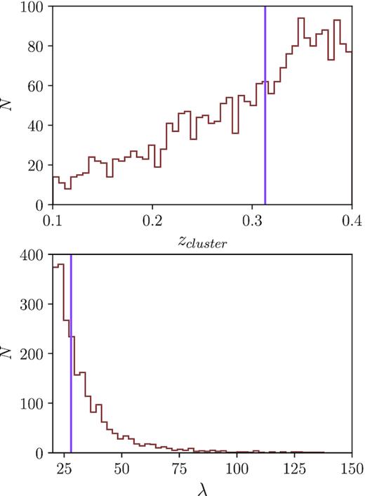
Distribution of redshifts (upper panel) and richness (lower panel) of the redMaPPer clusters used in this work. The vertical lines correspond to the median values of these parameters.
3 ESTIMATING THE SURFACE DENSITY ORIENTATION
To get an insight on which member galaxies trace better the mass distribution, we consider different criteria to compute the quadrupole moments. For the weights we consider three types: (1) a uniform weight, wk = 1; (2) according to the r-band luminosity, wk = Lk, and (3) according to the projected distance from the centre, |$w_k = 1/(x^2_{1,k} + x^2_{2,k})$|. We also take into account for the computation all the galaxy members in the sample and only those with a membership probability larger than 0.5 (pmem > 0.5). According to the different criteria adopted to compute the quadrupole moments, we use in total six different proxies to estimate the orientation angle for each cluster, named as ϕ1, ϕL, ϕd, when considering the total sample of satellites with an uniform weight, a luminosity weight, and a distance weight, respectively, and |$\phi ^*_1$|, |$\phi ^*_L$|, |$\phi ^*_d$| when considering only the satellites with pmem > 0.5 and the respective weights. The membership probability cut applied to select the satellites, lowers the number of interlopers that could result in an underestimated ellipticity measurement (Shin et al. 2018), i.e. lowers the number of foreground and background galaxies that were wrongly classified as cluster members. Nevertheless, since this parameter strongly depends on the distance to the cluster centre, it can filter the satellites that lie on the outskirt of the cluster.
In Fig. 2, we show the number density contours of all the satellites stacked along the different orientations defined above, considering the projected coordinates re-scaled according to the radius cluster, Rλ. In Fig. 3, we show the distribution of distances to the adopted cluster centre for the satellites, derived weighting the distances according to the weights defined above, for the total sample of satellites and those with pmem > 0.5. As it can be noticed, when the distance weight is considered, the derived orientation angle follows the distribution of the satellites that are located at the inner regions of the cluster. Also, as expected, when we consider only the satellites with pmem > 0.5, the distance distribution tend to lower values. In Table 1, we show the estimated raw ellipticity values. Although with a high dispersion, larger values are derived when considering a luminosity weight and only satellites with pmem > 0.5 to compute the quadrupole moments. Distribution of the differences between the orientation angles considering the defined weights and the membership cut have a standard deviation of ∼45–55 deg.
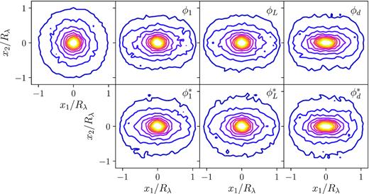
Satellite number density contours for the sample of redMaPPer clusters used in this work, obtained by stacking the galaxies aligned according to the estimated orientation angle. Projected positions, x1 and x2, are re-scaled with the cluster radius, Rλ. The first panel at the left was obtained without aligning the clusters. First row of panels is obtained considering all the satellites in the catalogue and the second row discarding the galaxies with pmem < 0.5 to estimate the orientation angle. Second, third, and fourth columns correspond to the orientation computed considering a uniform, a luminosity, and a distance weight to compute the quadrupole moments, respectively.
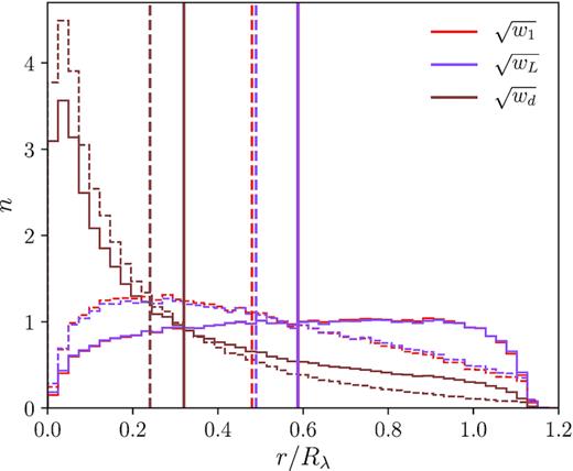
Normalized distributions of distances to the centre for the satellite galaxies, obtained by weighting the distances according to the square root of the defined uniform (red line), luminosity (purple line), and distance (brown line) weights. Dashed lines correspond to the distribution of satellites that satisfy pmem > 0.5. Vertical lines show the average weighted values for these distributions. Distributions for the total sample of satellites considering the uniform and luminosity weights are almost coincident therefore the mean values are overlapped.
Mean raw ellipticity (〈ϵ〉) and standard deviation (σϵ) estimates for the sample of clusters, derived according to the quadrupole moments taking into account different samples of satellites and weights (wk).
| Orientation | Satellite sample | wk | 〈ϵsat〉 | σϵ |
|---|---|---|---|---|
| ϕ1 | Total | 1 | 0.21 | 0.11 |
| ϕL | Total | Lk | 0.26 | 0.13 |
| ϕd | Total | |$\big(x^2_{1,k} + x^2_{2,k}\big)^{-1}$| | 0.18 | 0.09 |
| |$\phi ^*_1$| | pmem > 0.5 | 1 | 0.29 | 0.15 |
| |$\phi ^*_L$| | pmem > 0.5 | Lk | 0.35 | 0.17 |
| |$\phi ^*_d$| | pmem > 0.5 | |$\big(x^2_{1,k} + x^2_{2,k}\big)^{-1}$| | 0.22 | 0.11 |
The satellite distribution has been used to estimate the halo ellipticity in previous works (Brainerd 2005; Bailin et al. 2008; Shin et al. 2018). As pointed out by Shin et al. (2018), ellipticity measurements derived from the satellite distribution are affected by a noise bias, introduced by the fact that a finite number of satellites is considered; an edge bias, since members are selected within a circular aperture and a bias introduced by the inclusion of interlopers, foreground or background red galaxies considered as members. In this work, we do not intend to measure the halo ellipticity from the satellite distribution but to use them as a proxy for the surface density orientation. Nevertheless, it is important to take into account that all the mentioned biases can impact on the estimation of the orientation angle. These issues will be discussed in more detail in Section 6.
4 WEAK-LENSING ANALYSIS
The weak gravitational lensing effect introduces a distortion in the luminous sources that are behind a gravitational potential considered as the lens. Galaxy systems in particular are powerful lenses that distort the shape of the galaxies that are behind, inducing an alignment of their shapes along the direction tangential to the lens mass distribution (Bartelmann, King & Schneider 2001). This distortion can be quantified by the complex-value lensing shear, γ = γ1 + iγ2, which can be estimated according to the measured ellipticity of the background galaxies, i.e. the galaxies that lie behind the galaxy cluster and thus, that are affected by the lensing effect. Since galaxies have their own intrinsic ellipticity, the observed source shape results in a combination of their intrinsic ellipticity and the ellipticity introduced by the lensing effect. Assuming that the galaxies are randomly orientated in the sky (for a large sample of galaxies at a wide range of distances from the lens), the shear can be estimated by averaging the ellipticity of many sources, 〈e〉 = γ, where the noise of this estimate scales with the number of sources (NS) considered in the average as |$1/\sqrt{N_\mathrm{ S}}$|.
In order to reduce the noise introduced by the intrinsic shape of the considered sources we use stacking techniques that consist on combining several lenses which artificially increase the density of sources. Stacking techniques can provide a lensing signal with a suitable confidence level which allow to derive the average projected density distribution of the combined lenses (e.g. Foëx et al. 2014; Leauthaud et al. 2017; Simet et al. 2017; Chalela et al. 2018; Pereira et al. 2018). Usually, galaxy clusters are stacked without considering a particular orientation therefore the derived radial density profiles can be well fitted using axisymmetric density mass distribution models.
In this section, we first describe how the monopole is modelled to derive the total masses of the considered cluster samples (Section 4.1). Then, we fit the ϵ considering the quadrupole modelling described in Section 4.2. To estimate the monopole and quadrupole components we combine the shape measurements of the background galaxy sample according to the estimators defined in Section 4.3
4.1 Isotropic lens model
On the other hand, the averaged cross component of the shear, γ×, defined as the component tilted at π/4 relative to the tangential component, should be zero. This quantity is therefore commonly used as a null test to check for the presence of systematics in the data.
When averaging the tangential component within an annulus, the anisotropic components of the surface density are vanished and only the monopole information is left (see Section 4.2). To derive the total masses of the considered cluster sample, we model the monopole component taking into account two terms: a perfectly centred dark matter halo profile and a miscentring term. The second term considers the offset between the redMaPPer centre and their host dark matter halo. This modelling is motivated by the fact that we do not know the true location of the halo centre and an observationally motivated centre is adopted. This results in an offset distribution that can be modelled with two populations, a miscentred group and a well-centred group. According to hydrodynamic simulations, when galactic centres are adopted the well-centred group could include up to about |$60{{\ \rm per\ cent}}$| of all the clusters (Yan et al. 2020).
To estimate the masses we fit the adopted model with two free parameters, pcc and M200. We fix the width of the offset distribution in equation (9), σoff = 0.4h−1Mpc, according to the result presented in Simet et al. (2017). We do not take into account a point mass term for a possible stellar- mass contribution of the central galaxies and a so-called 2-halo term due to neighbouring haloes. In order to avoid their contributions to the computed profiles, we fit the profiles from |$100 h_{70}^{-1}$| kpc up to |$5 h_{70}^{-1}$| Mpc, were these terms are not expected to have a significant impact for the mass estimates (Mandelbaum et al. 2006; Simet et al. 2017; Pereira et al. 2018).
4.2 Anisotropic lens model
4.3 Estimators and fitting procedure
In order to obtain the monopole and quadrupole profiles, we use a stacking procedure by combining the shape measurements of all the background galaxies selected for each sample of clusters, artificially increasing the number density of background galaxies and lowering the noise introduced by their intrinsic shapes.
The parameters that are fitted from the defined estimators are the logarithmic mass, log (M200), the fraction of miscentring clusters, pcc and the average aligned ellipticity component, ϵ. Our procedure consists of fitting log (M200) and pcc, considering only the monopole component (ΔΣ(r), see equation 12) according to the modelling presented in Section 4.1. Then, taking into account the estimated M200 we constrain ϵ by simultaneously fitting the quadrupole components, |$\Gamma _{\rm {t} \cos {2\theta }}(r)$| and Γ× sin 2θ(r). To model the anisotropic contribution of the shear-field included in the quadrupole components, we neglect the miscentring term, in spite it is considered to derive the halo masses by fitting the density contrast profile (equation 12). A wrong determination of the halo centre, as it is expected for |$\sim \! 20 {{\ \rm per\ cent}}$| of the redMaPPer clusters, can lead to underestimated lensing masses up to |$30{{\ \rm per\ cent}}$|, which would result in an overestimation of the projected ellipticities in |$\sim \! 25 {{\ \rm per\ cent}}$|. Nevertheless, we do not expect a significant contribution of this term in the quadrupole component as previously reported by other studies (van Uitert et al. 2017; Shin et al. 2018).
We constrain our free parameters by using the Markov chain Monte Carlo method, implemented through emcee python package (Foreman-Mackey et al. 2013), to optimize the log-likelihood functions for the monopole profile, |$\ln {\mathcal {L}}(\Delta \Sigma | r ,M_{200},p_{\mathrm{ cc}})$| and for the quadrupoles, |$\ln {\mathcal {L}}(\Gamma _{\rm {t} \cos {2\theta }} | r ,\epsilon) + \ln {\mathcal {L}}(\Gamma _{\times \sin {2\theta }} | r ,\epsilon)$|. To fit the data we use 10 chains for each parameter and 200 steps, considering flat priors for log (M200) and ϵ, (|$12.5 \lt \log (M_{200}/(h^{-1}_{70} M_\odot)) \lt 15.5$| and 0.0 < ϵ < 0.5) and for pcc we take into account the results from the X-ray observations (Rozo & Rykoff 2014) and consider as a prior a Gaussian distribution with a mean value of 0.8 and a standard deviation of 0.3. Our best-fitting parameters are obtained according to the median of the posterior distributions and errors are based on the differences between the median and the 16th and 84th percentiles, after discarding the first 50 steps of each chain.
In order to obtain information of the projected ellipticities at different radial distances, quadrupole profiles are fitted within three ranges: |$0.1 \lt r/(h^{-1}_{70}$| Mpc) < 5, |$0.1 \lt r/(h^{-1}_{70}$| Mpc) < 0.7, and |$0.7 \lt r/(h^{-1}_{70}$| Mpc) < 5. We refer to these ranges as |$r_{0.1}^{5.0}$|, |$r_{0.1}^{0.7}$|, and |$r_{0.7}^{5.0}$|, respectively. The selection cut at |$700\, h^{-1}_{70}$| kpc was made to have the same number of estimates in the inner and outer regions (five points each). We expect that the constrained ϵ within |$r_{0.1}^{0.7}$| to be more related to the projected density distribution at the inner regions of the clusters, thus, with the dark matter halo elongation. We note, however, that the shear quadrupole is not a direct measure of the ellipticity within a given radius, since the shear is related non-locally to the mass distribution. Therefore, if the ellipticity is a function of the radius, the quadrupole profiles (equations 22 and 23) will not yield the ellipticity at a projected distance r. Nevertheless, the ellipticity of the local mass distribution will contribute to the quadrupole. Hence, we will still use the value of ϵ derived from the quadrupole as an estimate of the elongation of the mass distribution at different radii.
We show as an example in Fig. 4, the computed monopole and quadrupole components for the total sample of redMaPPer, fitted within the whole projected distance range (|$r_{0.1}^{5.0}$|). The quadrupoles were obtained by considering ϕ1 as the proxy to estimate the orientation angle for the surface density distribution. The remaining fitted quadrupole components derived for all the estimated orientations and all the considered cluster samples are shown in Appendix B.
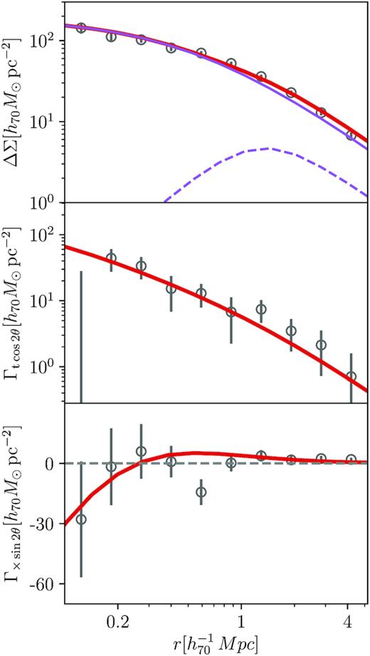
Monopole (upper panel) and quadrupole tangential (middle panel) and cross (bottom panel) components, computed for the total sample of clusters analysed in this work. Solid thick lines are the derived models according to the fitted mass, M200, and fraction of miscentring clusters, pcc, for the monopole, and the average aligned ellipticity component, ϵ, for the quadrupole components. In the upper panel, we also show both fitted terms for the monopole, the centred ΔΣcen (solid purple line), and the miscentring term, ΔΣmiss (dashed purple line), terms (see equation 12).
5 RESULTS
We obtained the average aligned ellipticity components for the five samples of redMaPPer clusters (total, high- and low-redshift, high- and low-richness samples) by fitting both quadrupole component profiles in the mentioned projected distance ranges. In order to obtain the quadrupole profiles, we compute θ for each source considering the halo orientations derived for each cluster, ϕ (equation 4), taking into account the proxies defined in Section 3 (|$\phi _1,\phi _L,\phi _d,\phi ^*_1,\phi ^*_L$|, and |$\phi ^*_d$|). We also compute a control quadrupole profile, considering that the halo is aligned with the RA axis, i.e. θ is taken as the position angle of the source with respect to the RA. Since we do not expect the halo orientation to be correlated with the sky-position, estimated ellipticities should be consistent with zero, as shown for the satellite distribution in the first panel of Fig. 2. Resultant fitted parameters for the monopole and quadrupole terms are shown in Table 2. All the fitted ellipticities for the quadrupole control profiles are consistent with zero within 1.5σ.
Fitted parameters from the monopole and quadrupole profile components for the redMaPPer cluster samples.
| Clusters | NL | M200 | pcc | |$\chi ^2_{\rm red}$| | Orientation | |$r_{0.1}^{5.0}$| | |$r_{0.1}^{0.7}$| | |$r_{0.7}^{5.0}$| | |||
|---|---|---|---|---|---|---|---|---|---|---|---|
| |$[h^{-1}_{70} 10^{14}\, \mathrm{ M}_\odot]$| | angle | ϵ | |$\chi ^2_{\rm red}$| | ϵ | |$\chi ^2_{\rm red}$| | ϵ | |$\chi ^2_{\rm red}$| | ||||
| Total sample | 2275 | |$2.06_{-0.11}^{+0.09}$| | |$0.79_{-0.04}^{+0.04}$| | 1.49 | ϕ1 | |$0.17_{-0.03}^{+0.03}$| | 1.16 | |$0.14_{-0.04}^{+0.03}$| | 1.22 | |$0.22_{-0.05}^{+0.05}$| | 1.34 |
| ϕL | |$0.19_{-0.03}^{+0.02}$| | 1.90 | |$0.16_{-0.03}^{+0.03}$| | 1.92 | |$0.24_{-0.05}^{+0.05}$| | 2.10 | |||||
| ϕw | |$0.19_{-0.03}^{+0.03}$| | 0.64 | |$0.18_{-0.03}^{+0.03}$| | 0.65 | |$0.20_{-0.05}^{+0.06}$| | 0.65 | |||||
| |$\phi ^*_1$| | |$0.20_{-0.03}^{+0.03}$| | 1.04 | |$0.21_{-0.04}^{+0.04}$| | 1.07 | |$0.14_{-0.05}^{+0.05}$| | 1.17 | |||||
| |$\phi ^*_L$| | |$0.17_{-0.03}^{+0.03}$| | 1.11 | |$0.18_{-0.04}^{+0.04}$| | 1.11 | |$0.16_{-0.05}^{+0.05}$| | 1.12 | |||||
| |$\phi ^*_w$| | |$0.18_{-0.03}^{+0.03}$| | 0.78 | |$0.20_{-0.04}^{+0.04}$| | 0.81 | |$0.14_{-0.05}^{+0.05}$| | 0.87 | |||||
| Control | |$0.02_{-0.02}^{+0.02}$| | 1.27 | |$0.02_{-0.01}^{+0.02}$| | 1.26 | |$0.02_{-0.01}^{+0.04}$| | 1.27 | |||||
| λ < 27.982 | 1139 | |$1.43_{-0.13}^{+0.11}$| | |$0.82_{-0.06}^{+0.06}$| | 0.91 | ϕ1 | |$0.22_{-0.05}^{+0.05}$| | 1.16 | |$0.15_{-0.06}^{+0.07}$| | 1.21 | |$0.28_{-0.09}^{+0.10}$| | 1.25 |
| ϕL | |$0.22_{-0.05}^{+0.05}$| | 2.10 | |$0.17_{-0.06}^{+0.08}$| | 2.15 | |$0.30_{-0.09}^{+0.10}$| | 2.20 | |||||
| ϕw | |$0.23_{-0.06}^{+0.06}$| | 0.93 | |$0.24_{-0.09}^{+0.08}$| | 0.92 | |$0.28_{-0.10}^{+0.10}$| | 0.96 | |||||
| |$\phi ^*_1$| | |$0.24_{-0.06}^{+0.05}$| | 1.21 | |$0.27_{-0.07}^{+0.07}$| | 1.22 | |$0.17_{-0.08}^{+0.10}$| | 1.29 | |||||
| |$\phi ^*_L$| | |$0.21_{-0.06}^{+0.05}$| | 1.35 | |$0.16_{-0.07}^{+0.06}$| | 1.38 | |$0.21_{-0.13}^{+0.10}$| | 1.35 | |||||
| |$\phi ^*_w$| | |$0.21_{-0.05}^{+0.06}$| | 0.65 | |$0.22_{-0.06}^{+0.07}$| | 0.65 | |$0.20_{-0.08}^{+0.09}$| | 0.66 | |||||
| Control | |$0.03_{-0.02}^{+0.03}$| | 1.03 | |$0.04_{-0.03}^{+0.05}$| | 1.06 | |$0.05_{-0.03}^{+0.07}$| | 1.07 | |||||
| λ ≥ 27.982 | 1136 | |$2.71_{-0.13}^{+0.13}$| | |$0.78_{-0.04}^{+0.05}$| | 1.16 | ϕ1 | |$0.15_{-0.04}^{+0.03}$| | 1.19 | |$0.11_{-0.04}^{+0.06}$| | 1.25 | |$0.20_{-0.06}^{+0.04}$| | 1.33 |
| ϕL | |$0.16_{-0.03}^{+0.03}$| | 1.37 | |$0.13_{-0.04}^{+0.04}$| | 1.39 | |$0.20_{-0.06}^{+0.05}$| | 1.46 | |||||
| ϕw | |$0.16_{-0.04}^{+0.03}$| | 0.94 | |$0.15_{-0.04}^{+0.04}$| | 0.95 | |$0.18_{-0.05}^{+0.06}$| | 0.96 | |||||
| |$\phi ^*_1$| | |$0.13_{-0.03}^{+0.04}$| | 1.45 | |$0.16_{-0.04}^{+0.04}$| | 1.47 | |$0.10_{-0.06}^{+0.04}$| | 1.50 | |||||
| |$\phi ^*_L$| | |$0.13_{-0.03}^{+0.03}$| | 1.58 | |$0.17_{-0.04}^{+0.05}$| | 1.65 | |$0.07_{-0.03}^{+0.05}$| | 1.78 | |||||
| |$\phi ^*_w$| | |$0.16_{-0.03}^{+0.03}$| | 1.12 | |$0.18_{-0.04}^{+0.04}$| | 1.16 | |$0.10_{-0.05}^{+0.05}$| | 1.26 | |||||
| Control | |$0.03_{-0.02}^{+0.03}$| | 2.29 | |$0.03_{-0.02}^{+0.03}$| | 2.30 | |$0.04_{-0.03}^{+0.03}$| | 2.33 | |||||
| zc < 0.313 | 1138 | |$2.16_{-0.12}^{+0.12}$| | |$0.78_{-0.04}^{+0.05}$| | 1.58 | ϕ1 | |$0.16_{-0.04}^{+0.04}$| | 1.58 | |$0.09_{-0.04}^{+0.04}$| | 1.74 | |$0.28_{-0.05}^{+0.06}$| | 2.37 |
| ϕL | |$0.16_{-0.03}^{+0.04}$| | 1.88 | |$0.12_{-0.05}^{+0.04}$| | 1.96 | |$0.27_{-0.07}^{+0.05}$| | 2.40 | |||||
| ϕw | |$0.17_{-0.03}^{+0.03}$| | 0.94 | |$0.14_{-0.04}^{+0.04}$| | 0.98 | |$0.23_{-0.06}^{+0.06}$| | 1.09 | |||||
| |$\phi ^*_1$| | |$0.16_{-0.03}^{+0.03}$| | 1.07 | |$0.16_{-0.04}^{+0.04}$| | 1.07 | |$0.16_{-0.05}^{+0.05}$| | 1.07 | |||||
| |$\phi ^*_L$| | |$0.14_{-0.03}^{+0.04}$| | 1.46 | |$0.13_{-0.04}^{+0.04}$| | 1.46 | |$0.17_{-0.06}^{+0.06}$| | 1.48 | |||||
| |$\phi ^*_w$| | |$0.17_{-0.03}^{+0.03}$| | 0.93 | |$0.16_{-0.04}^{+0.04}$| | 0.93 | |$0.16_{-0.06}^{+0.06}$| | 0.93 | |||||
| Control | |$0.02_{-0.01}^{+0.02}$| | 1.26 | |$0.04_{-0.02}^{+0.03}$| | 1.33 | |$0.02_{-0.01}^{+0.02}$| | 1.25 | |||||
| zc ≥ 0.313 | 1137 | |$1.80_{-0.16}^{+0.17}$| | |$0.79_{-0.07}^{+0.07}$| | 0.74 | ϕ1 | |$0.20_{-0.05}^{+0.05}$| | 0.83 | |$0.25_{-0.07}^{+0.06}$| | 0.90 | |$0.13_{-0.08}^{+0.08}$| | 0.91 |
| ϕL | |$0.23_{-0.05}^{+0.05}$| | 1.32 | |$0.28_{-0.08}^{+0.06}$| | 1.36 | |$0.17_{-0.08}^{+0.10}$| | 1.39 | |||||
| ϕw | |$0.20_{-0.05}^{+0.06}$| | 0.84 | |$0.25_{-0.08}^{+0.07}$| | 0.87 | |$0.16_{-0.09}^{+0.10}$| | 0.89 | |||||
| |$\phi ^*_1$| | |$0.24_{-0.05}^{+0.06}$| | 0.92 | |$0.31_{-0.06}^{+0.07}$| | 1.03 | |$0.13_{-0.08}^{+0.09}$| | 1.13 | |||||
| |$\phi ^*_L$| | |$0.27_{-0.06}^{+0.06}$| | 1.10 | |$0.31_{-0.07}^{+0.07}$| | 1.15 | |$0.16_{-0.08}^{+0.09}$| | 1.27 | |||||
| |$\phi ^*_w$| | |$0.23_{-0.05}^{+0.06}$| | 0.80 | |$0.29_{-0.07}^{+0.06}$| | 0.88 | |$0.10_{-0.05}^{+0.11}$| | 1.08 | |||||
| Control | |$0.02_{-0.02}^{+0.03}$| | 1.01 | |$0.02_{-0.02}^{+0.03}$| | 1.01 | |$0.09_{-0.06}^{+0.07}$| | 1.25 | |||||
Notes. Columns: (1) selection criteria; (2) number of clusters considered in the stack; (3), (4), and (5) result from the monopole fit; (6) orientation angle proxy to obtain the quadrupoles; (7, 8), (9, 10), and (11, 12) constrained ellipticity and reduced chi-square values from fitting both quadrupole components profiles over |$100\, h^{-1}_{70}$| kpc|$\lt r \lt 5\, h^{-1}_{70}$| Mpc, |$100\, h^{-1}_{70}$| kpc|$\lt r \lt 700\, h^{-1}_{70}$| kpc, and |$700\, h^{-1}_{70}$| kpc|$\lt r \lt 5\, h^{-1}_{70}$| Mpc, respectively.
As stated in Section 4.1, it is expected that |$80{{\ \rm per\ cent}}$| of the redMaPPer clusters are well centred while the rest may include a higher fraction of merging clusters (Rozo & Rykoff 2014). According to numerical simulations, the inclusion of non-relaxed haloes can bias the ellipticity estimates to higher values (Despali et al. 2017), specially at higher projected radius. To evaluate the impact of including these clusters we perform the lensing analysis for the five samples but considering only systems satisfying Pcen > 0.9, where Pcen is the probability that the assumed central galaxy is located at the halo centre, as provided in the redMaPPer catalogue. This cut has also been applied in previous studies (Clampitt & Jain 2016; Shin et al. 2018) where it is reported that it does not change their results significantly. As expected, for these samples we derive higher pcc values (〈pcc〉 = 0.89). On the other hand, all fitted ellipticities are in excellent agreement with those obtained previously with no Pcen restriction. Therefore, we conclude that our study is not significantly sensitive to the inclusion of non-relaxed galaxy clusters in our sample.
In Fig. 5, we show the posterior distributions of the estimated ellipticities together with their medians and errors. We can notice that the derived ellipticities are higher when considering the sample of clusters with a lower mean mass according to the cut in richness (λ < 27.982), regardless of the proxy used to define the halo orientation. The average ellipticity for the higher mass sample (λ ≥ 27.982) is 0.15 ± 0.03, while for the lower mass sample we obtain |$0.22^{+0.06}_{-0.05}$| when considering the full range to fit the profile (|$r_{0.1}^{5.0}$|). This result does not follow the trend expected from ΛCDM simulations where higher mass haloes tend to be less spherical. Nevertheless, our determinations are in agreement within 1σ. We discuss this issue further in Section 7. We also obtain larger projected ellipticity values for higher redshift clusters, in agreement with the expectations from ΛCDM numerical simulations. Differences in the ellipticity estimates between high- and low-redshift clusters are larger when the orientation angle is obtained only taking into account satellites with a higher membership probability (pmem > 0.5). When the profiles are fitted in the whole projected distance range (|$r_{0.1}^{5.0}$|) and only the satellites with pmem > 0.5 are included to derive the orientation angle, the derived average ellipticities are 0.16 ± 0.03 and |$0.25^{+0.05}_{-0.06}$| for the low- and high-redshift sample of clusters, respectively. Differences are even larger when the profiles are fitted up to |$0.7\, h^{-1}_{70}$| Mpc, obtaining average ellipticities of 0.15 ± 0.04 and 0.30 ± 0.07, respectively. On the other hand, if the profiles are fitted only in the outer region, from |$0.7\, h^{-1}_{70}$| Mpc, differences are only significant when considering the full sample of satellites to trace the mass distribution and with low-redshift clusters showing the higher ellipticity values. For our high-redshift sample, the fraction of satellites that satisfy pmem > 0.5 is |$\sim \! 50{{\ \rm per\ cent}}$|, while for the low-redshift it is |$\sim \! 64{{\ \rm per\ cent}}$|. Although the fraction of satellites with pmem ≤ 0.5 is lower for the low-redshift sample, they contribute by tracing the mass distribution at the cluster outskirts.
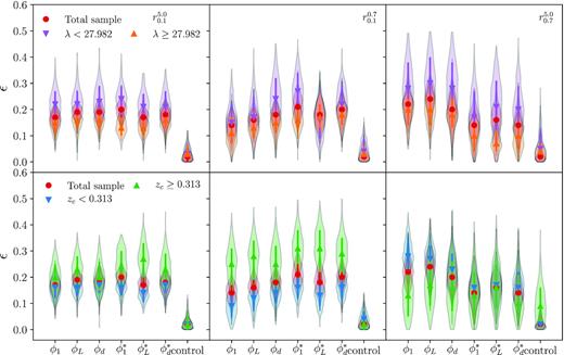
Posterior distributions of the average aligned ellipticity components, according to the different orientation angle criteria, for the total sample and low- and high-richness sample (upper panel) and for the total sample and low- and high-redshift samples (lower panel). Symbols and bars correspond to the median and error bars to the 16th and 84th percentiles of the posterior distributions. Left-hand, middle, and right-hand panels show the derived estimates fitting the quadrupole profiles within |$0.1\, h^{-1}_{70}$| Mpc|$\lt r \lt 5\, h^{-1}_{70}$| Mpc, |$0.1\, h^{-1}_{70}$| Mpc|$\lt r \lt 0.7\, h^{-1}_{70}$| Mpc, and |$0.7\, h^{-1}_{70}$| Mpc|$\lt r \lt 5\, h^{-1}_{70}$| Mpc, respectively.
In Fig. 6, we compare the ellipticities obtained by fitting the quadrupole profiles in the inner and outer regions, and with and without considering the membership cut in the satellite sample to estimate the orientation angle. The general tendencies discussed for the high- and low-richness and redshift samples can be also noticed in this figure. We do not observe a general tendency between the projected ellipticity estimates when the different weights (a uniform, a luminosity, and a distance weight) are considered to derive the orientation angle of the mass distribution. Taking into account the large dispersion observed in the distribution of differences of the derived angles (∼50 deg), the observed lack of impact of the weights on the ellipticity estimates, points to a general poorly orientation estimate of the mass distribution. Nevertheless, it can be noticed that the membership cut applied to the satellite samples used to compute the halo orientation, can affect differently the projected ellipticities in the inner and the outer regions of the quadrupole profile. To obtain information on how the membership cut in the computation of the surface density orientation affects the projected ellipticity estimates, we compute the ratio ϵ/ϵ*, defined as the ratio between the projected ellipticity estimated considering the whole sample of satellites to derive the orientation angle, ϵ, and using only the satellites that satisfy pmem > 0.5, ϵ*. For all the cluster samples, the proxy selection to define the halo orientation angle has a low impact on the derived projected ellipticities when the profiles are fitted over the whole projected radius range (|$r_{0.1}^{5.0}$|), being the average 〈ϵ/ϵ*〉 = 1.01 with a standard deviation of 0.12. Nevertheless, when the profiles are fitted up to |$700\, h^{-1}_{70}$| kpc (|$r_{0.1}^{0.7}$|), projected ellipticities tend to be higher if only the satellites with pmem > 0.5 are considered to estimate the orientation angle (〈ϵ/ϵ*〉 = 0.82 with a standard deviation of 0.15). This general tendency is reversed when the profile is fitted in the outer region (〈ϵ/ϵ*〉 = 1.60 with a standard deviation of 0.41). Therefore, the inner part of the halo is better traced by the satellites that have a higher probability of being members. On the other hand, the outer part of the projected density distribution is better traced by the whole sample of satellites.
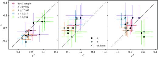
Derived average aligned ellipticity component estimates by fitting quadrupole profiles in the inner region (|$r_{0.1}^{0.7}$|, left-hand panel) and in the outer region (|$r_{0.7}^{5.0}$|, middle panel). The right-hand panel shows the ellipticities computed by fitting the quadrupoles in |$r_{0.1}^{0.7}$| (x-axis) and |$r_{0.7}^{5.0}$| (y-axis) ranges. ϵ* and ϵ refer to the ellipticity computed aligning the clusters according the satellites that satisfy the membership cut and the whole sample of satellites, respectively. Black and grey dots and crosses correspond to the quadrupoles computed considering the orientation angle weighting the satellites taking into account a distance, a luminosity, and a uniform weight, as defined in Section 3. Dashed grey line corresponds to the identity.
6 SOURCES OF BIAS IN THE ELLIPTICITY ESTIMATES
In this section, we discuss the possible effects that could bias our average aligned ellipticity component estimates and their impact in order to interpret our results. We are going to discuss the impact on the derived ellipticities of the misalignment between the major axis of the total mass distribution and the orientation angle estimated based on the satellite distribution. We also discuss how the selection effects of optical selected clusters can affect our ellipticity estimates. We do not intend to correct our measurements for the mentioned biases, but it is important to take them into account in order to interpret our results. All the discussed effects will bias our measurements to lower values, thus, we expect that the true projected ellipticity of the total mass distribution to be higher than the ϵ estimates. A detailed joint analysis using simulated data will be of a major importance to properly quantify these biases and will allow to link the estimates based on weak-lensing studies and the predicted projected ellipticities of dark matter haloes.
6.1 Misalignment effect
One of the largest source of bias is the fact that in principle, we do not know the actual major semi-axis orientation of the total mass distribution, since this is not necessary aligned with the satellite distribution. Moreover, even assuming that the satellites perfectly trace the dark mass distribution, there are many biases introduced when estimating the orientation angle according to the position of the galaxies classified as members. The main bias known as the Poisson sampling effect, is introduced due to the finite number of galaxies used to estimate the angle and it is specially important when a low number of satellites are considered or when the halo is more spherical (van Uitert et al. 2017). Mentioned misalignment will result in an underestimated ellipticity measurement, which will be related to the true projected mass ellipticity through equation (5).
If it is assumed that the galaxy distribution properly trace the dark matter, the ellipticities can be corrected by the Poisson sampling effect using simulations to evaluate the misalignment introduced as a function of the number of satellites and to estimate the correction factor. Shin et al. (2018) concluded that for the redMaPPer clusters the estimated ellipticity has to be corrected by a factor of ∼1.33, which represents a misalignment of 18°. The other sources of uncertainty introduced when computing the orientation angle are an edge effect, since members are selected within a circular aperture, and an effect introduced by the inclusion of interlopers. In principle, if we assume that interlopers have a random angular distribution, both effects will not introduce a bias in the estimated angle. Nevertheless these will introduce larger uncertainties in the angle estimates biasing the ellipticity to lower values.
6.2 Halo selection projection effects
Although redMaPPer clusters are considered one of the most homogeneous and well-calibrated catalogue of optical clusters, many studies have reported projection effects that can affect the sample (e.g. Dietrich et al. 2014; Costanzi et al. 2019; Sunayama et al. 2020). Mainly these effects have been studied in order to calibrate the richness–mass relation and to characterize their impact on cluster cosmology analyses. One of the sources of biases due to projection effects is related to the triaxiality, since optical selected clusters tend to be elongated along the LOS. This effect is proven to cause overestimated lensing masses in about |$3{\!-\!}6 {{\ \rm per\ cent}}$| and is more important for low-richness clusters (Dietrich et al. 2014). In that case, the lensing projected ellipticity will be also biased to lower values.
Another source of bias introduced by projection effects is related to the presence of LOS haloes, which are expected to be specially significant in rich galaxy clusters due to the abundance of correlated structures around these systems (Costanzi et al. 2019). Also, Sunayama et al. (2020) find a selection bias of optical cluster finders for clusters embedded within filaments aligned with the LOS. This increases both the observed cluster richness and the recovered lensing mass. Although the impact of LOS haloes in lensing measurements have already been extensively discussed (Abbott et al. 2020), most studies have mainly focused on the bias introduced on the mass estimates and the mass–richness relation. We stress here the impact on measurements of cluster ellipticities since we expect that this effect may be important and induce ϵ determinations to systematically lower values. First, the inclusion of interlopers in the satellite sample affects the mass distribution orientation estimate. Besides, LOS haloes with different projected orientations and at different projected distances from the cluster centre, will decrease the observed projected ellipticity. Finally, these projection effects can boost the halo mass, M200, which will affect the quadrupole fit.
7 DISCUSSION
In this section, we discuss the results obtained considering the potential biases presented in the last section. We first discuss the projected ellipticity of the dark matter haloes taking into account the average aligned ellipticity components obtained by fitting the quadrupole profiles in the inner regions. Then, we discuss how the derived projected ellipticities at the cluster outskirts might trace the accretion direction of the clusters.
7.1 Halo projected ellipticity
In order to get an insight regarding the projected shape of the haloes, we consider as the most representative parameter of the halo projected ellipticity, our estimates derived from fitting the quadrupole profile components up to |$700h^{-1}_{70}$| kpc, are obtained by aligning the clusters according to the |$\phi ^*_1$| proxy. This selection was made considering that the surface density at the inner regions is better traced by the galaxies with a higher membership probability (see Section 5) and since the derived ellipticities using a uniform weight are systematically larger for most of the considered samples. Nevertheless, we recall that no significant differences are observed for the different adopted weights. Taking this into account we obtain ϵ = 0.21 ± 0.04. Projected mean halo ellipticity of redMaPPer clusters were previously estimated by Clampitt & Jain (2016) and Shin et al. (2018). Clampitt & Jain (2016) derive the projected ellipticity of the redMaPPer clusters in a redshift range of 0.1 < z < 0.3, by aligning the systems according to the major semi-axis of the central galaxy. The authors report a halo ellipticity of 0.2, in agreement with our result for the low-redshift sample of clusters. van Uitert et al. (2017) also study the halo shape of less massive groups (1.5 × 10¹³ M⊙) using KiDS-450 shear catalogue, obtaining a projected ellipticity of 0.38 ± 0.12 by aligning the systems according to the BCG major semi-axis and fitting the profile up to 250 kpc. They also obtained ϵ = 0.49 ± 0.13 when considering the satellite distribution and fitting the quadrupole profile in a projected distance range from 250 up to 700 kpc, significantly higher than our ellipticity estimate. They discard the possible effect of neighbouring structures or a spurious lens–source alignment that could be biasing the result to higher values. On the other hand, Shin et al. (2018) estimated a mean projected halo ellipticity of 0.28 ± 0.07 considering a weak-lensing analysis of redMaPPer clusters within a similar redshift and richness range as those adopted in this work (0.1 < z < 0.41, 20 < λ < 200) but using shear catalogues based on SDSS observations, as in the previous Clampitt & Jain (2016) analysis. If we consider the correction factor for the Poisson sampling effect estimated by these authors, our corrected ellipticity measurement, 0.28 ± 0.05, is in excellent agreement with their estimate. This result is in agreement with the expectation from ΛCDM numerical simulations (Despali et al. 2017). However, it is important to take into account that we only consider for the comparison the introduced bias by the Poisson sampling effect. As discussed in the previous section, the other sources of misalignment and the selection effect of photometric clusters, will result in an underestimated projected ellipticity.
We obtain larger ϵ values for the samples selected at high-redshift (z ≥ 0.313) and low-mass clusters. For the low-mass clusters we estimate an average aligned ellipticity component of 0.27 ± 0.07 while for the high-mass clusters we obtain 0.16 ± 0.04. On the other hand, we obtain 0.16 ± 0.04 and |$0.31^{+0.07}_{-0.06}$| for the low- and high-redshift samples. In order to evaluate the error introduced by the sample dispersion, we performed a randomization test by fitting the parameters from 100 monopole and quadrupole profiles, derived by randomly selecting half of the total sample of clusters. The derived ϵ distribution has a mean of 0.21 and a standard deviation of 0.04, in excellent agreement with the values obtained for the total sample. Taking into account the previous analysis, we conclude that observed differences are not produced by sampling effects.
According to ΛCDM numerical simulations, it is expected that galaxy clusters at higher redshifts to be less spherical, since they are more affected by the direction of their major last merger, which is in agreement with our results. Also, the observed tendency between the low- and high-redshift cluster samples is obtained regardless which weight is considered in order to compute the cluster orientation angle. Furthermore, the average projected ellipticity estimated for the high-redshift sample (〈z〉 = 0.35), is in agreement with the analysis of Okabe et al. (2020) (see fig. 9 of their paper) based on the cosmological hydrodynamical simulation Horizon-AGN (Dubois et al. 2014).
Although with a low significance, the result obtained for the low- and high-mass samples is in disagreement with the expectation from isolated haloes in ΛCDM numerical simulations. Given that more massive haloes are formed later, they are expected to be less spherical. To test our result, we consider a higher redshift gap for the background galaxy selection, taking Z_BEST > zc + 0.3, and we recompute the profiles. This test is motivated by the fact that a larger fraction of red galaxies is expected at the location of higher mass clusters. These cluster member objects can contaminate the sample of background galaxies inducing a dilution of the lensing signal. Derived ellipticities from the profiles obtained with this new background galaxy sample are 0.11 ± 0.06 and 0.31 ± 0.08 for the high- and low-mass cluster samples, respectively. This suggests that the observed gap is not due to a bias introduced by the selection of background galaxies.
It is important to highlight that the projected ellipticities estimates for the low- and high-mass samples, are in agreement within 1σ. Moreover, if we consider a different weight to estimate the orientation angle of the mass distribution than the adopted uniform weight, i.e. if the aligned ellipticity component is obtained according to |$\phi ^*_d$| or |$\phi ^*_L$|, the difference between the fitted values is even lower. However, we cannot neglect the possibility that the effects introduced by the contribution of the surrounding haloes on the LOS can bias the projected ellipticity estimate to lower values, affecting mainly the higher richness sample. The use of numerical simulations to measure the projected ellipticity, mimicking the same approach of this analysis (i.e. defining an axis from the galaxy distributions and measuring the lensing signal accounting for the matter along the LOS) can be of great importance to study the biases discussed and to assess quantitatively their impact on the lensing estimates.
7.2 Projected density distribution at the cluster outskirts
Here, we intend to discuss how the projected density mass is distributed at the outskirts of the clusters by considering the fitted projected ellipticities at the outer regions of the quadrupole profiles (|$r \gt 700h^{-1}_{70}$| kpc). In order to do that, we consider the projected ellipticities derived by aligning the clusters taking into account ϕ1, since, as discussed in Section 5, the whole sample of members traces better the mass distribution at larger distances from the cluster centre (see Figs 5 and 6). The membership cut can be useful to discard interlopers, since their inclusion could result in a wrongly estimate of the orientation angle, thus underestimating the projected ellipticity. However, this sample of satellites could be also including galaxies that have been recently accreted by the cluster. pmem is computed according to the galaxy colour, luminosity, and projected distance from the cluster centre. Therefore, satellites with pmem < 0.5 are in principle dimmer, bluer and located at larger distances from the cluster centre. The observed result might suggest that the outer region is better traced when pmem < 0.5 satellites are included, since this sample include bluer galaxies that were accreted later and thus follow the mass distribution at the cluster outskirts.
Similarly to the inner region, which is more related to the halo projected elongation, low-mass systems tend to show larger aligned ellipticity component values in the outer regions, being |$0.28_{-0.09}^{+0.10}$|, while for the high-mass sample we obtain |$0.20_{-0.06}^{+0.04}$|. Nevertheless, both results are in agreement taking into account the errors. On the other hand, derived ellipticities at the outskirts for the low-redshift sample is larger than for high-redshift clusters, being |$0.28_{-0.05}^{+0.06}$| and 0.13 ± 0.08, respectively. This tendency also can be observed in the right-hand panel of Fig. 6, in which the inner and outer ellipticities are uncorrelated for the two redshift samples, being the outer regions less spherical for the low-redshift sample, while the high-redshift sample is less spherical when the profile is fitted up to 700 kpc. This result can be interpreted as the projected density distribution may be better traced by the inclusion of bluer galaxies at lower redshifts.
8 SUMMARY AND CONCLUSIONS
In this work, we presented a study of the surface mass density shape of galaxy clusters, through the estimated aligned component of the projected ellipticity using weak-lensing techniques. We used the optically selected SDSS redMaPPer clusters within a redshift and a richness range of 0.1 ≤ z < 0.4 and 20 ≤ λ < 150, respectively. The weak-lensing analysis was performed taking advantage of the combination of four high-quality shear catalogues. We modelled the derived lensing signal taking into account a multipole expansion of the surface density distribution. The total surface density was modelled considering two terms that include the monopole and a quadrupole, where the quadrupole is proportional to the projected ellipticity. Quadrupole profiles were computed by aligning the clusters taking into account the satellite distribution, for which we consider six different proxies. Finally, we fit the profiles in three projected radius ranges to obtain information regarding the shape of the mass distribution at the inner and outer regions of the clusters.
Derived ellipticities by fitting the profile up to |$700h^{-1}_{70}$| kpc are larger if a membership cut is applied to the satellites considered to estimate the orientation angle. Therefore, the inner regions are better traced by the galaxies that have a higher membership probability. On the other hand, projected ellipticity values are larger if the profiles are fitted in the outer regions (|$\gt 700h^{-1}_{70}$| kpc) when all the galaxies classified as members are included to estimate the orientation of the mass distribution. Therefore, the inclusion of bluer galaxies mainly located at larger projected radius, trace better the density distribution at the outskirt of the clusters.
To study the mean halo projected ellipticity we consider the estimates derived by fitting the profile at the inner regions. For the total sample of clusters we derive a projected ellipticity of 0.21 ± 0.04. If we consider the Poisson sampling effect, which takes into account that the orientation angle is estimated from a finite number of galaxies, we obtain 0.28 ± 0.04, in excellent agreement with previous estimates (Shin et al. 2018). Although this result is also in agreement with the predicted by numerical simulations (Despali et al. 2017), a detailed quantification of possible biases is important in order to link the weak-lensing projected ellipticity estimates with the dark matter halo expected elongation.
We also analyse the dependence of the derived cluster projected ellipticity estimates on the mean mass and redshift of these systems. This is accomplished by splitting the sample into two bins considering the median values of richness and redshift of the total sample, respectively. We obtain a larger mean projected ellipticity for the high-redshift cluster, in agreement with the expectation of ΛCDM numerical simulations. Also, we obtain a tendency for a smaller projected ellipticity in the high-mass cluster sample, although its significance is low. Moreover, it should be considered that a higher contribution of the surrounding clusters distributed mostly along the LOS, could be biasing the projected ellipticity of the richest clusters to lower values. A further analysis on the projection effects of optically selected clusters and their influence on the lensing ellipticity measurements is required to characterize properly the mean projected halo elongation.
Finally, we study the density mass distribution at the outskirts, considering the ellipticity estimates obtained by fitting the profile at the outer regions and the whole sample of galaxy members to align the clusters. No significant differences are observed for the low- and high-mass cluster samples. Nevertheless, we derive a larger mean ellipticity for the low-redshift cluster sample than for the high-redshift sample. This result can be indicating a more constrained direction of the matter accretion region at lower redshifts.
Taking advantage of the combination of high-quality weak-lensing data, we presented the analysis of the projected shape of the cluster-sized haloes and its relation with the mass and redshift. We study the mass distribution at the cluster outskirts, which can be related to the large-scale structure and can provide information about the matter accretion of these galaxy systems. This work anticipates the full potential of the weak gravitational lensing techniques in the study of the average projected mass distribution shape of galaxy clusters. Recently release of DES-Y1 based on the Dark Energy Survey (DES; The Dark Energy Survey Collaboration 2005), provides a new sample of redMaPPer clusters spanning a larger redshift and richness range that will allow a deeper study of halo shape and the general projected mass distribution of galaxy clusters. Moreover, new upcoming data based on DES and on the forthcoming ‘The Rubin Observatory Legacy Survey of Space and Time’ (LSST; The LSST Dark Energy Science Collaboration 2018) and on the EUCLID mission (Amendola et al. 2013), will offer a larger statistical sample of galaxy clusters plus high-quality shear catalogues that will allow a deeper study on the relation of the projected halo elongation with the redshift and mass. These studies combined with the predictions from simulations, can shed light regarding the shape evolution of dark matter haloes and their accretion history.
ACKNOWLEDGEMENTS
This work was partially supported by the Consejo Nacional de Investigaciones Científicas y Técnicas (CONICET, Argentina), the Secretaría de Ciencia y Tecnología de la Universidad Nacional de Córdoba (SECyT, UNC, Argentina), the Brazilian Council for Scientific and Technological Development (CNPq), and the Rio de Janeiro Research Foundation (FAPERJ). We acknowledge the PCI BEV fellowship program from MCTI and CBPF. MM acknowledges FAPERJ and CNPq for financial support. FORA BOZO. HYS acknowledges the support from NSFC of China under grant 11973070, the Shanghai Committee of Science and Technology grant no. 19ZR1466600 and Key Research Program of Frontier Sciences, CAS, grant no. ZDBS-LY-7013. LVW acknowledges the support from the Natural Sciences and Engineering Research Council of Canada. This work is based on observations obtained with MegaPrime/MegaCam, a joint project of CFHT and CEA/DAPNIA, at the Canada–France–Hawaii Telescope (CFHT), which is operated by the National Research Council (NRC) of Canada, the Institut National des Sciences de l’Univers of the Centre National de la Recherche Scientifique (CNRS) of France, and the University of Hawaii. The Brazilian partnership on CFHT is managed by the Laboratório Nacional de Astrof ísica (LNA). We thank the support of the Laboratório Interinstitucional de e-Astronomia (LIneA). We thank the CFHTLenS team for their pipeline development and verification upon which much of the CS82 survey pipeline was built.
This research used the facilities of the Canadian Astronomy Data Centre operated by the National Research Council of Canada with the support of the Canadian Space Agency. RCSLenS data processing was made possible thanks to significant computing support from the NSERC Research Tools and Instruments grant program. Based on data products from observations made with ESO Telescopes at the La Silla Paranal Observatory under programme IDs 177.A-3016, 177.A-3017, and 177.A-3018.
DATA AVAILABILITY STATEMENT
The data sets were derived from sources in the public domain: CFHTLenS (http://www.cadc-ccda.hia-iha.nrc-cnrc.gc.ca/en/community/CFHTLens), RCSLenS (https://www.cadc-ccda.hia-iha.nrc-cnrc.gc.ca/en/community/rcslens), KiDS-450 (http://kids.strw.leidenuniv.nl/cosmicshear2018.php), and redMaPPer (http://risa.stanford.edu/redmapper/). CS82 can be accessed on request by emailing to martincbpf.br. The data derived in this article are available on request to the corresponding author.
Footnotes
Throughout this work we consider satellite galaxies as the galaxies that were classified as cluster members, besides the central galaxy. These galaxies are supposed to be located at the satellite haloes, hosted in the main dark matter halo of the cluster.
REFERENCES
APPENDIX A: TESTING THE COMBINATION OF THE WEAK-LENSING CATALOGUES
In order to test the combination of the weak-lensing shear catalogues presented in Section 2, we compute the monopole and quadrupole profile components considering the individual shear catalogues. For this purpose, we consider the total sample of clusters used in this work. Derived monopole and quadrupole profiles scaled according to the projected distance to emphasize the differences are shown in Figs A1 and A2, respectively. As it can be noticed, not significant biases are observed in the computed profiles. We also fitted the monopoles computed using the shear catalogues separately and the quadrupoles computed considering the orientation angle estimated using the whole sample of galaxy members and a uniform weight. Results are presented in Table A1. All the parameters are in agreement within 1σ with the resulting fitting values derived using the combined catalogues. We also show the contribution of the different catalogues to the total sample of background galaxies, where the CFHTLens catalogue provides the largest fraction of source galaxies.
![Tangential (upper panel) and cross (bottom panel) components of the shear monopole scaled according to the projected distance in units of [Mpc M⊙ pc−2], computed considering the used shear catalogues individually.](https://oup.silverchair-cdn.com/oup/backfile/Content_public/Journal/mnras/501/4/10.1093_mnras_staa3570/1/m_staa3570figa1.jpeg?Expires=1750734539&Signature=vlKbfdOvxT1taYtBUPs2N8acKwIB-WWPHLhET8LP~6Xq2nXd8kTc2JHWmxLwK5IB-G~lGFCEkAAtXBMeZosdo6y~iRKoRJtVukxqGOO6b8vYK0-o2mjIe-TnhwLFGAx1fuuspR3wf7cXq3iznLgq3R-7Y8dKKS9TaMBeQY8Hd3rdnzO00~OTlr4VZ-GQWOImJMQFgCq9gv61GTH~S-wXIZ2pmZADXy39e80BJ1mc3WbMjOj2ukEXlZV8TUxTF-olLC0soMmViK58A2wPUMJ3RI0absoFCYA8UNg~Dt9zGGeexMqNp8yxuD1VE7wQC~QtSIgf5xAeAEp6JvrDBB8fnQ__&Key-Pair-Id=APKAIE5G5CRDK6RD3PGA)
Tangential (upper panel) and cross (bottom panel) components of the shear monopole scaled according to the projected distance in units of [Mpc M⊙ pc−2], computed considering the used shear catalogues individually.
![Tangential ($\Gamma _{\rm {t} \cos {2\theta }}$) and cross ($\Gamma _{\rm {\times } \sin {2\theta }}$) components of the quadrupoles scaled according to the projected distance in units of [Mpc M⊙ pc−2], computed considering the used shear catalogues individually for the different orientation angle proxies.](https://oup.silverchair-cdn.com/oup/backfile/Content_public/Journal/mnras/501/4/10.1093_mnras_staa3570/1/m_staa3570figa2.jpeg?Expires=1750734539&Signature=0T7PeQJ5lW6M13mN-VoNZWxLmdnEuqaB24x4FVtu~vobcjWQsv05sA9I5TjMIGeQwLOuy0oty8PNwBXlF1LE44E9juBkQI33IjmKsjkR0ZQ7jtWpyj0fttm32kpmPIcYUIyRhsCTWVNzQGjCt-cIdVGpkRw-gavYFm5JFScEUR3KqXoOtfUCHsEuru-0GEXUP0cxDlHfzsM8KhY1K3j5pz1a96mNSQJS31h0ZWSyHO-NSbXQRNZX60SC66N8oipcietKhuHv3TkwSeOlPYUFErMQydxiTEeuBINfNFYgb-dASgyt0pJ0hocU-dMJbsaw33ZP9RsLW1umnkZH4kgMNQ__&Key-Pair-Id=APKAIE5G5CRDK6RD3PGA)
Tangential (|$\Gamma _{\rm {t} \cos {2\theta }}$|) and cross (|$\Gamma _{\rm {\times } \sin {2\theta }}$|) components of the quadrupoles scaled according to the projected distance in units of [Mpc M⊙ pc−2], computed considering the used shear catalogues individually for the different orientation angle proxies.
Fitted parameters from the monopole and quadrupole profile components computed using the combined weak-lensing shear catalogues and each individual catalogue.
| Shear catalogue | NL | NS/NT | M200 | pcc | ϵ |
|---|---|---|---|---|---|
| Combined | 2275 | 1 | |$2.06_{-0.11}^{+0.09}$| | |$0.79_{-0.04}^{+0.04}$| | |$0.17_{-0.03}^{+0.03}$| |
| CFHTLens | 311 | 0.30 | |$2.09_{-0.15}^{+0.18}$| | |$0.85_{-0.08}^{+0.07}$| | |$0.18_{-0.05}^{+0.06}$| |
| CS82 | 662 | 0.24 | |$1.84_{-0.13}^{+0.15}$| | |$0.82_{-0.07}^{+0.06}$| | |$0.25_{-0.05}^{+0.05}$| |
| KiDS-450 | 684 | 0.28 | |$2.06_{-0.20}^{+0.16}$| | |$0.74_{-0.07}^{+0.07}$| | |$0.09_{-0.05}^{+0.06}$| |
| RCSLens | 1005 | 0.19 | |$1.93_{-0.18}^{+0.18}$| | |$0.81_{-0.07}^{+0.07}$| | |$0.15_{-0.06}^{+0.05}$| |
Note. Columns: (1) weak-lensing shear catalogues; (2) number of clusters considered for the stacking, (3) fraction of background galaxies included in each catalogue; (4) mass in units of [|$h^{-1}_{70} 10^{14}\, \mathrm{ M}_\odot$|]; (5) fraction of well-centred clusters derived from the monopole fit; and (6) constrained projected ellipticity.
APPENDIX B: QUADRUPOLE PROFILES
In this appendix, we present the quadrupole profiles together with their best-fitting models. We show in Fig. B1 the quadrupoles derived for the total sample of the redMaPPer clusters. In Figs B2 and B3, we show the profiles computed for the high- and low-mass cluster samples and for the high- and low-redshift samples, respectively. Derived best-fitting ellipticities are detailed in Table 2.
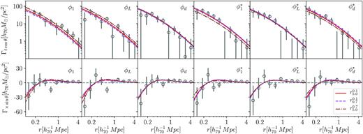
Derived quadrupole tangential and cross component profiles, Γtcos θ and Γ× sin θ, for the total sample of redMaPPer clusters analysed in this work. Best fits for the three different considered radius ranges are also shown. Quadrupoles are obtained taking into account the derived orientation angles computed for each cluster according to the proxies defined in Section 3 (|$\phi _1,\phi _L,\phi _d,\phi ^*_1,\phi ^*_L$|, and |$\phi ^*_d$|).
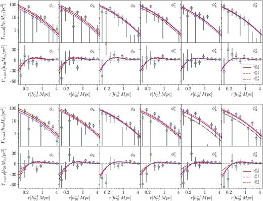
Idem as in Fig. B1 but for the low-mass (upper panel) and high-mass (bottom panel) cluster samples, selected according to the median of the richness distribution.
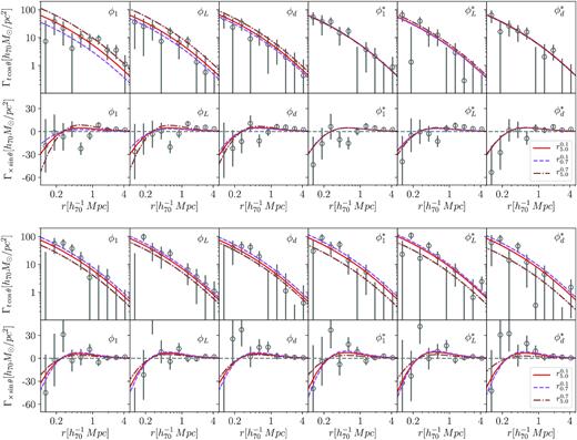
Idem as in Fig. B1 but for the low-redshift (upper panel) and high-redshift (bottom panel) cluster samples, selected according to the median of the redshift distribution.
