


ABSTRACT
The completeness of the Gaia catalogues heavily depends on the status of that space telescope through time. Stars are only published with each of the astrometric, photometric, and spectroscopic data products if they are detected a minimum number of times. If there is a gap in scientific operations, a drop in the detection efficiency or Gaia deviates from the commanded scanning law, then stars will miss out on potential detections and thus be less likely to make it into the Gaia catalogues. We lay the groundwork to retrospectively ascertain the status of Gaia throughout the mission from the tens of individual measurements of the billions of stars, by developing novel methodologies to infer both the orientation and angular velocity of Gaia through time and gaps and efficiency drops in the detections. We have applied these methodologies to the Gaia data release 2 variable star epoch photometry – which are the only publicly available Gaia time-series at the present time – and make the results publicly available. We accompany these results with a new python package scanninglaw that you can use to easily predict Gaia observation times and detection probabilities for arbitrary locations on the sky.
1 INTRODUCTION
Gaia (Gaia Collaboration 2016) is the first all-sky astrometric, photometric, and spectroscopic survey with tens to hundreds of repeat observations over a decade-long baseline. Future Gaia data releases (DR) will drive a generational breakthrough in our ability to carry out time-domain astrophysics, allowing us to study binary stars, exoplanets, variable stars, supernovae, and microlensing events through combinations of epoch astrometric, photometric, and spectroscopic measurements. Our ability to discover a transient source or detect the variability of a periodic source will depend on both the number of Gaia observations and the timings between them (as well as the uncertainties of the individual observations). The pattern of these Gaia observations varies systematically across the sky – as described by the scanning law which states where Gaia was looking at every point in time – and thus we will be differently able to investigate time-domain phenomena in different regions of the sky. The picture is further complicated by the possibility that a Gaia observation predicted by the scanning law may not result in a published measurement, as that can change the completeness and sensitivity of the Gaia pipeline to time variable objects at that location on the sky. The set of variable and non-variable objects in the Gaia catalogues will be biased by the selection function resulting from the effective scanning law that was used, and we will not be able to make unbiased general statements unless we can correct for these biases, which will require us (amongst other things) to know when Gaia looked at a given point on the sky and the probability that each of those observations would have resulted in a measurement of a given star. It is thus of fundamental importance that we have a precise knowledge of the Gaia scanning law, the reasons why a Gaia observation might not result in a published measurement, and the times when no Gaia measurements were acquired.
In Boubert, Everall & Holl (2020, hereafter referred to as Paper I), we conducted preliminary work towards that goal by exploiting the light curves of the 550 737 variable sources published in Gaia DR2 (Evans et al. 2018; Gaia Collaboration 2018; Holl et al. 2018; Riello et al. 2018), which tell us the time of each detection and the location of the detection on the Gaia focal plane. By aligning the reported location of the source on the focal plane with the location of the source on the sky, we were able to derive first-order corrections to the Gaia DR2 nominal scanning law1 (the scanning law that DPAC (Data Processing and Analysis Consortium) commanded Gaia to follow and which can deviate from the true scanning law by up to 30 arcseconds). By looking at the times between consecutive photometric measurements of all of the variable stars, and by comparing the predicted number of observations at each location on the sky to the reported maximum number of astrometric, photometric, and spectroscopic detections, we were able to identify ‘gaps’ which contributed no detections to the published catalogue.
Boubert & Everall (2020, hereafter referred to as Paper II) relied on the results of Paper I to accurately predict the number of observations of each source that could have resulted in detections (i.e. those not during a period which did not result in any published detections). Paper II used this information to model the probability that the Gaia DR2 observations of a source at any location on the sky resulted in at least five detections – the minimum requirement for a source to enter the Gaia DR2 source catalogue – and thus arrived at an approximation to the Gaia DR2 selection function. However, there were several deficiencies in Paper I which we will address here. First, our corrections to the scanning law were simplistic and only corrected the pitch and roll of Gaia, not the yaw. Our corrected scanning law was thus able to predict the across-scan location of the source to a precision of 0.083 arcsec, but the along-scan location remained uncertain at a level of 30 arcsec, with a corresponding uncertainty on the timing of predicted observations of 0.5 s. Second, we defined a gap to have occurred between any two consecutive photometric measurements more than 1 per cent of a day apart without a robust statistical justification. This may have caused us to both miss shorter gaps and to erroneously interpret long intervals between consecutive observations as gaps in regions of the sky that are simply sparse in variable stars. Third, we ignored that another reason for a Gaia observation not to have resulted in a published detection is if that detection is deleted on-board due to Gaia scanning dense regions of the sky for large fractions of the spin period and exhausting its available storage capacity due to the limited down-link bandwidth. This will result in a magnitude-dependent deletion fraction that varies as a function of time as Gaia scans across more and less dense parts of the sky. Fourth, we ignored that there are other processes besides gaps and on-board deletions that can cause an observation to not result in a published detection, ranging from faint sources not being detected every time due to photon shot noise to crowding preventing every source from being assigned a window to quality cuts applied by the Gaia DPAC as listed in the Introduction of Paper I.
It is likely that we will not be able to identify with full certainty the nature of all of the processes that caused observations to be missed. Instead, our goal in this work is to characterize the time-varying and partially probabilistic process through which Gaia observations result in published detections, to the best degree possible with the 550 737 light curves associated with Gaia DR2 variable sources. Our methods will be immediately applicable to larger samples of Gaia epoch measurements when they are made available in later DR. The fourth and subsequent Gaia DR will contain all of the epoch astrometric, photometric, and spectroscopic measurements and an extension of this methodology will allow the community to diagnose the photometric and temporal biases impairing the completeness of these DR.
This work consists of two parts. In Section 3, we use the locations of the variable stars both on the focal plane and on the sky at their times of detection to infer Gaia’s orientation and angular velocity throughout the 22 months of Gaia DR2. In Section 4, we combine the detection times of the variable stars with the predicted observations that did not result in published detections to simultaneously infer gaps which did not result in any published detections and the magnitude dependency of the detection probability with time. The methodologies in both sections are based on temporally evolving state space models and so we begin with a pedagogical overview of Gaussian process regression, Hidden Markov Models, and Kalman filters in Section 2.
2 MODELLING STATES THROUGH TIME
Throughout this paper, we will consider probabilistic models with time-evolving state parameters |$\boldsymbol{\theta }(t)$| that describe some aspect of a process that we are interested in. At discrete times |$\lbrace t_{i}\rbrace _{i = 1}^{n}$|, we make a noisy measurement of either those parameters, a function of those parameters, or random variables that are conditioned on those parameters. The latter two cases are known as hidden state spaces, because we never have direct access to the values of the state parameters. In this section, we give an overview of such models as a precursor to the other sections in this work.
2.1 Gaussian process regression
The first term of this expression is the covariance kernel for the underlying time-series, and the second is the covariance kernel for the noise in each observation, with σ(ti) being the known noise of the measurement at time ti. We call the hyperparameter μ the ‘signal mean’, ε2 the ‘signal variance’ and l the ‘time-scale’, and collate them in the hyperparameter vector |$\boldsymbol{\xi }=[\mu ,\varepsilon ^2,l]$|.
We will use Gaussian process regression in Section 4.1 to fill in missing values in the Gaia DR2 variable star light curves, by inferring the magnitudes of the stars at the predicted observation times that did not yield published detections.
2.2 Hidden Markov Models
Hidden Markov Models are used to model a system that is known to transition between discrete states through a Markov Process X, but where we do not have direct access to the value of the states |$\lbrace X_i\rbrace _{i=1}^n$|. There is assumed to be another discrete process Y whose states |$\lbrace Y_i\rbrace _{i=1}^n$| are conditioned on process X and are observed, and so the task is to infer the states of process X given the observed states of process Y. For instance, the lead author regularly travels by train from Oxford to London. Whether that train leaves Oxford on time on a particular day (Yi = 1) or not (Yi = 0) is conditionally dependent on whether there were leaves on the track between Hereford and Oxford (Xi = 1) or not (Xi = 0). The lead author will not know if there were leaves on the track, but the train is more likely to be running late if this was the case. The probability of there being leaves on the track will depend in some way on whether there were leaves on the track the previous day, for instance through the weather or the number of leaves left on the trees.
We will use a Hidden Markov Model in Section 4.2 to identify gaps when Gaia observations were not resulting in published detections.
2.3 Kalman filters
3 SCANNING LAW
Determining the Gaia scanning law is exactly analogous to the problem of determining the attitude of Gaia through time. Determining the attitude of a spacecraft is a key engineering challenge which has been covered extensively in the literature (see Wertz 2012, and references therein), although our use case is peculiar in that we do not have access to gyroscopic2 measurements or data from a star tracker. Instead, we will attempting to infer the attitude of Gaia based on the nominal scanning law and the locations and timings of the detections of the Gaia DR2 variable stars. Note that in the post-processed Astrometric Global Iterative Solution of Gaia (AGIS, see Lindegren et al. 2012) the attitude is also derived from the observations themselves, though based on a set of ‘primary’ sources that behave like single point-like sources whose colour is stable. Gaia’s point spread function is colour-dependent (Lindegren et al. 2018) and so if a source’s colour changes with time then that adds additional uncertainty into the determination of its position. Variable stars have colour variations and could be components of astrometric binary systems, both of which make them less than ideal as reference sources for the extreme attitude precision that the official astrometric solution requires, but are the only sources for which we have Gaia time-series. We chose to use the first-order multiplicative extended Kalman filter (MEKF, Markley 2003) where the attitude of the spacecraft is expressed as a quaternion, the attitude error is multiplicative, and the attitude error and angular velocity vector are assumed to be hidden states that jointly satisfy a multivariate normal distribution at all times. We use quaternions as they are the ideal mathematical object to encode the orientation of a spacecraft (an argument developed in the following section) and were used in the AGIS (Lindegren et al. 2012) to determine Gaia’s attitude for the official Gaia DPAC astrometric solution.
3.1 What are quaternions?
3.2 Positions of stars on the sky and on the focal plane
We are attempting to infer the attitude of Gaia with very little information. Traditionally, the attitude of a spacecraft is inferred using measurements from a combination of gyroscopes and star trackers, but we do not have access to these. We have only access to the light-curves of the 550 737 stars classified as photometrically variable by DPAC in Gaia DR2. Each of the flux measurements in those light curves has an associated transit_id which encodes the time t, the field of view F, and the across-scan pixel P and CCD C of the detection on the Gaia focal plane. In the Gaia body frame, the along-scan angles are the longitude and the across-scan angles are the latitude, so named because they point in directions parallel and perpendicular to the direction in which Gaia is scanning. Note that technically the transit_id encodes the centre of the window that was assigned on-board to record the flux around the identified point source. Both time and position in the transit_id are from the on-board estimates, which have an uncertainty of roughly 1 pixel, that is, ∼60 mas in the along-scan direction (corresponding to ∼1 ms) and ∼180 mas in the across-scan direction. As we do not have access to the sub-pixel centroid estimate for each window, the precision of each transit observation will hence be limited to about 1 pixel in both directions. The timings of the detections are those measured on-board Gaia and so will be subject to aberration effects, while the timings of the brightest detections (G < 12) could be offset due to the partial, gated integrations used to prevent saturation.
It is more important to accurately know the across-scan location of a source than the along-scan location, because in the latter case a 20 arcsec offset will only cause an error of 0.3 s in the observation time, while in the former case it might mean that the star falls outside of Gaia’s field of view. Relativistic aberration is caused by Gaia’s motion around the Sun of roughly 30 km s−1 (Gaia is located at L2 and so moves at approximately Earth’s orbital velocity), which can result in a maximum total aberration of about 20 arcsec (see equation 17 of Klioner 2003) across a combination of the along- and across-scan directions. Due to the importance of the across-scan location being correct, we corrected for the effect of aberration as described later in this section. The gating can only cause the detection location to be off in the along-scan direction by at most half of a CCD integration time (the ungated CCD integration time is 4.42 s (see section 2.2 of Crowley et al. 2016)) and so the predicted observation times of the gated brightest stars can be off by at most 2.2 s. Errors of these scales in the predicted observation time will not be astrophysically important even for stars exploding as supernovae, justifying us to neglect this effect.
Given the geometry of the Gaia focal plane, there are functions η(F, P, C) and ζ(F, P, C) that map these quantities to along- and across-scan angles in the body frame of Gaia, which can then be expressed as a unit vector. The attitude of Gaia at the time of detection can then be used to rotate that unit vector to the ICRS reference frame. However, we already know the location of the star on the sky from the Gaia DR2 source catalogue and thus we can constrain the unknown attitude at the time of the detection by requiring that the location of the star on the focal plane aligns with the location of the star on the sky. We note that – even if the position of the star on the sky and the geometry of the focal plane is known perfectly – the alignment of one vector in the body frame with one in the reference frame only constrains two of the three degrees of freedom in the attitude.
Suppose that at this epoch we have an uncertain estimate of the attitude of Gaia |$\boldsymbol {\delta q}(\boldsymbol {a})\otimes \hat{{\boldsymbol q}}$| parametrized by |$\boldsymbol {a}$| with mean |$\hat{\boldsymbol {a}}=0$| and covariance |$\boldsymbol{\sf P}_{aa}$|, then – to first order in the uncertainties of the attitude and the unit vector in the reference frame – the predicted unit vector in the body frame of Gaia has mean |$\boldsymbol{\sf A}(\hat{{\bf q}})\vec{u}$| and covariance |$\boldsymbol{\sf H}_a\boldsymbol{\sf P}_{aa}\boldsymbol{\sf H}_a^T+\boldsymbol{\sf A}(\hat{{\boldsymbol q}})\boldsymbol{\sf S}\boldsymbol{\sf A}^T(\hat{{\boldsymbol q}})$|, where |$\boldsymbol{\sf H}_a = [\hat{\boldsymbol {u}}\times ]$|. The second term is simply the rotation of the uncertainty in the unit vector in the reference frame and we refer the reader to Markley (2003) for details on the first term.
The key to the MEKF that we will describe in the following section is the measurement update step: the uncertain unit vector in the Gaia body frame pointing from Gaia to a source is predicted using our current estimate of Gaia’s attitude, thus allowing us to use the unit vector deduced from the field of view, CCD, and pixel of the detection as a measurement to constrain the attitude.
3.3 The multiplicative extended Kalman filter
The MEKF is a modification of the extended Kalman filter described in Section 2.3 that allows for part of the state – the attitude of the spacecraft – to be constrained to have unit normalization. We stress that the overview of the MEKF presented here draws heavily from Markley (2003), who presented one of the seminal overviews of the MEKF, and Burton et al. (2017), who adapted the MEKF for the case where the attitude needed to be determined based on noisy measurements of the vector pointing towards the Sun rather than measurements from a gyroscope or star tracker.
Analogously with Section 2.3, we define |$\hat{{\boldsymbol q}}_{i|j}$|, |$\hat{\boldsymbol {\omega }}_{i|j}$|, and |$\boldsymbol{\sf P}_{i|j}$| to be our estimate of the mean attitude quaternion, mean angular velocity vector, and covariance between the attitude error and angular velocity vectors at time ti given all of the measurements made at times up to and including time tj. The MEKF iteratively calculates the quantities |$\hat{{\boldsymbol q}}_{i|i}$|, |$\hat{\boldsymbol {\omega }}_{i|i}$|, and |$\boldsymbol{\sf P}_{i|i}$| at each time-step given all of the prior observations. Each time-step is split into a prediction and a measurement update stage.
3.4 Application of the MEKF
Our model of the attitude of Gaia has four free parameters – the variance |$\sigma _{\mathrm{MEKF}}^2$| of the random angular accelerations experienced by Gaia, the excess spread in the locations of the star on the focal plane |$\sigma _p^2$| and the corrections to the CCD δc and pixel δc across-scan widths. If we propose a set of values for these parameters and provide a set of detections of Gaia sources then the MEKF algorithm described above will churn out a log-likelihood, and so we are able to carry out maximum-likelihood estimation of the values of those parameters. We opt to split the 22 months of Gaia DR2 into day-long chunks and perform maximum-likelihood optimization separately in each day. We do this to make our estimation more robust to extreme adverse events; if Gaia’s attitude rapidly changed in one short period then that could cause the value of |$\sigma _{\mathrm{MEKF}}^2$| to be biased high. The MEKF is a recursive algorithm and so cannot be naively parallelized, and so splitting the optimization into chunks also makes the optimization more computationally tractable by allowing it to be spread across multiple CPUs. We performed the optimization using the scipy implementation of the Nelder–Mead algorithm (Gao & Han 2012). The initial attitude and angular velocity vector was taken from the last time point of the nominal scanning law prior to the first data point in that day. We note that the nominal scanning law as provided by DPAC has a discontinuity on the 2014 September 25 (OBMT = 1326.7 rev), which corresponds to the transition from the original nominal scanning law to one optimized for the ‘GAia Relativistic Experiment on Quadrupole’ experiment (de Bruijne et al. 2010). This transition created a discontinuity in the phase of both the precession and spin. Whilst in reality Gaia would smoothly transition to the updated scanning law, the nominal scanning file has an abrupt transition with the attitude changing by more than 100° between two consecutive 10 s time-steps. This transition occurs during the data-taking gap associated with the first decontamination of Gaia and so is not constrained by the variable star detections. We reset the MEKF at that time point by resetting the attitude and angular velocity to that given by the nominal scanning law after the transition.
In Fig. 1, we show a corner plot of the maximum-likelihood values of (σMEKF, σp, δc, δp) from each of the 667 d. We estimate the values of our parameters from the (16, 50, 84) per cent percentiles of this forest of maximum-likelihood values to be |$\sigma _{\mathrm{MEKF}} = 1.28_{-0.08}^{+0.06}\,\,\mu \mathrm{as}\,\,\mathrm{s}^{-2}$|, |$\sigma _{p} = 56.04_{-3.10}^{+5.76}\,\,\mathrm{mas}$|, |$\delta _{c} = 31.61_{-3.33}^{+6.13}\,\,\mathrm{mas}$|, and |$\delta _{p} = -43.70_{-3.23}^{+1.80}\,\,\mathrm{mas}$|. The values of the latter three of these parameters (shown as blue lines in Fig. 1) are in excellent agreement with our findings in Paper I, giving us faith in the results of these two independent methodologies, though the value of σp is slightly smaller due to us mistakenly ignoring aberration in the previous work. We verified that if we neglected aberration in this work then we recovered the larger value of σp.
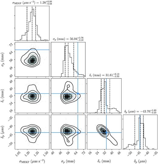
Corner plot of the hyperparameters of our Gaia attitude model, determining the random angular accelerations experienced by Gaia (σMEKF), the excess error in the location of the stars (σp), and the along-scan corrections to the CCD δc and pixel δp widths. The blue lines indicate the values that the latter three of these hyperparameters took in our much simpler model of Gaia’s attitude in Paper I.
Adopting the median values of the parameters as our fiducial values, we inserted the nominal scanning law time-points into the MEKF as time points without a measurement update step and calculated the means and covariances of the attitude and angular velocity at those time-steps, employing the MEKF with the additional backwards smoothing step. In Figs 2 and 3, we show the across- and along-scan distance between the locations of the two fields of view in our corrected scanning law and their locations in the nominal scanning law, in the frame of the nominal scanning law. The across-scan offsets of the two fields of view have medians (12.9 and −11.4 arcsec, respectively) that are significantly different from zero, indicating either a long-term difference between the two scanning laws or that our value of Δf is too small by approximately 12 arcsec. Fig. 2 shows significant differences to the equivalent figure of Paper I, because in that previous work we failed to include relativistic aberration when deriving the scanning law, causing our model in that paper to fit the aberration and thus resulting in periodic structure on the 63-d precession period. There is, however, periodic behaviour in the across-scan offsets on the 6 h spin period of Gaia. These are projections of small differences in Gaia’s angular velocity between the two scanning laws that cause the angular offset to grow and shrink as Gaia rotates.3 The along-scan offsets of the two fields of view are identical, which is a geometric constraint imposed by our model. Fig. 3 shows an offset that changes linearly with time, except from the period shortly after OBMT = 300 d where Gaia transitions from the Ecliptic Pole Scanning Law to the Nominal Scanning Law (the nominal scanning law published by DPAC has a discontinuity at this transition). During periods where none of the variable stars have published detections our scanning law deviates significantly from the nominal scanning law, because we have not directly modelled the precession of Gaia’s spin axis. However, this is not a significant issue, because detections taken during these periods will not have contributed to the Gaia DR2 data products. We will make our scanning law publicly available upon acceptance of this manuscript.
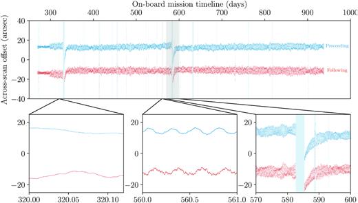
The across-scan distance between the locations of the two fields of view in our corrected scanning law and their locations in the nominal scanning law, in the frame of the nominal scanning law. This figure is comparable to fig. 3 of Paper I. The light blue bars in each panel indicate the gaps derived in Section 4, during which there are no published detections of variable stars.
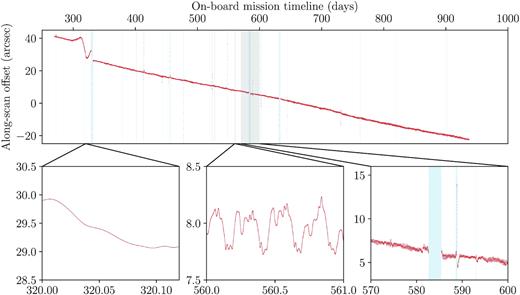
The along-scan distance between the locations of the two fields of view in our corrected scanning law and their locations in the nominal scanning law, in the frame of the nominal scanning law. The preceeding and following fields of view have identical along-scan offsets.
4 EFFICIENCY OF OBTAINING USEFUL DETECTIONS FROM OBSERVATIONS
If we had perfect knowledge of Gaia’s scanning law then we could predict the number of times that any star would have transited across either of the two fields of view, which we will term to be a predicted observation. Not every observation of a star results in a measurement in the Gaia DR2 variable star epoch table, which we will term to be a published detection. There are several reasons why a predicted observation might not result in a published detection:
Gaia experienced events which resulted in some detections not being of sufficient quality for publication in DR2 (e.g. the decontamination procedures or micro-meteoroid impacts, see Gaia Collaboration 2016). We term these periods to be gaps because no star of any magnitude has any published detections from during these periods. Part of the data taken during DR2 gaps may appear in subsequent DR.
An observation only results in a published detection with some probability which depends on the properties of the source. This may be because the occurrence of a detection is probabilistic (for instance, at the faint magnitude limit photon shot noise will result in stars being detected on only a fraction of their observations) or because of quality cuts made by the Gaia DPAC.
Gaia has a limited capacity to assign windows to stars and store and downlink the resulting scientific data, and so if densely populated regions are being scanned then only some fraction of the predicted observations will result in data that makes it to the ground. The retention behaviour is decided by magnitude bin (see Table 1), with some bins being prioritized to ensure good calibration across the entire magnitude range.
The magnitude bins used on-board by Gaia to determine priority for deletion if the downlink bandwidth is exhausted and which we used to bin the epoch measurements in this work. The first three columns of this table are a reproduction of table 1.10, section 1.3.3 of de Bruijne et al. (2018).
| Packet | Magnitude range | Deletion (per cent) | l (d) | ε (d−1) |
|---|---|---|---|---|
| SP1-1 | (5.00,13.00) | 0 | 150.49 | 1.53 |
| SP1-2 | (13.00,16.00) | 0 | 1.57 | 1.58 |
| SP1-3 | (16.00,16.30) | 1 | 9.65 | 1.48 |
| SP1-4 | (16.30,17.00) | 1 | 1.78 | 1.52 |
| SP1-5 | (17.00,17.20) | 2 | 7.01 | 1.52 |
| SP1-6 | (17.20,18.00) | 2 | 2.15 | 1.52 |
| SP1-7 | (18.00,18.10) | 2 | 11.11 | 1.51 |
| SP1-8 | (18.10,19.00) | 2 | 2.01 | 1.44 |
| SP1-9 | (19.00,19.05) | 2 | 7.02 | 1.30 |
| SP1-10 | (19.05,19.95) | 7 | 0.28 | 1.21 |
| SP1-11 | (19.95,20.00) | 2 | 7.87 | 1.00 |
| SP1-12 | (20.00,20.30) | 13 | 1.39 | 0.99 |
| SP1-13 | (20.30,20.40) | 12 | 2.32 | 1.08 |
| SP1-14 | (20.40,20.50) | 13 | 2.21 | 1.07 |
| SP1-15 | (20.50,20.60) | 28 | 2.51 | 1.02 |
| SP1-16 | (20.60,20.70) | 28 | 3.01 | 0.97 |
| SP1-17 | (20.70,20.80) | 28 | 8.64 | 0.84 |
| SP1-18 | (20.80,20.90) | 28 | 19.67 | 0.73 |
| SP1-19 | (20.90,21.00) | 24 | 15.10 | 0.63 |
The objective of this section is to rigorously identify the gaps in Gaia data taking by exploiting the DR2 variable star epoch photometry. We attempted this in Paper I by looking for periods longer than 1 per cent of a day where none of the variable stars had a published detection, but there were several possible issues with this approach. First, this approach cannot distinguish between a period with no published detections and a period where no variable stars were observed because Gaia was scanning a sparse region of the sky. Second, our choice of 1 per cent of a day was an attempt to mitigate the first problem and it is likely that there are gaps shorter than this. Third, gaps are not the only reason that an observation might not result in a detection, as mentioned above.
Our novel methodology in this work is based on the idea that a run of non-detections could be due to a gap or it could be due to those stars having a low probability that an observation would result in a published detection. By pairing the published detections with the predicted observations that failed to result in published detections and weighing the possibility of a gap against the possibility of low detection efficiencies, we are able to search for gaps in a way that is robust to the density of variable stars on the sky and to the low detection efficiency of faint stars. We model the probability of a source with magnitude G having a published detection at the predicted observation time t as A(t)B(G, t), where A(t) takes binary values and represents gaps that affect all magnitudes equally while B(G, t) can take any value in (0,1) and represents any other effects that can cause an observation to not yield a published detection. We assume that the magnitude dependency of B(G, t) is piecewise constant such that at time t it takes a different value in each of the star packet magnitude intervals (see Table 1), because one of the most important drivers of a time-varying detection probability is crowding and the impact of crowding changes between each star packet magnitude interval.
In Section 4.1, we discuss the preparation of the data and the prediction of the times of observation. We describe our discrete hidden Markov model for A(t) in Section 4.2 and our extended Kalman filter model for B(G, t) in Section 4.3. The full Bayesian specification of this problem would require us to have a posterior over millions of parameters (one discrete and one continuous hidden state at each epoch measurement in addition to the tens of hyperparameters) and so we opt for an iterative maximum-likelihood approach which we describe in Section 4.4.
4.1 Predicting observations and data cleaning
We use the 550 737 variable stars in the Gaia DR2 epoch photometry tables. We extract the times of observation at Gaia from the transit_id and approximate the error in the epoch G magnitude from the reported epoch flux and flux error. For each source in the epoch photometry table we then predict when it would have been observed during the 22 months of Gaia DR2, following the methodology laid out in Papers I and II and using the scanning law derived in Section 3. The resulting 19 685 650 predicted observations were then matched to the published detections with a window of |$1{{\ \rm per\ cent}}$| of a day, with the predicted observations being assigned a value of one if they are matched with a published detection and zero otherwise.
Our methodology is magnitude dependent and so we must assign a magnitude to each predicted observation. In the case of those with matching published detections, we take the magnitude estimate and error reported at that epoch, but for the non-detections we must infer the magnitude at those epochs. The naïve approach would be to assign the mean G-band magnitude from the Gaia source table to be the magnitude at each non-detection, but that ignores that these stars have been identified to be variable stars and thus the magnitude will significantly change between epochs. The best way to proceed would be to have theoretical models that predict the light curves of different types of variable star objects, fit those model light curves to the published detections in a Bayesian way, and then marginalize over those fits to obtain a predicted measurement at each of the predicted observations without a published detection. However, this is far beyond the scope of this work and would likely only make a marginal difference to our results. We will be combining the measurements from many stars into magnitude bins and thus a few observations crossing the border into an adjacent magnitude bin should not overly bias our results. We therefore decided to infer these values using Gaussian process regression, to which we gave an introduction in Section 2.1. The reader should view our use of Gaussian process regression in this instance as a mathematically convenient curve-fitting scheme that can account for uncertainty in the individual magnitude measurements.
We assume that the time evolution of the magnitude of each star can modelled as the realization of a Gaussian process. We have measurements of the magnitude G(ti) and magnitude variance σ2(ti) at times |$\lbrace t_{i}\rbrace _{i = 1}^{n}$| and wish to predict the magnitude at any time t*. We assume that the mean is constant, and that the covariance kernel is given by equation (3). We fix the mean and signal variance according to equations (7) and (8). Though the actual period distribution of the published variables stars ranges from hours till hundreds of days, we fix the length scale to l = 1 d as a very rough ‘typical’ value. This has the consequence that a non-detection occurring soon before or soon after a detection will be assigned a magnitude close to that of the detection, whereas a non-detection occurring long before or long after a detection will be assigned a magnitude close to the sample mean. The scanning law causes most stars observed in the preceding field-of-view to be observed 2 h later by the following field of view and thus observations come in pairs. Our inference scheme is therefore most effective in the fairly common case that one of these observations did not result in a detection. We give examples of the use of Gaussian process regression to infer the magnitudes of non-detections in Fig. 4.
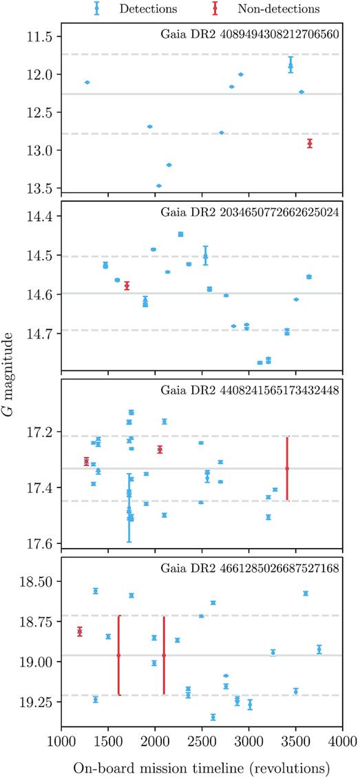
Examples of the results from our use of a Gaussian Process to impute the magnitudes of the variable stars at the epochs at which they were predicted to be observed but that did not result in a published detection in the Gaia DR2 epoch photometry tables. The solid and dashed lines indicate the weighted mean and 1σ regions of the published detections of each star.
We applied this formalism to all 550 737 of the stars with epoch photometry. We then used the magnitude at each predicted observation to group them across all stars by magnitude into the bins given in Table 1, and further sorted these observations by time. If there is a matching published detection then the magnitude used for the grouping is the one measured by Gaia, otherwise it is the magnitude infilled by our Gaussian Process as described above.
In summary, we have magnitude bins i = 1, …, 19 each with a time-series |$t_j^i$| of predicted observations j = 1, …, Mi each with a flag |$k_j^i$| which indicates whether there is a matching published detection (|$k_j^i=1$|) or not (|$k_j^i=0$|).
4.2 Hidden Markov Model for gaps
4.3 Continuous state space modelling
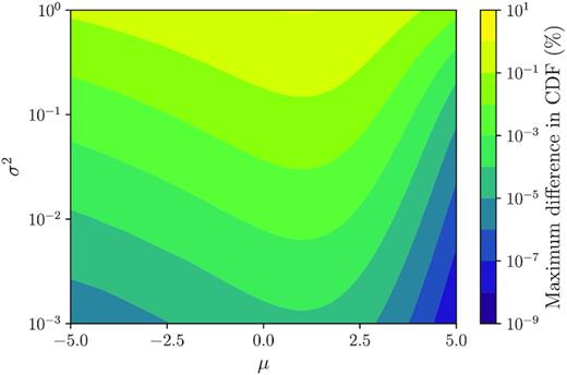
The maximum percentage difference between the cumulative densities of the function Φ(x)ϕ(x|μ, σ2) and the Gaussian approximation described in the text.
We need to obtain both the likelihood of the hyperparameters l and ε2 and the best estimate of the states |${X_i}_{i=1}^{n}$| given the observations |${Y_i}_{i=1}^{n}$|. The reason our model cannot be expressed as a conventional extended Kalman filter is that our observations are not continuous and thus we cannot simply differentiate the observation model with respect to the state space parameters. We instead follow the formalism laid out in Fraser (2008, chap. 4).
If there is known to be a gap at time ti, then we adjust the expressions above by stating P(yi|xi) = 1.
4.4 Estimating the hyperparameter likelihood and discussion
Our model for the gaps has two free parameters q and r and our model for the detection efficiency has two free parameters li and |$\varepsilon _i^2$| in each magnitude bin i, for a total of 38 free parameters. The run-time of both algorithms is linear in the number of predicted observations and thus it would be prohibitively expensive to simultaneously optimize all parameters. We opt instead to alternate between optimizing the free parameters in the gaps model and optimizing the free parameters in the detection efficiency model, using the maximum-likelihood gaps or efficiencies from the last optimization of each in the next optimization of the other.
Our final time-scales for the persistence of non-gaps and gaps were q = 1.216 and r = 0.043 d. If the time between the current state and the next is equal to the persistence time-scale then the probability of the next state being the same as the current state is 68.4 per cent, while if the time difference is twice the persistence time-scale then the probability of remaining in the same state is only |$56.8{{\ \rm per\ cent}}$|. Our final values for q and r tell us that gaps are not frequent and tend to be short-lived. The final values for the time-scale l and variance ε2 of the detection efficiency process in each magnitude bin are given in Table 1. These describe the time-scales over which the detection efficiencies appear to vary and the scale of those variations. We illustrate the final gaps and detection efficiencies in Fig. 6.
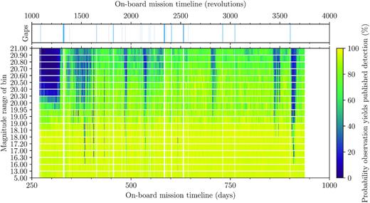
Illustration of our final gaps and probabilities of detection. Top: the inferred gaps where no Gaia observations resulted in published detections are shown in blue. Bottom: for each of the magnitude bins used to define Gaia star packets, the colour map shows the probability that a Gaia observation made at that time would result in a published detection.
Fig. 6 shows rich structure which can be attributed to known effects. The drops in detection probability around |$\mathrm{OBMT}\, 1925\,\,\mathrm{rev}$|, 2150 rev, 2825 rev, 3475 rev, and 3575 rev are due to periods when Gaia was frequently scanning across the Galactic plane. The initial period of low detection probability for sources fainter than G = 20.3 is due to the faint-end threshold for the SkyMapper CCDs to register a detection (de Bruijne et al. 2015) originally being set to G = 20.3. This threshold was changed to G = 21.0 on 2014 September 15 and decreased to its final value of G = 20.7 on 2014 October 27 (see section 1.3.3 of de Bruijne et al. 2018). These threshold changes do not appear as crisp edges in this plot because the SkyMapper-estimated G magnitude is not as accurate as the calibrated measurement made by the astrometric CCDs. We identified a total of 206 gaps, an increase from the 94 gaps identified in Paper I. The gaps which are clearly visible in Fig. 6 were primarily caused by the mirror decontaminations and subsequent refocusings, station-keeping maneuvers, and micro-meteoroid impacts.
5 USING OUR SCANNING LAW TO PREDICT GAIA OBSERVATIONS AND THE PROBABILITY OF THEM RESULTING IN DETECTIONS
The results of our series of papers rely heavily on predicting when Gaia observed a location on the sky, given the scanning law. Being able to predict Gaia observations would be useful in other science cases beyond inferring Gaia’s completeness, and so we have produced a python module scanninglaw (https://github.com/gaiaverse/scanninglaw) based on the dustmaps package by Green (2018) and subsequent selectionfunctions package from Paper II. This enables the user to ask the question ‘At what times could Gaia have observed my star in the time frame of DR2 and what is the probability that each observation was successfully processed?’. This is demonstrated by determining when the fastest main-sequence star in the Galaxy (S5-HVS1, Koposov et al. 2020) would have been observed in Gaia DR2. This python package has options to download and use the DPAC nominal scanning law or the one derived in Section 3 of this work.

6 CONCLUSIONS
The completeness of the Gaia catalogues is heavily dependent on the status of Gaia through time. If there is a gap in scientific operations, a drop in the detection efficiency or Gaia deviates from the commanded scanning law, then stars will miss out on potential detections and thus be less likely to make it into the Gaia catalogues. The Gaia mission will take hundreds of epoch astrometric, photometric, and spectroscopic measurements of billions of stars, which will implicitly encode the status of Gaia throughout the mission. In this work, we have laid the groundwork for the future exploitation of these massive time-series by developing novel methodologies to infer the orientation of Gaia and the gaps and detection efficiencies from time-series of Gaia detections. We have applied these methodologies to the Gaia DR2 variable star epoch photometry which are the only publicly available Gaia time-series at the present time. The nominal scanning law will be updated in the early third Gaia DR3, but the true attitude determination used in the DPAC astrometric solution will not be made available at that time.4 Therefore, in a later paper in this series we will determine a more accurate scanning law for the period covered by DR3 by applying the methods presented in this paper to the extended variable star photometry which will become available in the full DR3.
The objective of this work in the context of the Completeness of the Gaia-verse series was to more accurately infer Gaia’s true scanning law and the timings of data-taking gaps, which will be used in subsequent works to infer selection functions for the astrometric, photometric, and spectroscopic data products. However, our results are also of immediate practical use. We have created a new open-source python package scanninglaw which can be used to query the times that Gaia observed a location on the sky and the probability of each of those observations resulting in a published detection. This package can download and use any of the publicly available scanning laws for the 22 months of Gaia DR2.
ACKNOWLEDGEMENTS
DB thanks Magdalen College for his fellowship and the Rudolf Peierls Centre for Theoretical Physics for providing office space and travel funds. AE thanks the Science and Technology Facilities Council of the United Kingdom for financial support. This work has made use of data from the European Space Agency (ESA) mission Gaia (https://www.cosmos.esa.int/gaia), processed by the Gaia Data Processing and Analysis Consortium (DPAC, https://www.cosmos.esa.int/web/gaia/dpac/consortium). Funding for the DPAC has been provided by National Institutions, in particular the institutions participating in the Gaia Multilateral Agreement.
DATA AVAILABILITY
The data underlying this article are publicly available from the European Space Agency’s Gaia archive (https://gea.esac.esa.int/archive/). The scanning law derived in Section 3 is publicly available on the Harvard Dataverse (https://doi.org/10.7910/DVN/MYIPLH), as are the identified gaps and detection probabilities in Gaia data-taking (https://doi.org/10.7910/DVN/ST8TSM). The authors welcome queries from those interested in using our data products in their own works.
Footnotes
Note that Gaia does not use any gyroscopes to guide its attitude, instead it uses a cold-gas micro-Newton thruster system firing several times per second, using the scientific instrument measurements to maintain the programmed scanning law during nominal operations (Gaia Collaboration 2016).
An analogy can make this clearer. Imagine we release a satellite on a circular orbit about the Earth and at the same time release a second satellite on a slightly inclined but otherwise identical orbit. The distance between these two satellites will oscillate with a period that is identical to the period of their orbit. Similarly, small offsets in the estimated angular velocity of Gaia between the nominal scanning law and our derived scanning law cause the angular offset between the two to oscillates with Gaia’s rotation periods.
