Circular polarization in radio pulsar PSR B1451−68: coherent mode transitions and intrabeam interference Free

ABSTRACT

1 INTRODUCTION

Studies of pulsar polarization have a half-century-long history, with publications addressing many different aspects: the appearance of observed average polarization at different frequencies (Karastergiou & Johnston 2006; Hankins & Rankin 2010; Dai et al. 2015; Noutsos et al. 2015), various statistical and instrumental effects (McKinnon & Stinebring 1998), propagation effects in the interstellar medium (Karastergiou 2009), single-pulse polarization (Smith, Rankin & Mitra 2013; Mitra, Arjunwadkar & Rankin 2015), and others. Theoretical works involved recognition of basic magnetospheric geometry (RVM, i.e. the rotating vector model; Radhakrishnan & Cooke 1969; Komesaroff 1970), polarization of curvature radiation (CR; Michel 1991; Gangadhara 2010), calculations of allowed magnetospheric propagation modes (Melrose & Stoneham 1977; Arons & Barnard 1986), analytical modelling of propagation effects (Petrova & Lyubarskii 2000), numerical ray tracing with propagation effects (Wang, Lai & Han 2010; Hakobyan, Beskin & Philippov 2017), and empirical modelling of circular polarization. The latter was based on either coherent mode superposition (Kennett & Melrose 1998; Edwards & Stappers 2004) or the non-coherent superposition of modes (Melrose et al. 2006).

In this paper, we study the variations of circular polarization in PSR B1451−68 (PSR J1456−6843) and the associated flow of radiative power between orthogonal tracks of polarization angle (PA). The transition of radiative power between the orthogonal PA tracks naturally occurs in a model that assumes that the observed polarization state (i.e. a point or patch on the Poincaré sphere) results from a coherent superposition of orthogonally and linearly polarized¹ proper mode waves. As described in Dyks (2017, hereafter D17), whenever the waves have similar amplitudes and combine at a phase lag of |${\sim}90^\circ$|⁠, the orthogonal transitions occur in coincidence with maxima of circular polarization (see figs  11, 12, and 13 therein). This can happen in various physical situations: (1) when the phase lag distribution keeps extending up to 90^○ and the amplitude ratio is changing with pulse longitude Φ (fig. 11 in D17); (2) when similar-amplitude waves are coherently summed at a longitude-dependent phase lag (figs 12 and 13 in D17); (3) when both the amplitude and lag are longitude dependent (fig. 23 in Dyks 2019, hereafter D19). It has been found that identification of a single strong PA track with a single RVM curve is in general meaningless (section 4.3.1 in D17). Indeed, some observations prove that the RVM tracks are hard to identify without earlier recognition of polarization modes (Mitra & Rankin 2008).

Transition through the state of quarter-cycle lag at similar wave amplitudes has a simple representation on the Poincaré sphere, where it corresponds to the passage near or through the V pole. The passage occurs during a near-meridional rotation of polarization state on the Poincaré sphere. The earliest illustration of this phenomenon can be found in the PhD thesis of Ilie (2019) where the V pole passage (VPP) can be seen directly on Poincaré sphere maps (B1451−68, fig. 3.45 therein). Ilie’s thesis also presents distributions of ellipticity angle |$\kappa = \frac{1}{2}\arctan (V/L)$|⁠, where V and L are the observed circularly and linearly polarized fluxes, respectively. This makes it possible to recognize the VPP effect even without the help of Poincaré sphere projections (e.g. PSR J1900−2600, fig. 3.64 in Ilie 2019).

Whatever is the physical reason, the passage of polarization state through the V pole is a transition to an opposite azimuth on the Poincaré sphere, and the opposite azimuth means orthogonal PA (see figs 2 and 3 in Dyks 2020, hereafter D20). Moreover, because of its near-polar nature, when mapped on the traditional longitude–PA diagram, the VPP phenomenon produces several polarization artefacts that result from the usual cartographic problems of circumpolar mapping (D20). For example, PA track bifurcations and vertical spread of PA result from immersion of the V pole within the modal patch. Excessive span of PA observed on the equatorward side of star’s magnetic pole can also result from the traverse of flux patch near the V pole of Poincaré sphere.

In this paper, we analyse Ilie’s data on PSR B1451−68 in more detail (Section 2). Then we derive analytical formulae that allow us to describe arbitrary rotations of the polarization state on the Poincaré sphere. In Section 4, the meridional circularization in B1451−68 is interpreted as a coherent orthogonal polarization mode (OPM) transition. In Section 5, the VPP OPM transitions are calculated numerically to present the mapping from the Poincaré sphere in the case of similar strength of both modes. Some of the model results are identified in the polarization of B1451−68. A possible geometric origin for the mode strength imbalance between the leading and trailing sides of the profile is discussed in Section 6. Then we try to use the symmetry properties to constrain possible physical interpretations of polarization observed in B1451−68 (Section 7). This leads to a model of pulsar emission that is based on four-mode interference (Section 8).

2 OBSERVATIONS AND POLARIZATION CHARACTERISTICS

2.1 Observations

PSR B1451−68 (J1456−6843) was observed in 2016 with the Parkes telescope within a survey of modulated radio pulsar polarization (chapter 3 of Ilie 2019). In total, 8755 consecutive single pulses were recorded at a central frequency of 1369 MHz with a bandwidth of 256 MHz. The acquired polarization data on PSR B1451−68 are analysed using psrsalsa  ² (Weltevrede 2016) and are shown in Fig. 1 (reproduced fig. 3.44 of Ilie 2019). Panel (e) presents the greyscale distribution of PA as measured in single samples as a function of pulse longitude Φ. Two similarly strong PA tracks that follow the RVM are visible. Both these near-orthogonal PA tracks (upper and lower) consist of three sections marked A, B, and C. The sections are separated by breaks, i.e. longitude intervals where the PA is spread vertically over a large range of values; hence, the greyscale histogram becomes pale there.

Figure 1.

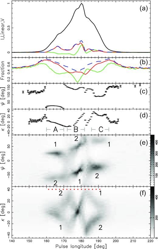
Polarization of PSR B1451−68 at 1369 MHz (after Ilie 2019). (a) Average profile with total (black), linear (red), circular (green), and total (blue dashed) polarization. (b) Arithmetic average of instantaneous polarized fractions: total (dashed), linear L/I (red), and circular |V|/I (green). Only samples for which the total polarization, L and V, exceeds the off-pulse r.m.s. are included in the average. (c) Average PA. (d) Average ellipticity angle. (e) Histogram of PA measured in single samples for which L exceeds the off-pulse r.m.s. (f) Histogram of ellipticity angle measured in single samples for which the total polarization exceeds the off-pulse r.m.s. The numbers in (e) and (f) refer to different OPMs (different patches on the Poincaré sphere shown in Fig. 2). Three regions of interest are labelled in (d). The dots in panel (f) refer to the pulse longitudes explored in more detail in Fig. 2.

Open in new tabDownload slide

The ellipticity angle κ, shown in the bottom panel, forms a bow tie shape. The radiation of both modes is linearly polarized on the leading side of the profile (κ ∼ 0, Φ = 160^○), then κ approaches ±45^○, crosses zero in the middle of the profile (longitude 178^○), and again reaches ±45^○ before becoming nearly linear on the trailing side.

2.2 Poincaré sphere view

The behaviour of polarization in PSR B1451−68 becomes clear when the data are plotted on the Poincaré sphere (P. sphere). Fig. 2 illustrates distributions of the polarization state on the P. sphere for 15 longitudes (a different set of six longitudes is shown in fig. 3.45 of Ilie 2019). Each distribution consists of samples recorded in different rotation periods and it has the form of two approximately antipodal flux patches on P. sphere. Hereafter, these are called ‘patches’ whereas the term ‘modes’ is reserved for the linear proper modes in high magnetic field. The question of when and whether the patches correspond to the proper modes or represent a mixed state will be resolved in Section 4. Fig. 2 implies that the patches are rotating almost meridionally on the P. sphere, with each flux patch passing near each V pole (northern and southern, i.e. positive and negative V). This gives four near-pole transitions that correspond to the four peaks at κ ∼ ±45^○ in the bow tie curve of the ellipticity angle (panel f of Fig. 1).

Figure 2.

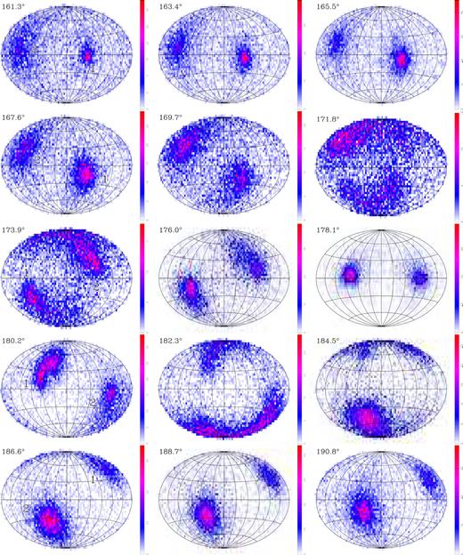
Histograms of polarization states observed at the longitudes shown in the top-left corner of each panel and marked with red dots in Fig. 1(f). Each map presents Hammer equal area projection of Poincaré sphere. In the left-hand panels, the model patches are labelled consistently with the bottom panels of Fig. 1.

Open in new tabDownload slide

Figure 3.

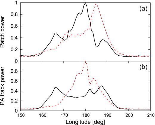
Top: normalized polarized flux integrated within each patch on the P. sphere. The solid line corresponds to patch 1 (mode 1). Bottom: normalized polarized flux integrated within each RVM-like track of PA. The solid line is for the top track in Fig. 1(e).

Open in new tabDownload slide

The labelling of the patches on the P. sphere corresponds to those in the bottom two panels in Fig. 1. The stronger (primary) patch (no. 1) forms the upper PA track at the leading side of the profile, but with increasing pulse longitude this patch moves downwards on the P. sphere. After passing near the southern V pole, the flux of patch 1 forms the bottom PA track (interval B in Fig. 1). Therefore, the upper PA track is stronger in interval A, whereas the lower track is stronger in interval B. In the middle of interval B, the patches pass through the equator (κ ∼ 0), then they continue near-meridionally polewards, and pass near the V poles while entering the interval C. Therefore, the flux patch with no. 1 forms the peripheric parts of the upper track while the track’s centre corresponds to patch no. 2. Opposite arrangement holds for the lower PA track (see the patch numbers in Fig. 1). In the bottom panel in Fig. 1, patch 1 corresponds to the ‘down–up–down’ branch of the bow tie, whereas patch 2 corresponds to the ‘up–down–up’ branch.

The ±45^○ tips of the bow tie coincide in longitude with the breaks in the PA tracks, which is consistent with the VPP. The transition between intervals A and B seems to exhibit an X-shaped feature: The upper track PA decreases towards the lower track, whereas the PA of the lower track increases towards the upper track, so that the tracks cross each other at the transition. Another transition – between intervals B and C – looks as a pale break in the tracks, with the PA of a given track splitting both upwards and downwards. This is most clearly seen on the left side of interval C for the lower track.

The lower two panels of Fig. 1 allow us to follow the strength (frequency) of each patch separately. The branches A1 and B1 are consistently stronger than A2 and B2, which is consistent with the VPP and the transfer of flux between orthogonal PA tracks (see fig. 2 in D20).

On the trailing side of the profile, however, at the B–C transition, branch C2 becomes stronger than C1; i.e. patch 2 becomes stronger than patch 1. The coincidence of the bow tie tips at the B–C transition with the breaks in the PA tracks leaves little doubts that the near-pole passage has occurred at Φ ≈ 183^○. Therefore, the radiative power of patch 1 must have been transferred from the lower to upper PA track at the B–C transition. The large strength of the C2 branch can thus only be explained by the simultaneous inversion of the patch flux ratio; i.e. patch 2 becomes stronger than patch 1 on the trailing side of the profile (within interval C).

It is therefore concluded that the inversion of power in the different parts of PA track can occur in two different ways: either through the VPP (whereby the power ratio in PA tracks is inversed, but not the ratio of the patch flux content) or through the actual (real) change of power content, i.e. in each patch on the P. sphere. In PSR B1451−68, the patch power inversion appears to coincide in longitude with the VPP at the B–C transition. This is meaningful, because the equal power (amplitude) of near-orthogonal waves is necessary for their combination to produce the pure V polarization state.

The described behaviour is further complicated by the fact that the patches tend to assume an extended arc form near the V poles. Therefore, while passing through the V pole, a single elongated patch can persist for a long time on opposite half-meridians; i.e. near the OPM transitions, a single patch can contribute to both orthogonal PA tracks ‘simultaneously’ (i.e. at a fixed longitude).

Moreover, near the profile centre (interval B) the modal patches assume a double or bifurcated shape, thus forming four subpatches. In Fig. 2, the double form is clearly visible for the weak (right) patch 2 at Φ = 176^○ and for the bright (left) patch 1 at Φ = 180.2^○. Each subpatch moves at a different speed in different directions on the P. sphere in such a way that the subpatches coincide when crossing the equator, i.e. near the central profile minimum at Φ = 178^○. Because of this longitude-dependent bifurcation, each PA track in the centre of Fig. 1(e) (interval B) is split into two subtracks with different PA slopes.

The shape-related complexities (extensions or bifurcations of patches) are addressed in Section 4.4.

2.3 Profiles of separate polarization modes

The power content of a given polarization mode can be defined as the flux belonging to a given patch instead of the flux contained in a given RVM-like track of PA. Fig. 3 presents mode-separated profiles calculated according to these two definitions. The solid and dashed lines in the top panel present the polarized flux of patches 1 and 2, respectively. These are determined by integrating the polarized flux within each of the hemispheres of the P. sphere after placing the centre of the brightest patch at the pole. One can see that most of the polarized power in the trailing side of the pulsar’s profile is associated with patch 2. It is also evident in Fig. 3(a) (as well in Fig. 2) that patch 2 also becomes slightly stronger during the first V passage. Overall, the polarized profile of patch 2 (dashed) looks like a time-delayed version of the patch 1 profile (solid), although there is no third trailing component in the former. Interestingly, two peaks in the flux profiles of different patches have nearly identical height. The patch-based mode separation produces profiles with a characteristic anticorrelation, which is also observed in the modulation patterns of pulsars (Deshpande and Rankin 2001; Ilie et al. 2020).

The bottom panel of Fig. 3 presents the polarized flux integrated within each PA track, i.e. within ±45^○ from an RVM fit. Such mode separation is similar to the three-way mode segregation of Deshpande & Rankin (2001). The method produces completely different mode-segregated profiles than the patch-based method: The top PA track (solid line) has a double form that does not dominate in the profile centre.

The question on which panel of Fig. 3 represents the correct mode separation depends on the physical origin of the VPP effect. If the rotating patches correspond to elliptic proper OPMs, then Fig. 3(a) is appropriate. If, however, the rotating patches only represent a mixed state that results from the coherent superposition of linear proper modes, then Fig. 3(b) applies. In the latter case, the VPP just represents a coherent OPM jump; i.e. the proper polarization states do not pass near the V poles. In Section 4, we show that the coherent OPM jump is the correct interpretation. This implies that adjacent profile components have to consist of linear orthogonal modes with appropriate phase lag difference (see Section 7.2).

2.4 Polarization fractions and similarity to PSR B1237+25

Fig. 1(b) shows that near the V poles (Φ = 172^○ and 183^○) the instantaneous polarization degree is typically quite high (I_pol/I ≈ 0.5–0.6). Therefore, the incoherent mode superposition (Melrose et al. 2006) is not responsible for the observed VPP (though it is at work in other objects).

The ‘typical instantaneous’ polarization fractions reveal a quite symmetric form, with twin minima in L/I flanking the maximum of the core component. The minima coincide with peaks of |V|/I that also has a quite symmetric form. These curves reflect the near-meridional rotation of polarization state, which produces the anticorrelation between L/I and |V|/I.

Thus, regarding the typical instantaneous polarization fractions, the pulsar B1451−68 resembles the well-known ‘complex core’ pulsar B1237+25, for which the V-coincident twin minima have also been observed and interpreted through the rotation of the polarization state (D17; D20). In B1237+25, however, the features are visible in the standard Stokes-averaged fractions, probably because of larger disproportion of OPMs’ power. In the case of B1451−68, the standard Stokes-averaged polarized fractions have complex longitude dependence and do not exhibit any clear symmetry (so we do not show them in this paper).

3 ANALYTICAL FORMULAE FOR VPP

In this section, we introduce the equations for the rotation of a pol. state on Poincaré sphere. It is shown that the rotation implies essentially the same PA curve as the RVM. In the following Section 4, it is shown that the rotation is caused by the coherent orthogonal mode transition, i.e. by variations of the ratio of mode amplitudes. Coherent OPM jumps do not necessarily involve the decrease of the linear polarized fraction. Therefore, several OPM jumps have been misinterpreted as RVM and many of them might have been missed in pulsar data (Section 4).

The rotation of the polarization state on the Poincaré sphere may reflect intrinsic properties of the emission or it may directly result from a coherent superposition of orthogonally polarized waves that oscillate at some relative phase lag. Regardless of the actual origin, the patch rotation can be mathematically considered as a retarder action on the Poincaré sphere, with the rotation angle corresponding to the phase lag. The purely meridional patch motion (meridional circularization) may in particular correspond to a linear retarder action, with the polarization state rotating around the axis contained in the equatorial plane (Q–U plane). Physically, this may correspond to the O-mode retardation (Edwards & Stappers 2004; Jones 2016; D17). Aside from this mechanism, the meridional circularization may also correspond to a coherent OPM transition (COMT; inversion of mode amplitude ratio at a fixed phase lag, in this case of quarter-wave length).

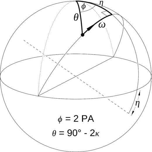
Before introducing a general case, this section deals with two simple limiting cases of pole passage: (1) Rotation of arbitrary polarization state around an equatorial axis (linear retarder; see Fig. 4). Here, the arbitrariness of polarization state implies that motion along small circles is allowed, i.e. the angle between the polarization state and the rotation axis may be arbitrary. (2) Great-circle rotation around a non-equatorial axis (coherent OPM jump, i.e. transition between two antipodal modes; also a retarder with elliptical proper modes). In this case, only the motion along a great circle is considered (see Fig. 5). Finally, the two cases are combined in a general case of rotation in arbitrary circle (i.e. small or great) around an arbitrary rotation axis.

Figure 4.

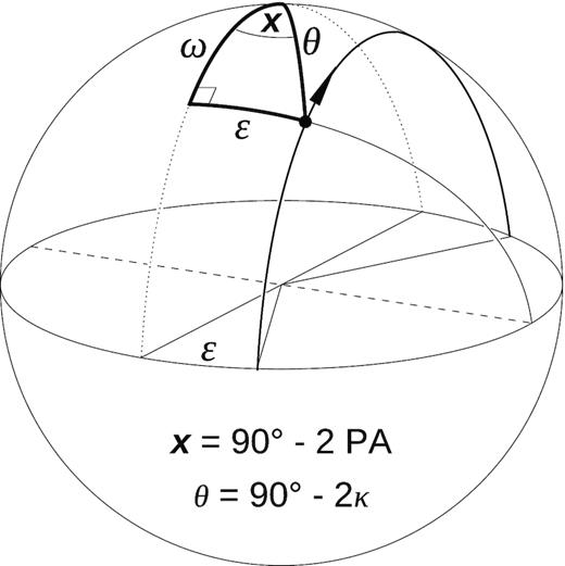
Geometry of the near-meridional circularization on the Poincaré sphere in the case of linear retarder axis (equatorial axis of patch rotation, dashed diameter). The polarization state (flux patch on the Poincaré sphere) moves along the thick circle parallel to the dotted meridian. The position of the state is parametrized by the angle ω. The thick spherical triangle is used to derive equations (4) and (5).

Open in new tabDownload slide

Figure 5.

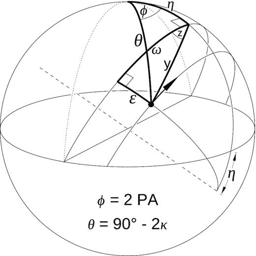
Geometry of near-meridional circularization in the case of an arbitrary axis of patch rotation (dashed diameter). The polarization state (bullet) moves along the thin solid great circle and the states’ position is parametrized by the angle ω. The thick spherical triangle is used to derive equations (6) and (7).

Open in new tabDownload slide

3.1 Linear retarder, arbitrary polarization state

Equation (4) describes the passage of radiative power from one PA track to the other, near-orthogonal PA track. Thus, equation (4) is followed during an OPM jump when the jump is caused by the VPP. This equation has the geometric form of an S-shaped function; therefore, an observed OPM jump caused by the VPP can be mistaken for the RVM S swing.

3.2 Coherent OPM jump at a fixed phase lag; elliptical retarder with great-circle rotation

In the case of elliptical proper modes, the patch is rotated around an arbitrarily oriented axis (dashed diameter in Fig. 5). Here, the axis is tilted by an arbitrary angle η with respect to the V axis. The PA ψ = ϕ/2, where ϕ is the azimuth (Fig. 5). Again, the value of ψ is the PA value as measured with respect to the PA of the patch rotation axis, i.e. ψ_obs = ψ + ψ_RVM + ψ₀.

As explained in Section 4, the rotation geometry of Fig. 5, i.e. the great-circle rotation between antipodal points, also refers to the mode-ratio-driven COMT; however, in the COMT case the proper mode axis corresponds to the solid diameter in Fig. 5 and the modes are linear, not elliptic. The mode strength ratio and phase lag δ_ox correspond to different angles in Fig. 5 than in the case of retardation (see Fig. 7 and Section 4).

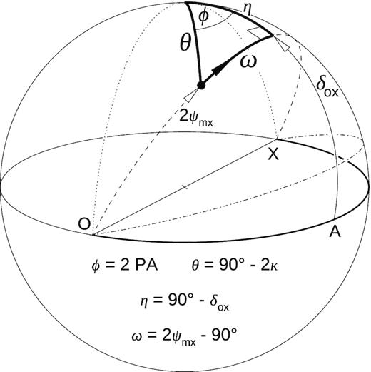
3.3 General case: arbitrary-circle rotation around arbitrary axis

Figure 6.

Geometry of circularization in the case of arbitrary polarization state (bullet) and arbitrary axis of the state’s rotation (dashed diameter). The derivation of equations (9) and (8) makes use of the two thick spherical triangles: (θ, η, y) and (ϵ, ω, y), where the shared side y cancels out in the process.

Open in new tabDownload slide

As before, some observed S-shaped variations of PA may be mainly caused by the VPP rather than by the RVM. This may happen when the VPP variations of PA are much faster than RVM; i.e. the RVM curve is relatively flat. In such case, the S swing should be modelled with equation (9). When the RVM-driven changes of PA are also noticeable, equation (10) needs to be used.

4 COMT

4.1 Coherent OPM jump or retardation?

The main possible interpretations of the meridional circularization involve the retardation of the O mode and the COMT. In the case of linear proper modes, the increase of the phase lag δ_ox between the X and O mode causes the rotation of the summed polarization state around the equatorial QU axis (Fig. 4). The lag is changing along with the ω angle: δ_ox = 90^○ − ω. If the amplitudes of the modes E_X and E_O are equal, the bullet follows the meridian that is orthogonal to the dashed proper mode axis (ϵ = 0). Otherwise, ϵ = 90^○ − 2ψ_mx, where tan ψ_mx = E_O/E_X is the mixing angle. A spread of phase lags results in a spread of polarization state vectors in the meridional direction, which seems consistent with the patch extension along the meridian, as observed near the V poles. However, this is the only feature that may be considered consistent with the observations, whereas multiple arguments can be put against the retardation.

First, the meridional retardation requires that the mode strength stays equal throughout the entire phenomenon, whereas the mode ratio is typically variable in pulsar signal (both in pulse longitude and in modulation phase).

Secondly, when the patches are far from the QU equator, we never observe the proper polarization states separately. If observed alone, the modes would produce two additional flux patches in directions orthogonal to the bullet motion plane (i.e. at the tips of the dashed diagonal in Fig. 4).

Thirdly, in the course of the increasingly strong retardation, the observed polarization state (bullet in Fig. 4) is always a mixed state: It is produced by the coherent superposition of the proper modes O and X. The bullet never coincides with the X or O mode. Contrary to this fact, the patches observed in B1451−68 become very compact while crossing the QU equator, which can be understood as a coincidence of the observed patches with the linear proper modes (transition from a mixed to the pure polarization state – see below).

Fourthly, if the phase lag δ_ox is acquired through propagation in birefringent medium, then, given the tubular symmetry of the polar region, it is natural to expect that δ_ox is a non-monotonic function of Φ, e.g. δ_ox could reach a maximum in the middle of the profile and vanish at the profile edges. In contrast to this expectation, the bow tie form of the polarization in B1451−68 clearly implies that the retarder rotation angle is steadily increasing across the full pulse window (from, say, δ_ox = 0, through 180^○, up to almost 360^○). The modal patches never stop rotating (as expected when the phase lag reaches maximum) nor they move backwards, as expected when the birefringent medium becomes rarefied towards the edges of the profile. Such lack of mirror symmetry could possibly result from ray propagation at high altitudes, but the simplest model based on the retardation cannot explain these observations.

It is therefore concluded that the meridional circularization is caused by the COMT.

4.2 COMT

Figure 7.

Geometry of the COMT on the P. sphere. The change of mode ratio corresponds to the change of mixing angle ψ_mx. For a constant phase lag δ_ox, the polarization state (bullet) follows a great circle tilted at the angle δ_ox with respect to the QU equator. The state can move meridionally through the V pole (δ_ox = 90^○ + n180^○) or equatorially through the A point (δ_ox = n180^○).

Open in new tabDownload slide

If δ_ox ∼ 90^○ + n180^○, the bullet follows the meridional path (dotted vertical in Fig. 7). This involves the VPP at ψ_mx = 45^○ associated with the OPM transition between the PA tracks. This type of quarter-wave OPM jump can be recognized by the very high |V|/I ≫ L/I coincident with minima in L/I (both observed at the longitude of the OPM jump).

During the meridional motion, the PA stays constant until the pole is passed by. Therefore, the corresponding PA curves are flat between the VPP OPM jumps. In case of two OPM jumps (e.g. on both sides of a core component), the PA tracks can have the shape of stairs (two upward OPM jumps or two downward), the U shape (downward and upward OPM jump), or a reversed U shape (jump up and down). Given that this quarter-wave OPM transition, as any COMT, is described by the RVM-like equation, the jump can sometimes be mistaken with the RVM; see the next section for examples.

If the lag δ_ox does not precisely have the quarter-wave value, the pol. state can move along the dashed line in Fig. 7. This corresponds to a PA curve that has the shape of stairs with slanted treads. If δ_ox is even further from the quarter-wave value (dot–dashed line in Fig. 7), the stairs’ treads become more slanted and the OPM jump is more gradual. Also, in this case the maxima of |V|/I coincide with minima in L/I; however, in this type of coherent jump |V|/I < L/I. This case is observed, e.g. for B1913+16 (Weisberg & Taylor 2002; fig. 1 in D17).

The most deceiving COMT, which is most difficult to notice in pulsar data, corresponds to no lag or to half-wavelength lags (δ_ox = n180^○). The pol. state is then moving along the thick part of the QU equator in Fig. 7. The polarized fractions do not change at all during this OPM jump (L/I = I_pol/I = 1, V/I = 0). Moreover, the PA is changing gradually during such half-wave OPM jump, being always equal to the mixing angle, as determined by the mode amplitude ratio. It is extremely difficult to discern this type of a coherent OPM jump from a PA variation of another origin, e.g. the RVM. If δ_ox ≠ n180^○, the OPM transition can be recognized through the flattened stairs-shaped (or U-shaped) PA curves and through the peaks of |V|/I that coincide with minima of L/I. Both these signatures are unavailable in the case of the half-wave OPM jump (δ_ox = n180^○). This is the type of OPM jump to which we are completely blind.

4.3 Misinterpretations of S-shaped PA swings

4.3.1 Quarter-wave OPM transitions

The observed S-shaped swings may thus have two origins: They are either RVM driven or result from a coherent OPM jump (COMT). Because RVM and COMT have nearly the same functional form, some observed S swings have been described in the literature as RVM instead of COMT. Even in the case of the quarter-wave OPM jump, such misinterpretation is likely, because the swings of RVM origin are identified on longitude–PA diagrams through the continuity of their PA track. Since the VPP OPM involves a single flux patch on Poincaré sphere, a similar power on both sides of the OPM jump is ensured in the patch’s PA track,⁵ which can easily make the impression of an RVM S swing. Moreover, the fixed sign of V at the transition furthermore supports the erroneous impression that the observed S swing is not an OPM jump.

Since the S swings of the quarter-wave COMT origin are orthogonal transitions between the PA tracks, they should span about 90^○ in PA. This, however, may be insufficient to recognize them on longitude–PA plots, because the VPP OPM transitions coexist with the simultaneous RVM effect, so the actual difference of PA on both sides of the S swing’s centre may be different from 90^○.⁶

In the case of the quarter-wave OPM jumps, they can be recognized by the high degree of circular polarization |V|/I. In the average profiles, however, the presence of the antipodal patch on the P. sphere can effectively decrease the average |V|/I to very low values (as in B1451−68, top panel in Fig. 1). Moreover, V/I can be suppressed by the spread of polarization states (which can be caused by the mode ratio spread or phase lag spread). Therefore, when viewing pulsar data, it is useful to inspect and illustrate the arithmetic average of the instantaneous polarization degree as a function of pulse longitude (Fig. 1b), in addition to the usual Stokes-averaged polarization degree.

The additional plot of ellipticity angle (Ilie 2019) can help resolving the issue, but the most certain way to discern the swing’s nature (RVM versus the quarter-wave COMT) is to study the polarization on the Poincaré sphere (or better yet in the Stokes space). If the polarization of the individual pulses is undetectable, other techniques need to be used to probe distributions of polarization states in the Stokes space (van Straten & Tiburzi 2017).

The cases where the VPP OPM transitions are modelled as an RVM swing can be found in pulsar literature and include, e.g. PSR J1841−0500 (Φ = −2^○ in fig. 3 of Camilo et al. 2012), PSR B1237+25 (Φ ≈ −0.5^○ in fig. 1 of Smith et al. 2013), PSR B1857−26 (J1900−2600), and B1910+20 (Φ = 1^○ in the extended online version of fig. A7 in Mitra & Rankin 2011). In all these cases, the polarization degree is not negligible and |V|/I ≫ L/I.

4.3.2 Similarity to B1857−26

In the profile of PSR B1857−26 (J1900−2600), there are two COMT-related transitions on both sides of the core component (at Φ = −4^○ and 3^○ in fig. 2 of Mitra & Rankin 2008). Within the core, the strong PA track is only roughly following an RVM curve orthogonal to the PA track observed in both peripheries. On the leading side, the polarization state is passing at a somewhat further distance from the V pole: At 325 MHz, this looks like a 45^○ PA jump. The trailing VPP is closer to the V pole (fig. 3.64 in Ilie 2019), so the trailing PA jump is closer to the orthogonal one. The core part of the observed PA track is strongly affected by the frequency-dependent coherent OPM superposition (the PA slope is ν dependent; see fig. 6 in Johnston et al.  2008). Since the leading-side PA track follows different RVM than in the centre, neither RVM fit in Mitra & Rankin (2008) is justified. Although their solid line fit is correctly passing from the ‘primary’ to the ‘secondary’ PA track on the core’s trailing side, both fits ignore the presence of the coherent mode transition on the leading side. The evolution of this profile (J1900−2600) with frequency ν is shown in the left column of fig. 6 in Johnston et al. (2008). The profile undergoes transformation from the B1451−68-like form at high ν to the B1237-like form at low ν. At high ν, the profile is boxy and the sinusoidal V profile is almost as wide as the Stokes I profile, similar to PSR B1451−68, except that one patch dominates in J1900−2600. Along with decreasing ν, clear minima in total intensity appear on both sides of the core, and the central sign-changing of V is squeezed to a narrow longitude interval under the core. Whatever is their physical origin, the sinusoid-like V profiles within cores are related to the profile-wide sinusoidal V profiles as observed in different objects or in the same object at a higher frequency.

4.3.3 Half-wave OPM transitions

It must be emphasized that the above examples of the quarter-wave coherent OPM jumps were selected because they are easy to identify. It is also possible to identify intermediate cases of OPM jumps, with L/I > |V|/I, which correspond to the dot–dashed path in Fig. 7. These can be recognized by the anticorrelation of L/I and |V|/I: Maxima of |V|/I, which is low everywhere in the average profile, coincide with minor minima in L/I, which is high everywhere in the profile. This intermediate jump type can also be recognized through the PA curve with the shape of stairs with slanted treads. B1913+16 (Weisberg & Taylor 2002; fig. 1 in D17) is an example of such intermediate-lag COMT.

However, neither the PA curve nor the polarized fractions reveal the half-wave OPM jumps (δ_ox ∼ n180^○). Since it was easy to find the previous types of COMTs (quarter-wave and intermediate) in pulsar data, it must be concluded that the half-wave transitions are likely present in pulsar signals too. Therefore, radio pulsar data can include numerous unrecognized coherent OPM jumps. Since the half-wave COMTs stay highly linearly polarized and only involve the gradual change of PA, it is likely that several S swings are actually the half-wave COMTs.

It is shown in accompanying paper that this finding has far-reaching consequences, because it allows for previously forbidden interpretations of pulsar polarization: The OPM transitions can be claimed for longitudes and frequencies without vanishing polarized fractions.

4.4 Patch deconfinement beyond the QU equator

As described in Section 2.2 (Fig. 2), the observed patches become compact when crossing the QU equator. The confinement can be understood as the result of finite spread of the OX lag, as explained in Fig. 8. For a specific value of δ_ox, the transition between the mode O and X (or vice versa) occurs along a great circle with diameter along the proper mode axis. The OPM transitions that correspond to different δ_ox values follow different great circles, all of which pass through the same proper mode diameter, as shown in Fig. 8. Therefore, the patches are compact when they coincide with the proper modes, whereas they become extended beyond the QU equator. More precisely, the patches extend far from the proper mode axis; therefore, for the half-wave COMT (δ_ox = n180^○), they could become extended near point A. This seems to be the only way to discern between the half-wave COMT and RVM.

Figure 8.

The cause of the observed patch compactness in the QU equator. A spread in the phase lag Δδ_ox extends the patches beyond the equator and makes them compact near the OX proper mode axis.

Open in new tabDownload slide

It is thus possible to answer the question on whether the rotating patches are proper modes or a mixed state: They are either of these at different pulse longitudes. If δ_ox ≠ n180^○, the patches present linear proper modes only when passing through the QU equator, whereas beyond the equator they represent a mixed state (coherent superposition of the proper modes).

5 VPP IN THE PRESENCE OF TWO ANTIPODAL PATCHES ON THE P. SPHERE

5.1 Patches of equal strength

As described in D20, the direction of OPM transition (up versus down) depends on the side on which the flux patch is passing near the V pole on the Poincaré sphere. Indeed, equations (4) and (6), respectively, contain factors tan ϵ and sin η, which change sign when ϵ or η does. In the presence of two imprecisely orthogonal polarization patches of equal strength, this leads to several possible transition geometries. All the below-discussed cases correspond to the near-quarter-wave mode-ratio-driven COMT, i.e. δ_ox = 90^○ − η ∼ 90^○ and ϵ = 0. The patches are orthogonal (antipodal) only initially since they move along slightly different great circles.

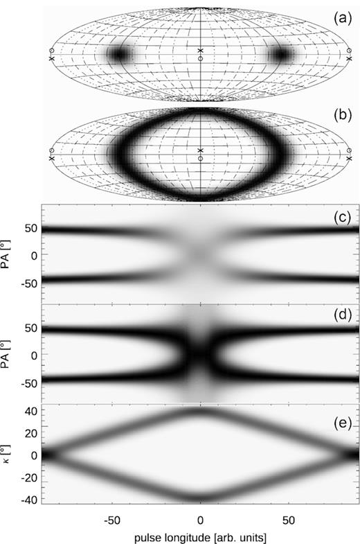
Fig. 9 shows the case of two initially orthogonal patches rotating about two different axes slightly inclined with respect to the equatorial plane (η = ±7^○). Both patches are passing on the same side of each V pole, i.e. both pass through the half-meridian zero near the poles, and none through the half-meridian of 180^○. The patches are initially located at the azimuth ±90^○ in the equatorial plane (Fig. 9a) and are subsequently being rotated by 180^○ around their axes as marked with arrows in panel (a). The left patch rotates about the axis that is cutting the P. sphere at points marked with ‘o’ signs in panels (a) and (b). The right patch rotates about the axis crossing the ‘x’ points. The upward motion of the left patch, and the downward motion of the right patch leave the round trace shown in Fig. 9(b). Tied by their near-orthogonality, the patches move in opposite directions near the V poles such that one patch crosses half-meridians with increasing values of azimuth, while the other crosses the same half-meridians in the direction of decreasing azimuth. Hence, the OPM transition takes on the ‘X’ form visible in Figs 9(c) and (d). The numerical result is consistent with the analytical solution of equation (9) (solid lines). A clearer view of the same numerical result (without the analytical solution overplotted) is reproduced in Fig. A1.

Figure 9.

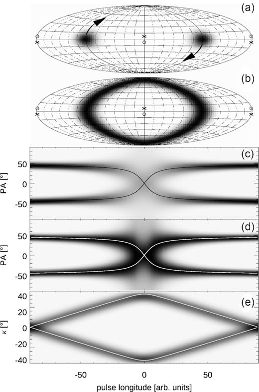
An X-type OPM transition for two patches of equal strength that pass near the V pole (η = ±7^○). (a) Initially orthogonal location of modal patches on P. sphere (Gaussian patches with 1σ width of 10^○, located at azimuths ±90^○, Hammer equal area projection). The patches are rotated around two different axes that pierce the sphere at the ‘o’ marks (left patch) or ‘x’ marks (right patch). (b) Trace of the patches after their uniform rotation by 180^○. (c) The corresponding view of the OPM transition on the standard longitude–PA diagram. Solid lines show the analytical model of equation (9). (d) Same as (c), but the greyscale is normalized for each longitude separately (black = maximum value, white = zero). (e) The corresponding ellipticity angle. White lines follow equation (8). The quantity represented by the greyscale may be considered as the histogram of the frequency of occurrence or cumulative flux.

Open in new tabDownload slide

As described in D20, the immersion of V pole within the flux patch spreads the flux across all PAs; hence, the ‘X’ structure in panel (c) becomes weak (the power is spread vertically in the longitude–PA plot). The same ‘X’ feature is shown in (d), albeit with the greyscale normalization performed for each longitude separately; i.e. the black colour in (d) corresponds to the maximum at a given longitude. This highlights the X feature.

The X form of the OPM transition resembles that observed at longitude 172^○ in PSR B1451−68 (between intervals A and B in Fig. 1). The bottom panel (e) in Fig. 9 shows the ellipticity angle that corresponds to the left half of the bow tie in Fig. 1. The numerical result follows the analytical solution of equation (8) (white lines).

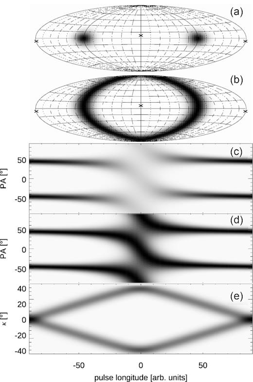
In Fig. 10, both patches are always orthogonal since they are rotated about the same axis that cuts the P. sphere at the ‘x’ marks (η = 7^○). Therefore, they pass the V poles on different sides (compare the near-polar trace of upper and lower patch motion in panel b). However, since they also traverse the azimuth in opposite directions (rightward for upper patch and leftward for lower patch) the PA curve is bending in the same direction (downwards) in each PA track (see panels c and d). This type of the OPM transition has the S-shaped form, similar to the well-known S swing of PA as caused by the unrelated RVM effect. As in the case of the X feature, each S swing in Fig. 10(c) (and 10d) is described by equation (9). As before, the ellipticity angle of Fig. 10(e) follows equation (8). A version of Fig. 10 without the analytical lines overplotted is shown Fig. A2.

Figure 10.

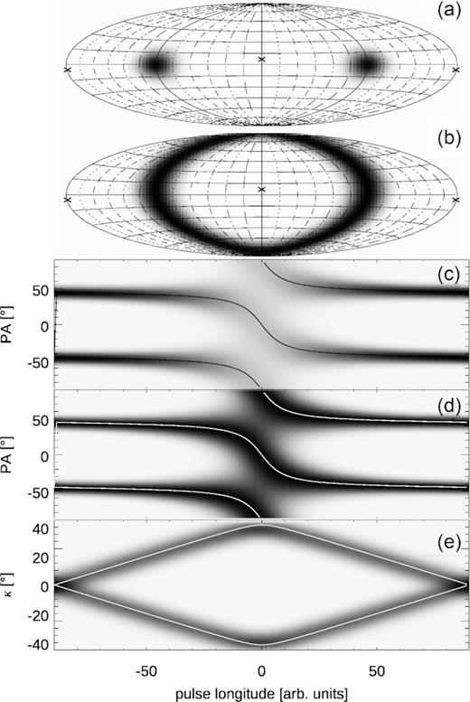
Same as in Fig. 9 except now both patches rotate around the same rotation axis with η = 7^○ (‘x’ marks). Therefore, the patches are passing on the opposite sides of the V poles. This leads to the double S-shaped OPM transition (panels c and d).

Open in new tabDownload slide

Finally, Fig. 11 shows the case where both patches stay perfectly orthogonal and pass through their V poles centrally. The patches are initially located at azimuths ±90^○ (Fig. 11a) and move purely meridionally. In the course of this rotation, each PA track spreads equally strongly up and down, forming a vertical column of weak radiative power, which looks like a break in each PA track.⁷ This type of OPM transition seems to roughly correspond to the pulse longitude of 182^○ in Fig. 1 (between intervals B and C).

Figure 11.

Same as in Fig. 10 but for η = 0; i.e. the patches move along a meridian of Poincaré sphere and pass through the V poles centrally. This leads to a pale break in the PA curve (panel c) or a dark vertical column (d).

Open in new tabDownload slide

In addition to these basic types of OPM transition, mixed cases are possible, e.g. with one PA track following the S curve while the other one follows the break as expected for central pole passage.

5.2 Patches of unequal strength

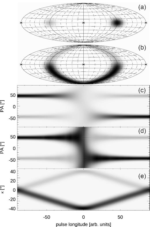
Figs 12 and 13 present the pole-passage-induced OPM transition in the case of unequal modal power. Both modal patches are Gaussians of 1σ width equal to 10^○, but the peak flux in the secondary mode patch (initially left) is at 20 per cent of the other (initially right) patch.

Figure 12.

Same as in Fig. 9 but with the initially left patch five times weaker than the right-hand side patch. The patches move around two different axes with η = ±7^○, so they pass on the same side of the V axis (as in the case of an OPM of the X type).

Open in new tabDownload slide

Figure 13.

Same as in Fig. 11 but with a five times weaker initially left patch. In this figure η = 0, which corresponds to the central VPP.

Open in new tabDownload slide

Fig. 12 shows the X-type OPM transition that is similar to the case of Fig. 9, except that two ‘arms’ of the X feature are essentially invisible (panel c) because of the weakness of the secondary mode and the vertical spread of flux across all PA values. Fig. 13 presents the case of central pole passage with the same modal power ratio (20 per cent).

6 GEOMETRIC MODEL FOR THE OPM POWER RATIO INVERSION BETWEEN THE LEADING AND TRAILING PROFILE SIDES

The polarization observed in the central part of profile (section B) in PSR B1451−68 closely resembles the expected polarization of the vacuum CR. As illustrated in Michel (1991), the CR beam is nearly fully circular in the wings, whereas it is linear in the plane of the curved particle trajectory. Indeed, the low degree of circular polarization in the centre of the profile (Φ = 178^○) is not because individual samples of opposite sign of V are averaged out, as the green curve in panel (b) of Fig. 1 demonstrates. Accordingly, while passing through the CR beam, an observer will record the polarization state that moves from one V pole to the opposite V pole (the sides of the CR beam have V of opposite handedness). This would correspond to one tilted bar (e.g.: /) in the central X-shaped part of the observed bow tie.⁸ If the middle of the vacuum CR beam is ignored, however, then the fully circularly polarized wings correspond to two opposite polarization states (+V and −V on the Poincaré sphere).

In one empirical model of pulsar polarization (D19), the two linear orthogonal modes (opposite patches on the Poincaré sphere) are formed by incidence of a circular signal on a linearly polarizing filter (as in a quarter-wave plate). To produce two different linear OPMs with uncorrelated amplitude, it was necessary to employ two circular signals of opposite handedness. The signal needed in such model is then provided by the wings of the vacuum CR beam.

Let us then assume that the emitted radio beam consists of two equally strong orthogonal modes that have their emission directions separated by a small angle relative to the electron trajectory plane. In the fan beam model of pulsar emission, the quasi-instantaneous sky-projected emission of such radiation could produce the pattern shown in Fig. 14. The strings of circles present radiation from two narrow streams of plasma flowing along magnetic field lines. The streams emerge from the vicinity of the dipole axis (near top of figure) and their projection on the sky is shown with the thick dotted lines. Emission of each stream involves two opposite polarization modes, illustrated with the grey and white circles. Their transverse separation (across the stream) reflects the finite angular size of emission beam. Local emissivity increases with the circle’s size; thus, the intensity first increases with the distance θ_m from the dipole axis, and then falls off. Because of this intensity gradient and the oblique cut through the streams, the line of sight is usually sampling unequal amounts of two OPMs (compare the size of the grey and white circles cut by the bottom path of the line of sight). However, since the tilt of the streams is opposite on the leading and trailing sides, different modes dominate in the leading and trailing sides of the profile. The ratio of OPMs depends on the angular scale of the emissivity gradient and the obliqueness of the cut. Likely effects of averaging caused by the spatial extent of the emitter are ignored here for simplicity. However, it should be noted that a uniform ring (cone) would not produce any modal imbalance – the effect is present only in the fan beam model [in the conal model, the emissivity would have to be azimuthally non-uniform (on average) for the mode imbalance to appear in average profiles]. The magnitude of mode imbalance thus depends on how non-uniform the emissivity is both in the magnetic azimuth (measured around the magnetic dipole axis) and in the magnetic colatitude.

Figure 14.

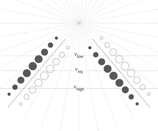
Cartoon picture of sky-projected pulsar radio emission. Strings of circles present near-instantaneous emission beams from charges streaming away from the dipole axis (central point of the radial pattern of dots near the figure top). The circles’ diameter reflects the strength of emission, whereas different colours correspond to different OPMs. Horizontal lines are paths of the sightline corresponding to different observation frequencies (the paths are different to mimic the ν-dependent size of the beam). Both OPMs are comparable in brightness at ν_eq.

Open in new tabDownload slide

Because of the spatial convolution effects, it may be impossible to directly resolve the bifurcated bimodal emission beam of Fig. 14. Even in the presence of a convolution, however, such a beam can produce the observed OPM exchange, i.e. the dominance of different OPMs in different sides of profiles (leading versus trailing). If the emissivity is strongly non-uniform in magnetic azimuth, the mode dominance can change several times within the profile (which is observed, e.g. in J0437−4715; Oslowski et al. 2014).

Note that the scenario of Fig. 14 refers to the OPM ratio inversion observed both in the patches and in the PA tracks, i.e. between the leading and trailing edges of the profile. The COMT-related VPP requires additional OPM transitions in which the flow of radiative power occurs between the orthogonal PA tracks, but not between the patches. These two types of OPM transitions coexist in the profile and they contribute to the complexity of PA tracks on the longitude PA diagrams (see D20).

6.1 Frequency dependence of real OPM power exchange

Intrinsic emission of two modes with similar strength is unlikely, because of their different amplification in anisotropic coherent processes (Melrose 2003). The model of Fig. 14 provides a geometric interpretation for a small imbalance of the modal strength in radio pulsar signal, under the assumption that equal amount of each mode is emitted in different parts of the radio beam. Comparable power in different OPMs is often observed, and sometimes one mode dominates at low ν whereas the other dominates at high ν (Young & Rankin 2012; Noutsos et al. 2015). In such case, there exists a frequency ν_eq at which both modes are perfectly equal. Strong evolution of PA tracks is observed near this transition frequency (Navarro et al. 1997; Mitra, Rankin & Arjunwadkar 2016).

These phenomena can be understood with the model of Fig. 14, assuming that the beam projections follow radius to frequency mapping; i.e. they move away from the dipole axis at low ν. Instead of three different beam positions, three different paths of sightline are marked on the same beam in Fig. 14 (solid horizontal lines). At high ν, the line of sight is traversing through the beam periphery (bottom horizontal line), so the ‘white mode’ is stronger on the leading side, whereas the ‘grey mode’ is stronger on the trailing side (compare the size of white and grey circles). At low ν (top horizontal), the grey mode is brighter on the leading side (and the white on the trailing one). At the moderate frequency of ν_eq, equal amounts of modes are observed (though not necessarily in all profile components at the same ν_eq). Since the radiation beam becomes narrower at higher ν, the spatial convolution could depolarize the profile at higher frequencies, at least in the regions with an oblique cut through the streams.

Fig. 14 implies that the ratio of OPMs is changing with Φ and ν. However, the figure predicts an essentially fixed profile width. The observed low-ν profile widening (Wu et al. 1998) must be related to the effect that causes the below-discussed interference phenomenon.

7 IMPLICATIONS FOR PHYSICS: DIRECT BEAM OR COHERENT SUPERPOSITION OF ADJACENT COMPONENTS?

7.1 Direct CR microbeam

The central part of the bow tie (section B in Fig. 1) is very similar to the polarization observed while crossing the vacuum CR beam: The polarization state travels from one V pole to the other (opposite) V pole. For example, a possible sequence of three polarization states is: +V, +Q, and −V (with all the unspecified Stokes components equal to zero). This is equivalent to the motion along half a meridian of the P. sphere. However, the polarization state observed within the full pulse window of PSR B1451−68 traces almost a full meridional circle. So the previous sequence would be extended to: −Q, +V, +Q, −V, and −Q. Thus, the polarization becomes linear in the profile wings. It is not clear whether this extra rotation of the polarization state (towards the equator of P. sphere) in the profile wings is intrinsic or results from spatial convolution or propagation effects. Definitely, the unmodified vacuum CR microbeam is not consistent with the polarization observed in PSR B1451−68.

7.2 Coherent superposition of adjacent components

The three regions of high linear polarization (A, B, and C in Fig. 1) may correspond to the three distinct profile components observed at lower frequencies (171 and 271 MHz; Wu et al. 1998). Dips (depressions) in total intensity I on both sides of the core component (at Φ = 170^○ and 184^○ in Fig. 1a) are also consistent with the triple profile form. Assuming that the adjacent components have orthogonal linear polarization (see Fig. 3b), the coherent superposition of radiation within the regions where they overlap could produce the meridional circularization. The tips of the bow tie (at κ ≈ ±45^○) would then correspond to longitudes where intensities of the modes in adjacent components are equal (to get the pure circular polarization). This interpretation is consistent with the coincidence of dips in the profile with the bow tie tips (at κ = ±45^○). Such scenario, however, employs a longitude-dependent mode brightness ratio and requires that radiation in the adjacent components maintains a fixed phase lag difference of δ = 90^○ (or at least that δ ≈ 90^○ when the components contribute equally). More specifically, the radiation in a given polarization mode in component A must be coherently summed with orthogonal mode in component B, which must be oscillating at a phase lag δ = 90^○ (as measured with respect to the oscillation in component A). Moreover, for the polarization state to continue its circulation in the same direction, the next profile component (in region C) should keep a phase lag of 180^○ with respect to component A. Thus, to keep the unidirectional rotation of the patch, the linearly polarized radiation in components A, B, and C should have the oscillation phase increasing in steps of 90^○ (e.g. 0, 90^○, and 180^○ for components A, B, and C, respectively). It is then concluded that the monotonic increase of the oscillation phase lag with pulse longitude is needed in the model based on the variable mode ratio (as determined by shapes and locations of overlapping profile components). Apparently, the components are formed by radiation with well-defined oscillation phase, which increases monotonously.

8 THE MODEL: INTERFERENCE PATTERN OF FOUR MODES

8.1 Pulsar radiation as the coherent superposition of four modes

Importantly, both the radiation in the central component (‘core’) and radiation in the ‘conal’ components consist of two polarization modes. Therefore, in the longitude intervals where the core and cone components overlap, four radiative contributions are superposed: the O and X mode of the core, and the conal O and X modes.⁹ When the O mode is coherently superposed with the X mode, the strong circular polarization appears. However, the coherent summation of the two O modes (from core and cone) only affects the intensity of the total O mode (and similarly for the two X modes). Depending on the value of the phase lag δ_oo between O_core and O_cone, the total intensity will be enhanced or reduced. The phase lag will likely depend on frequency ν and pulse longitude Φ.

If, at some frequency ν₁, the value of δ_oo(ν₁) (between O_core and O_cone, both oscillating in the same plane) is a multiplicity of 360^○, the total intensity will be stronger (positive interference). If the phase lag δ_ox between the total O mode and the remaining X mode is close to ∼90^○, their coherent superposition will produce the observed rotations of the polarization state at both sides of the core (circularization). If δ_ox ∼ 0, the PA of total signal will have the PA deflected by 45^○ away from the O and X modes (a 45^○ jump; D19). However, if there is a distribution of phase lags δ_ox between the (total) O and X modes, the observed signal will become weakly polarized (instead of circularly polarized). On the other hand, if, at some different frequency ν₂, δ_oo(ν₂) ∼ 180^○, then the two O waves will cancel each other (negative interference). This will decrease I and will produce the deep minima between the components. The flux at such minima will be dominated by the other mode (X). This must be the reason for the ubiquitous enhancement of polarization degree at minima in many pulsar profiles, e.g. in B1929+10 (Rankin & Rathnasree 1997) and in the central parts of several D-type profiles (as defined in Rankin 1983). This four-mode model thus resolves the long-standing issue of why the ‘superposition of two overlapping components’ does not depolarize the minimum between the ‘components’: The minima appear because one mode is suppressed; hence, the polarized fraction increases.

In such way, both the circularization and the minima between the components are produced by the same effect: the coherent (or partially coherent to incoherent) summation of orthogonal and parallel modes in radiation from two superposed signals (e.g. a direct beam and a reflected beam, somewhat similar to lasers, though here each beam contains two polarizations). It is then concluded that the well-separated components in the triple-form low-ν profile of B1451−68 may well have essentially the same origin as the circularization: It is the coherent summation of oscillations that are either orthogonal or parallel to each other (in various possible combinations).

8.2 The other way round: components from superposition, not superposition of components

It has been found above that different components in the average profile of B1451−68 consist of radiation with a well-defined oscillation phase (or phase lag), contrary to the mixture of phase lags that is normally expected in astrophysical sources. This macroscopic (profile-wide) structure of phase lags, along with the clearly demonstrated superposition of four modes, strongly suggest that pulsar profiles are mostly (or at least partially) an interference pattern: They must involve two radiative signals, each consisting of two orthogonal modes. The shape of profile (hence modulation properties) results from positive or negative interference of these two signals.

This means that the minima between ‘components’ in pulsar profiles are just regions of negative interference (δ_oo or δ_xx being roughly 180^○), so the ‘components’ (at least some of them) do not actually exist as separate entities – they just present the points in space–time where the interference pattern has maxima sampled by the line of sight (as determined by the usual special-relativistic detectability conditions). In other words, the observed pulsar signals represent a cut through the interference pattern, whereas the spatial emissivity distribution (i.e. shape of emission region) contributes to the profile shape, but it is not the only factor.

The model based on an interference pattern has a major advantage over a model that is plasma-density governed. Given the approximate mirror symmetry of the average profile and the axial symmetry of the open field line region, a time-symmetric refraction index and phase lag seem most natural. In the case of interference pattern, the longitude (or time) dependence of the phase lag does not have to be symmetric about the profile centre. The polarization state and its associated phase lag are determined by the space–time structure of the interference pattern.

The physical cause of this interference, which occurs within the radio pulsar beam, remains to be established. Possible processes that lead to interference include reflection (or scattering), refraction (Edwards, Stappers & van Leeuwen 2003), and emission from two sources, e.g. emission directed in opposite directions along field lines. It is also possible that the four modes originate from the linearly polarizing filtering of circularly polarized signals (D19) or elliptically polarized signals, as provided by the CR beam (Fig. 14). The conditional equivalence of two elliptical modes to the four-wave model is discussed below.¹⁰

By applying the four-mode model for PSR B1451−68, the profile can even be understood as a superposition of two triangular profiles that peak at the same longitude (Fig. 15). The deep minima observed on both sides of the central peak (‘core’) at low ν result from the negative interference, as determined by the longitude dependence of the oscillation phase (phase lag). The longitude structure of the oscillation phase, on the other hand, is intrinsic to the interference pattern. The frequency-dependent position of minima, e.g. their increasing distance at low ν, must be attributed in such model to the wavelength dependence of the interference pattern.

Figure 15.

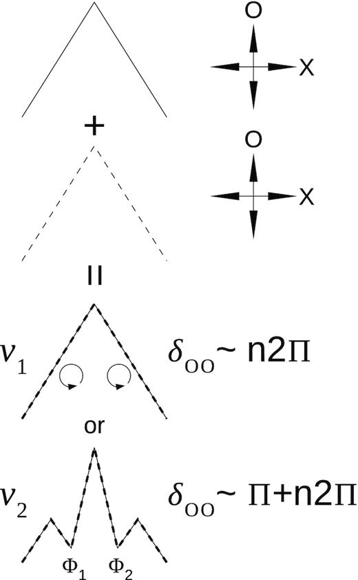
Mechanism of profile shaping by coherent superposition of two triangular profiles shown in top part of figure. Each triangle contains two orthogonal modes shown on the right. Depending on the frequency-dependent phase lag δ_oo between the two coplanar O modes, the total profile may reveal the minima (and triple form) or not. For positive interference at ν₁, the additional contribution of X mode can produce the circularization (if δ_ox ∼ 90^○). At ν₂, the two O modes cancel each other, so the presence of the X mode increases the polarization fraction at the minima (not shown). The values of δ_oo only refer to longitudes Φ₁ and Φ₂, and interference of the two X modes is ignored for simplicity.

Open in new tabDownload slide

The average profiles are known to be averaged modulation patterns. Such superposition model should thus be extended to observed time modulation effects such as drifting subpulses. An outstanding example of this phenomenon is the structure of 13 subpulses observed in PSR B0826−34 (Esamdin et al. 2005). According to the four-mode interference model, the subpulses of B0826−34 mostly originate from the phase lag structure of the superposed beams, and not from the beam pattern alone (as in the carousel model). The similar widths and separations of subpulses in such scenario thus correspond to distances in the interference pattern.

Related phenomena are the changes of modulation or subpulse drift pattern (and the associated profile modes); see e.g. fig. 1 in Weltevrede (2006). These can be interpreted as disturbances, destruction, or destabilization of the interference pattern. The interference of radiative signals is a different process than the oscillations within the emission region itself, as considered by Clemens & Rosen (2004). In particular, only the superposition of precisely orthogonal modes has been considered in Clemens & Rosen (2008) with no coplanar interference possible. In the present model, the anticorrelation between OPMs is produced through the interference of radio waves within the pulsar radio beam.

It is concluded that the so far mostly ignored necessity to take into account the coherent effects of phase lags is the key reason for several long-standing difficulties with the carousel model (Maan 2019; McSweeney 2019; McSweeney et al. 2019). The negative interference of radiative contributions oscillating in the same plane creates the illusion of components considered as separate entities. Instead, it seems there is no rotating carousel there at all – rather a different emission region with the outflowing interference pattern and the geometry of sightline sampling.

8.3 Four linear modes versus two elliptic modes

To explain the similar strength of OPMs, it has been assumed in D19 that the initial signal is circularly polarized, and it is passing through a magnetospheric region that transmits only two orthogonal linear modes (linearly birefringent filter). To finally obtain the observed two elliptical OPMs of opposite handedness, however, two circular signals of opposite handedness were needed, each one producing a pair of linear OPMs (see fig. 7 therein).

It is then concluded that the model that employs four arbitrary but linearly orthogonal waves is not equivalent to the model based on the sum of two elliptically orthogonal waves (modes). They become the same only if the two pairs of waves combine to two elliptically orthogonal waves, as represented by two antipodal states on the P. sphere. In such case, the interference does not occur (despite the coherent superposition). This is the reason why the interference term is present in equation (23) but it is missing in equation (27).¹²

The intensity-affecting interference can thus occur between imprecisely orthogonal elliptical modes. The elliptical modes in equations (23)–(26) differ in κ, so the modes are deflected from orthogonality in the meridional plane on the P. sphere. Interestingly, there are observations in which the modes are misaligned approximately in this way (e.g. B0031−07; fig. 5 in Ilie et al. 2020).

9 CONCLUSIONS

The polarization properties of PSR B1451−68 reveal that the radiative power contained within orthogonal PA tracks can change because of two independent processes: either by the near-meridional VPP of the polarization state or by the traditional change of the modal strength ratio. This reemphasizes the need to follow the variations of pulsar polarization as a function of pulse longitude on the Poincaré sphere, where the modes (patches) can be more easily separated than on the standard longitude–PA diagrams.

The meridional circularization is caused by the COMTs at the fixed quarter-wave lag (δ_ox = 90^○ + n180^○). It is not caused by the retardation (increasing δ_ox) at a fixed and equal mode amplitude. The coherent orthogonal mode transition is described by an equation of similar form to the RVM equation. Since the polarization state simultaneously takes part in two motions (RVM and VPP), the PA as a function of pulse longitude follows a curve that is the sum (equation 10) of two curves: the RVM curve (equation 11) and the RVM-like COMT curve (equation 9).

The COMT may therefore be mistaken for an RVM swing. In the quarter-wave case, the high circular polarization degree may help us to discern between these two scenarios; however, in average profiles V may be suppressed by the non-coherent contribution of the other orthogonal mode. In such case, it is useful to plot the typical instantaneous polarized fractions instead of their Stokes-based average. This COMT can also be recognized on the P. sphere. In the case of a half-wave COMT (δ_ox ∼ n180^○), the polarized fractions are not affected and the pol. state moves within the QU equator so the PA changes gradually and may be impossible to discern from RVM.

We have shown that the profile components of PSR B1451−68 consist of radiation with different and well-defined oscillation phase. The phase increases monotonously with pulse longitude and each component consists of two OPMs. Such properties imply that pulsar radio emission can be understood as the superposition of two radiative contributions, each of which contains both linearly polarized modes; i.e. the observed characteristics result from summation of four radiative contributions. This is mathematically equivalent to the superposition of two non-orthogonal elliptically polarized waves. Therefore, the profile components (hence subpulses) are determined (or at least affected) by the space–time structure (hence longitude dependence) of the phase lag between the coherently added parallel and orthogonal polarizations. To a large degree, then, the carousel (and conal) picture of the pulsar emission region may be an illusion produced by the cancelling or enhancement of coherently superposed signals.

ACKNOWLEDGEMENTS

We thank S. Johnston for help with the observations. This work was supported by the grant 2017/25/B/ST9/00385 of the National Science Centre, Poland. Pulsar research at Jodrell Bank Centre for Astrophysics and Jodrell Bank Observatory is supported by a consolidated grant from the UK Science and Technology Facilities Council (STFC). The Parkes telescope is part of the Australia Telescope National Facility that is funded by the Commonwealth of Australia for operation as a National Facility managed by CSIRO (Commonwealth Scientific and Industrial Research Organisation).

DATA AVAILABILITY

The data underlying this article can be accessed from the CSIRO Data Access Portal (https://data.csiro.au/dap), in the ATNF pulsar observation domain. The analysed data set for PSR J1456-6843 has the unique identifier t160417₋201032.sf. The data used in the calibration process have the identifier t160417₋200715.sf. The derived data generated in this research will be shared on reasonable request to the corresponding author.

Footnotes

REFERENCES

APPENDIX A

The lines described by equations (9) and (8) make the view of the greyscale patterns in Figs 9 and 10 less clear. Therefore, the figures are reproduced here without these lines. Otherwise, Figs A1 and A2 are identical to Figs 9 and 10, respectively.

Figure A1.

Reproduction of Fig. 9 without the analytical solutions of equations (9) and (8).

Open in new tabDownload slide

Figure A2.

Reproduction of Fig. 10 without the analytical solutions of equations (9) and (8).

Open in new tabDownload slide