


ABSTRACT
Massive galaxy clusters undergo strong evolution from z ∼ 1.6 to z ∼ 0.5, with overdense environments at high-z characterized by abundant dust-obscured star formation and stellar mass growth which rapidly give way to widespread quenching. Data spanning the near- to far-infrared (IR) can directly trace this transformation; however, such studies have largely been limited to the massive galaxy end of cluster populations. In this work, we present ‘total light’ stacking techniques spanning |$3.4\!-\!500\, \mu$|m aimed at revealing the total cluster emission, including low-mass members and potential intracluster dust. We detail our procedures for WISE, Spitzer, and Herschel imaging, including corrections to recover the total stacked emission in the case of high fractions of detected galaxies. We apply our techniques to 232 well-studied log|$\, M_{200}/\mathrm{M}_{\odot }\sim 13.8$| clusters in multiple redshift bins, recovering extended cluster emission at all wavelengths. We measure the averaged IR radial profiles and spectral energy distributions (SEDs), quantifying the total stellar and dust content. The near-IR profiles are well described by an NFW model with a high (c ∼ 7) concentration. Dust emission is similarly concentrated, albeit suppressed at |$r\lesssim 0.3\,$|Mpc. The measured SEDs lack warm dust, consistent with the colder SEDs of low-mass galaxies. We derive total stellar masses consistent with the theoretical Mhalo−M⋆ relation and specific star formation rates that evolve strongly with redshift, echoing that of log|$\, M_{\star }/\mathrm{M}_{\odot }\gtrsim 10$| cluster galaxies. Separating out the massive population reveals the majority of cluster far-IR emission (|$\sim 70\!-\!80{{\ \rm per\ cent}}$|) is provided by the low-mass constituents, which differs from field galaxies. This effect may be a combination of mass-dependent quenching and excess dust in low-mass cluster galaxies.
1 INTRODUCTION
Local environment plays a fundamental role in shaping galaxy properties, an effect that can be studied in its extremes in massive galaxy clusters. In the high-density cluster environments in the nearby Universe, galaxy properties differ from those of their counterparts in the field: clusters host more massive galaxies (Kauffmann et al. 2004; Collins et al. 2009; van der Burg et al. 2013), with a strong preference for lower star formation rates (SFRs; Balogh et al. 1998; Lewis et al. 2002; Peng et al. 2010) and early type morphologies (i.e. Dressler 1980). These differences, well established by a wealth of detailed studies in the local and low redshift Universe, have prompted the often challenging task of pushing into the high-redshift cluster and proto-cluster regimes. This is necessary in order to construct an evolutionary picture of environmental effects on galaxy populations, which ties into the broader question of large-scale structure formation.
Optical and near-infrared (IR) observations of clusters beyond the local Universe have found that cluster populations have colours, luminosity functions, and stellar ages consistent with a model of very early (z ≫ 2–3), vigorous stellar mass growth followed by largely passive evolution (i.e. Stanford, Eisenhardt & Dickinson 1998; Blakeslee et al. 2006; van Dokkum & van der Marel 2007; Eisenhardt et al. 2008; Mei et al. 2009; Mancone et al. 2010). Mid- and far-IR studies have shown this picture to be incomplete, however, with many intermediate redshift (z ∼ 1–2) massive clusters hosting heavily obscured star forming galaxies (SFGs), indicating a deviation from the local SFR–density relation at this epoch (i.e. Cooper et al. 2006; Hilton et al. 2010; Tran et al. 2010; Fassbender et al. 2011, 2014; Hayashi et al. 2011; Tadaki et al. 2011; Brodwin et al. 2013; Zeimann et al. 2013; Alberts et al. 2014; Bayliss et al. 2014; Santos et al. 2014, 2015; Ma et al. 2015; Alberts et al. 2016). Deep Spitzer Space Telescope and Herschel Space Observatory 1 observations of rich z ∼ 1–2 clusters find (dust-obscured) galaxies with SFRs and specific SFRs (SSFRs) comparable to the field down into the cluster cores at z ≳ 1.4 (Brodwin et al. 2013; Alberts et al. 2014, 2016) followed by rapid evolution that establishes the largely quenched cluster populations at z ≲ 1 (Muzzin et al. 2008). Combined with studies of coeval quenched cluster populations (i.e. Nantais et al. 2017; Chan et al. 2019), it has emerged that z ∼ 1–2 is a transitional era for rich, massive clusters from abundant (obscured) star formation and active galactic nuclei (AGN) activity (Martini et al. 2013; Alberts et al. 2016) to widespread quenching.
The importance of obscured activity at intermediate redshifts extends organically into the proto-cluster regime, where there is increasing evidence that overdensities of dusty SFGs (DSFGs; Casey, Narayanan & Cooray 2014) are often the signposts of proto-cluster candidates (Casey 2016). These early, potentially coeval DSFGs (Umehata et al. 2015, 2017; Casey 2016; Clements et al. 2016; Kato et al. 2016; Arrigoni Battaia et al. 2018; Greenslade et al. 2018; Lewis et al. 2018; Oteo et al. 2018; Cheng et al. 2019; Harikane et al. 2019; Lacaille et al. 2019) are natural candidates for the precursors to the massive end of later cluster populations, particularly massive ellipticals (i.e. Hopkins et al. 2008).
Taken together, these high-redshift cluster and proto-cluster studies indicate that infrared-emitting dust is clearly an important tool for studying the evolution of (proto-)clusters. However, IR studies – and cluster galaxy studies in general – have been mostly confined to looking at individual members at the bright, massive end of the cluster populations. A full accounting of the dust emission in (proto-)clusters requires a different approach to constrain the faint contributors: low-mass cluster members and potential emission from intracluster dust (ICD; Dwek, Rephaeli & Mather 1990) embedded in the hot intracluster medium. Statistical methods that average multiple clusters through stacking (Dole et al. 2006) have been used on local and low-redshift samples to characterize total cluster properties and place upper limits on the IR emission from ICD (Kelly & Rieke 1990; Montier & Giard 2005; Giard et al. 2008). Recently, this technique has been expanded to the proto-cluster regime: Planck Collaboration XXVII (2015) obtained targeted Herschel/SPIRE follow-up and stacked 220 cluster candidates at 2 ≲ z ≲ 4 from the Planck Catalogue of Compact Sources (PCCS; Planck Collaboration XXIX 2014), finding a strong detection of extended far-IR emission on the spatial scales associated with proto-clusters (Chiang, Overzier & Gebhardt 2013). Kubo et al. (2019) stacked 179 proto-cluster candidates at z ∼ 3.8 selected from the Hyper Suprime–Cam Subaru Strategic Program (HSC–SSP; Aihara et al. 2018) at multiple wavelengths, including imaging from the Wide-Field Infrared Survey Explorer (WISE), Herschel, and Planck. This study revealed intense star-forming environments with warm stacked spectral energy distributions (SEDs) suggestive of AGN activity.
The Planck Collaboration XXVII (2015) and Kubo et al. (2019) results demonstrate the power of statistical stacking analyses for studying total cluster IR emission up to the high-redshift, proto-cluster regime. In this work, we develop multiwavelength stacking procedures to probe the ‘total light’ in clusters and proto-clusters for wide-field data sets such as the all-sky WISE and wide-area Herschel SPIRE surveys. Here, ‘total light’ refers to the (background subtracted) summation of all light in a sample of clusters without the identification of individual constituents. Stacking near-IR to far-IR data sets allows us to probe both the existing stellar content and ongoing mass growth over a range of redshifts and halo masses, constraining the dust content, SEDs, and mass assembly from low-redshift clusters to clusters at cosmic noon to proto-clusters at z ≳ 2. In this work, we test our techniques on a well-studied massive cluster sample at z ∼ 0.5−1.6 in the Boötes field (Eisenhardt et al. 2008), taking advantage of ancillary data and providing the first analysis of the total stellar content and dust emission in massive clusters into the era of active star formation at z ∼ 1–2.
Section 2 describes our cluster sample and the data sets used in this work. In Section 3, we describe our stacking techniques, including image pre-processing and photometry. We additionally discuss the applicability of our technique to other (proto-)cluster samples, presenting a correction factor for data sets that lack cluster member information. Section 4 tests our stacking technique on clusters in the Boötes field, analysing the average radial profiles and total photometry in multiple redshift bins. We further build ‘total light’ SEDs and compare the total output to the output from massive cluster members only. Section 5 discusses our results and Section 6 presents our conclusions. Throughout this work, we assume a WMAP9 cosmology (ΩM, ΩΛ, h) = (0.28, 0.72, 0.70) (Hinshaw et al. 2013) and a Chabrier (2003) IMF.
2 DATA
2.1 Cluster sample
The IRAC Shallow Cluster Survey (ISCS; Eisenhardt et al. 2008) contains over 300 galaxy cluster candidates from 0.1 < z < 2, with >100 at z > 1, in the Böotes field (α, δ = 14:32:05.7,+34:16:47.5). Cluster identification was performed using a wavelet search algorithm to find galaxy overdensities in the rest-frame near-IR in 3D space (RA, Dec., photometric redshift) using flux-limited 4.5 |$\, \mu$|m imaging from the IRAC Shallow Survey (Eisenhardt et al. 2004) and full photometric redshift probability distribution functions derived from combined deep optical BWRI from the NOAO Deep Wide-Field survey (NDWFS; Jannuzi & Dey 1999) and IRAC 3.6 and 4.5|$\, \mu$|m imaging (Brodwin et al. 2006). Due to the flux-limited nature of the IRAC Shallow Survey (8.8|$\, \mu$|Jy, 5σ, at 4.5|$\, \mu$|m; Eisenhardt et al. 2004), this cluster catalogue is approximately stellar mass selected. Cluster centres are adopted from the centroid of the wavelet detection algorithm and thus trace the distribution of massive galaxies.
Spectroscopic follow-up of ISCS cluster candidates, shown in Fig. 1, by the AGN and Galaxy Evolution Survey (Kochanek et al. 2012) has confirmed dozens of clusters at z < 1. At z > 1, over 20 of the ISCS clusters have been spectroscopically confirmed through targeted follow-up with the Low-Resolution Imaging Spectrometer on Keck (Oke et al. 1995) or Hubble Space Telescope Wide Field Camera 3 (Kimble et al. 2008) spectroscopy (see Stanford et al. 2005; Brodwin et al. 2006, 2011; Elston et al. 2006; Eisenhardt et al. 2008; Zeimann et al. 2012; Brodwin et al. 2013; Zeimann et al. 2013). The photometric redshift accuracy for the confirmed ISCS clusters is |$\sigma = 0.036\, (1+z)$|; no cluster candidates were confirmed at a substantially different redshift than predicted, though we note that the targeted spectroscopic follow-up was limited to the most robust cluster candidates. Among the cluster candidates not spectroscopically confirmed, we expect the ISCS to have a |$\sim 10{{\ \rm per\ cent}}$| false detection rate due to chance line-of-sight projections (Eisenhardt et al. 2008).
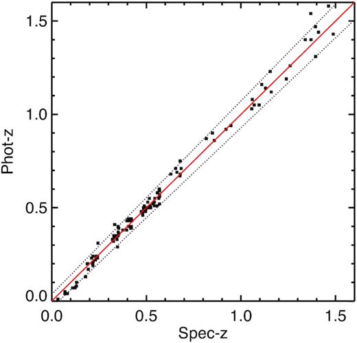
Comparison of the photometric redshifts for clusters in the ISCS sample with spectroscopic confirmation from the MMT (Kochanek et al. 2012), Keck (Stanford et al. 2005; Brodwin et al. 2006; Elston et al. 2006; Eisenhardt et al. 2008), and HST (Brodwin et al. 2011; Zeimann et al. 2013). The dotted lines show the scatter in cluster photometric redshift accuracy, |$\sigma = 0.036\, (1+z)$|.
ISCS cluster halo masses (quantified throughout as M200, the mass interior to R200, the radius at which the mean mass density exceeds 200 times the critical density) have been determined through a combination of targeted follow-up of confirmed clusters and statistical arguments. X-ray observations (Brodwin et al. 2011, 2016) and weak lensing (Jee et al. 2011) have found that high-richness z > 1 ISCS clusters have halo masses in the range log M200/M⊙ = 14−14.7, with the full ISCS sample having typical halo masses of log M200/M⊙ = 13.8−13.9, determined using clustering measurements (Brodwin et al. 2007) and halo mass ranking simulations (Lin et al. 2013; Alberts et al. 2014). From these works, it was also determined that there is no significant redshift evolution in the median halo mass of ISCS clusters. This means that due to the selection technique, this cluster sample is not a progenitor sample, but rather provides snapshots of clusters at an approximately fixed halo mass at different epochs. ISCS clusters at z ∼ 0.5 (z ∼ 1.5) have expected halo masses of |$\sim \!1\times 10^{14}\, \mathrm{M}_{\odot }$| (|$\sim \!3\times 10^{14}\, \mathrm{M}_{\odot }$|) at z = 0, with a factor of 2 scatter (Chiang et al. 2013).
In this work, we utilize 232 ISCS clusters from 0.5 < z < 1.6 (Table 1) to perform a ‘total light’ cluster stacking analysis. These redshift bounds are chosen to avoid the steep angular size-redshift relation at z < 0.5 and small number statistics in the cluster sample at z > 1.6 due to increasing photometric redshift uncertainties. Given the typical ISCS halo mass, the median virial radius of our cluster sample is |$R_{200}\approx 1\,$|Mpc (Brodwin et al. 2007), which we adopt throughout this study.
Sample Statistics.
| Sample | Redshift | # | zmean | zmedian | Avg. |$\#$| of photo-z |
|---|---|---|---|---|---|
| members per clustera | |||||
| ISCS | 0.5 < z ≤ 0.7 | 61 | 0.57 | 0.55 | 30 |
| (Boötes) | 0.7 < z ≤ 1.0 | 78 | 0.86 | 0.87 | 33 |
| 1.0 < z ≤ 1.3 | 53 | 1.13 | 1.15 | 24 | |
| 1.3 < z ≤ 1.6 | 40 | 1.44 | 1.45 | 11 |
aFor cluster members within 1 Mpc with log |$M_{\star}$|/M⊙ ≥ 10.1
Cluster membership was determined for these clusters via spectroscopic redshifts, where available, and full photometric redshift probability distribution functions as described in Eisenhardt et al. (2008), Brodwin et al. (2013), and Alberts et al. (2014). The photometric redshift catalogue used in this work was presented in Alberts et al. (2016), following the procedure in Chung et al. (2014), which incorporates near-IR observations from the Infrared Boötes Survey.2 Stellar mass estimates for individual galaxies were calculated using optical-mid-IR SEDs for all sources in the Spitzer Deep Wide-Field Survey (SDWFS; Ashby et al. 2009), as described in Brodwin et al. (2013).
In Fig. 2, we show representative IR data centred on a galaxy cluster at z = 1.09. Photometric redshift cluster member positions are marked therein.
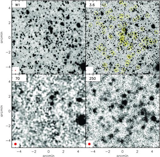
A 10 arcmin × 10 arcmin image centred around ISCS J1425.6+3403, a galaxy cluster at z = 1.09, is shown in the WISE W1 (top left), IRAC 3.6|$\, \mu$|m (top right), MIPS 70 |$\, \mu$|m (bottom left), and SPIRE 250 |$\, \mu$|m band (bottom right), respectively. Image point spread function FWHM is indicated by a red circle at bottom left corner of each panel. All photometric redshift member candidates are marked as the yellow circles in the 3.6 |$\, \mu$|m image, together with 1 and 2.5 Mpc radius circles around the cluster centre. Varying imaging depths and angular resolutions are apparent, highlighting the challenges in studying the properties of individual cluster galaxies except for the most luminous ones.
2.2 Herschel imaging
Herschel SPIRE (Griffin et al. 2010) coverage of the Böotes field was obtained as part of the Herschel Multi-tiered Extragalactic Survey (HerMES; Oliver et al. 2012). The Herschel SPIRE 250, 350, and 500 |$\, \mu$|m imaging was done in a two-tiered design centred on (α, δ) = (14:32:06,+34:16:48) with a deep survey covering the inner two square degrees, and a shallower survey covering 8 deg2. The data reduction, presented in Alberts et al. (2014), was done using the Herschel Interactive Processing Environment (HIPE v7; Ott 2010) with a particular emphasis on the removal of striping through high-order polynomial baseline removal and the removal of glitches. The pipeline-reduced SPIRE maps have a zero mean and are calibrated to units of Jy beam−1. Full width at half-maximum (FWHM), pixel scale, and 5σ depth for the three SPIRE bands are listed in Table 2. The 1σ confusion limits for 250, 350, and 500|$\, \mu$|m are 5.8, 6.2, and 6.8 mJy, respectively (Nguyen et al. 2010). Data reduction, catalogue creation, and completeness simulations of the Böotes SPIRE maps used in this work are described in Alberts et al. (2014).
Key characteristics of data used in this work.
| Band name | Effective wavelength | Filter widtha | FWHM | Pixel scale | 5σ | Reference |
|---|---|---|---|---|---|---|
| (μm) | (μm) | (arcsec) | (arcsec pix−1) | (μJy) | ||
| unWISE W1 | 3.35 | 0.73 | 6.1 | 2.75 | 54 | Lang (2014), Meisner et al. (2017a), Meisner et al. (2017b) |
| unWISE W2 | 4.60 | 1.10 | 6.4 | 2.75 | 71 | – |
| IRAC 3.6 |$\, \mu$|m | 3.55 | 0.75 | 1.66 | 0.863 | 2.91 | Ashby et al. (2009) |
| IRAC 4.5 |$\, \mu$|m | 4.49 | 1.02 | 1.72 | 0.863 | 4.61 | – |
| IRAC 5.8 |$\, \mu$|m | 5.73 | 1.43 | 1.88 | 0.863 | 25.35 | – |
| IRAC 8.0 |$\, \mu$|m | 7.87 | 2.91 | 1.98 | 0.863 | 28.84 | – |
| Band name | Effective wavelength | Filter width | FWHM | Pixel scale | 5σ | Reference |
| (μm) | (μm) | (arcsec) | (arcsec/pix) | (mJy) | ||
| WISE W3 | 11.56 | 8.30 | 6.5 | 1.375 | 0.7 | Wright et al. (2010), Cutri et al. (2013) |
| WISE W4 | 22.08 | 3.50 | 12.0 | 1.375 | 5.0 | – |
| MIPS 24 |$\, \mu$|m | 23.68 | 4.7 | 6.0 | 1.245 | 0.2 | Jannuzi et al. (2010) |
| MIPS 70 |$\, \mu$|m | 71.42 | 19.0 | 18.0 | 4.925 | 31 | – |
| SPIRE 250 |$\, \mu$|m | 243 | 78 | 18.1 | 6 | 14–26 | Oliver et al. (2012) |
| SPIRE 350 |$\, \mu$|m | 341 | 106 | 24.9 | 10 | 11–22 | – |
| SPIRE 500 |$\, \mu$|m | 482 | 200 | 36.6 | 14 | 14–26 | – |
aFor the WISE filters, filter widths are approximately measured as full width at half-maxima of the total response function, which includes quantum efficiency, transmission of optics, beamsplitters, and filters. The IRAC sensitivities refer to those measured in 3 arcsec-diameter circular apertures (Ashby et al. 2009).
2.3 WISE imaging
The WISE mission covered the full sky with four bands centred on 3.4|$\, \mu$|m (W1), 4.6|$\, \mu$|m (W2), 12|$\, \mu$|m (W3), and 22|$\, \mu$|m (W4). The raw images have a field of view 47 arcmin × 47 arcmin that is imaged simultaneously via dichroics on the four detectors at a pixel scale of 2|${_{.}^{\prime\prime}}$|75 pix−1. The full description of the mission is provided in Wright et al. (2010). The ‘ALLWISE’ data combined the data taken as part of the four-band cryogenic survey (2010 January 7–August 6), 3-Band Cryo phase3 (W1, W2, and W3 only with the W3 band at reduced sensitivity; 2010 August 6–September 29), and the first year data from the ‘Near Earth Object Wide-field Infrared Survey Explorer (NEOWISE) post-cryo’ program (September 29, 2010 – February 1, 2011 with W1 and W2 only; Mainzer et al. 2011). The NEOWISE reactivation (NEOWISE-R) program, which began in 2013 October, and continues to this day, have thus far produced six separate data releases.
The ALLWISE data release4 (Cutri et al. 2013) includes ‘Atlas Images’, each tile of which covers |$1.56\deg \times 1.56\deg$| in area. These images are resampled to 1|${_{.}^{\prime\prime}}$|375 pix−1, i.e. a half of the native pixel scale, and convolved with the instrument point spread function (PSF). While these smoothing steps help detect isolated point sources from the final coadded images, the procedure (and the resultant blurring) is less desirable while photometering fainter individual sources near the detection threshold.
In this work, we use a new set of coadds of the WISE images referred to as the unWISE 5 data set. While the details of the image processing steps are described in Lang (2014) and Meisner, Lang & Schlegel (2017a), one of the main differences lies in that it preserves the instrument PSF and the native pixel scale with no additional blurring. We use the unWISE ‘NEOWISE-R3’ images (Meisner, Lang & Schlegel 2017b) for the W1 and W2 bands, which combine the first 4 yr of WISE observations (including 3 yr of the NEOWISE operations). In particular, we use the ‘masked’ coadds in which outlier pixels are rejected in the image combination.
For the W3 and W4 bands, we use the official AllWISE Atlas images. This is mainly because the unWISE products for these bands are known to contain artefacts around bright sources (Lang 2014); this is in contrast to the W1/W2 products that were further improved by adding depth and removing artefacts as more post-cryogenic data were added for processing (Meisner et al. 2017b). We note that ALLWISE and unWISE data should yield identical results for stacking analyses given everything else equal. Indeed, we have verified that this is the case for the original (cryogenic) mission data (Wright et al. 2010; Lang 2014).
The PSF widths are ≈6 arcsec for the unWISE W1 and W2 bands, i.e. smaller than 8 arcsec for the same band in the ALLWISE data (Wright et al. 2010; Meisner & Finkbeiner 2014). As mentioned previously, this difference stems from additional convolution performed by the latter. The ALLWISE and unWISE images share the same pointing centre. The ALLWISE tiles are 4095 × 4095 at the pixel scale 1|${_{.}^{\prime\prime}}$|375 pix−1 while the unWISE tiles are 2048 × 2048 at the scale 2|${_{.}^{\prime\prime}}$|75 pix−1. Adjacent tiles overlap approximately 4 arcmin in both data sets.
A total of 11 tiles (tile numbers: 2156p348, 2170p318, 2177p333, 2192p348, 2201p363, 2159p333, 2174p348, 2182p363, 2163p363, 2188p318, and 2195p333) cover all of our clusters. The median number of individual exposures is in the range 130–155 in the W1 and W2 bands, and 21–32 in the W3 and W4 bands. Given that exposure time per visit was 7.7 s (W1 and W2) and 8.8 s (W3 and W4), the total exposure time per pixel is 16.7–19.9 min and 3.1–4.7 min, respectively. For further information on WISE depths and pixel scales, see Table 2.
2.4 Spitzer/IRAC and Spitzer/MIPS imaging
For Spitzer IRAC imaging, we use the final data release of the SDWFS catalogue, which provides deep IRAC imaging over the entire NDWFS field proper from which our clusters are selected. The observations and processing of the data are given in Ashby et al. (2009). The 5σ limiting flux densities within 3 arcsec aperture diameters are 2.91, 4.61, 25.35, 28.84 μJy at 3.6, 4.5, 5.8, and 8.0 |$\, \mu$|m. We use the MIPS data taken for the MIPS AGN and Galaxy Extragalactic Survey (MAGES; Jannuzi et al. 2010), reduced using the MIPS–GTO pipeline (Gordon et al. 2005), with 5σ point source sensitivities of 0.2 and 31 mJy at 24 and 70 |$\, \mu$|m. All Spitzer data are single mosaicked images in units of mJy sr−1. The pixel scale is 0.86 arcsec for the IRAC bands, 1.245 arcsec for the MIPS 24|$\, \mu$|m band, and 4.925 arcsec for the 70 |$\, \mu$|m band (see Table 2 for a summary).
3 ‘TOTAL LIGHT’ CLUSTER STACKING METHOD
In this section, we present our ‘total light’ stacking techniques for WISE, Spitzer, and Herschel imaging. To reiterate, ‘total light’ is the summed light from all cluster constituents, including previously unidentified (mostly low mass) cluster members and/or ICD components. We note that our Herschel stacking technique is similar to those previously presented in the literature (i.e. Béthermin et al. 2010; Planck Collaboration XXVII 2015); however, WISE and Spitzer stacking are more complicated due to the much higher source density (of cluster members and non-members both) and non-uniform sky background. We explore several methods for WISE/Spitzer cluster stacking and conclude this section with a discussion on which methods are appropriate given the available data.
Total light cluster stacking was recently used to analyse proto-cluster candidates in Planck Collaboration XXVII (2015) and Kubo et al. (2019). In Planck Collaboration (2015), proto-cluster candidates selected as cold, compact Planck sources (Planck Collaboration XXIX 2014) were used as positional priors to stack Herschel SPIRE imaging. The technique used, presented in Béthermin et al. (2010), averages SPIRE cut-outs centred on the Planck sources, after cleaning the cut-outs of bright sources, to obtain the pixel-WISE average flux and create a final stacked image.
Kubo et al. (2019) performed multiwavelength stacking on WISE, IRAS, AKARI, Herschel, and Planck images of proto-cluster candidates from the HSC–SSP. For reference, we summarize their stacking technique for the data sets (WISE and Herschel) relevant to this work: sky-subtracted images were obtained using sky maps generated by evaluating the local (in scales of ≈10 arcmin) sky values after masking bright sources. Stacking was then performed on the sky-subtracted images as an average stack with 3σ clipping, with uncertainties measured via bootstrapping. For WISE stacking, Kubo et al. (2019) smoothed the sky-subtracted images to the Planck PSF (≈5 arcmin) prior to stacking; for Herschel, they carried out stacking on both the original and smoothed maps.
3.1 Image stacking
3.1.1 WISE/Spitzer Image Processing
The varying angular resolution and image depth of our data sets pose a significant challenge in measuring the total IR flux from clusters. In WISE and Spitzer data, the number of both cluster and non-cluster galaxies detected individually in the image varies significantly across the passbands. The overall source density is much greater at shorter wavelength (e.g. W1, W2, 3.6, 4.5 μm bands) at which low-redshift galaxies (low-level star formers and passive galaxies) are intrinsically brighter. Hence, a single bright foreground source can bias the flux measurement along cluster sightlines. To minimize these effects, we process WISE and Spitzer images following a procedure modified from that described in Xue et al. (2017). Their procedure was used to measure extended low surface brightness (SB) Ly α emission from distant star-forming galaxies. We provide a full description of the adopted procedure below.
First, we remove all individually detected sources from each image. This is done by running the sextractor software (Bertin & Arnouts 1996) on each science image which outputs a source catalogue, sky background map, and segmentation maps. Typically, we use a DETECT_THRESH of 3.0 and a DETECT_MINAREA of 3, requiring the isophotal signal-to-noise ratio to be 5 or higher. Secondly, we use the sextractor-generated sky background map to perform an additional pass of sky subtraction. The images we use already have their sky background close to zero; the median sky estimated using the iterative sigma-clipping algorithm is 10–20 per cent of the pixel-wise rms. However, large-scale variations of the sky background are present – due to instrument defects and bright sources – which can adversely impact the stacking procedure. To avoid eliminating the cluster signal as background, we set the sextractor BACK_SIZE to be no less than 10 arcmin in all cases. At the cluster redshift range, 10 arcmin corresponds to 4–5 Mpc, much larger than the angular extent of the emission.
Finally, we use the source segmentation map and create several different versions of the science images. In the first image, which we will refer to as a ‘_masked’ image, we mask sources detected by sextractor as indicated by the segmentation map by replacing their pixels with NaN. In the second ‘_unmasked’ image, we unmask the pixels belonging to the photometric-redshift-selected (photo-z) cluster members (Section 2.1), and repeat the same procedure. Doing so ensures that all fluxes from the photo-z cluster members are preserved in the image. Other sources remain masked. Cluster members that are identified via spectroscopic redshifts only are not included in order to maintain a uniform stellar mass cut. The third ‘_sub’ image is simply a sky-subtracted image where all sources (cluster and non-cluster) are present. In all three versions, the values of unsegmented pixels are identical throughout the image.
The procedure of masking and unmasking described above is performed separately on each band. While applying the same set of masks uniformly in all bands may result in a cleaner and more consistent measurement of cluster light, it is neither practical nor feasible to cleanly mask/unmask the cluster members from these images as they increasingly blend with other sources and occupy a significant fraction of the cluster region in the sky at longer wavelength (see Fig. 2). In Section 3.2, we discuss how this masking/unmasking process can impact our measurements.
For the WISE data, the same procedure is repeated after we create a large mosaic by combining the tile images. Doing so ensures the full extent of the data are utilized properly for cluster members that lie close to the edge of a WISE tile. Further, this streamlines the procedure as the Spitzer data are already in a single mosaic format. We reproject each WISE tile using a common tangent point (the centre of the tile 2174p348), and run the iraf task mscred.mscstack to combine them (offset = world, combine = average). Reprojection of the WISE tiles at a new tangent point leads to non-integer shifts of the images. That combined with the overlap between adjacent tiles (≈4 arcmin or ∼80–90 image pixels) results in lower sky rms values in the mosaicked image in these regions, which is entirely artificial. To circumvent this problem, we expand the projected bad pixel masks to minimize the image overlap.
3.1.2 WISE/Spitzer image stacking
For each cluster, we create a 28 arcmin × 28 arcmin image for each wavelength centred on its position using the IDL routine hastrom.pro. Counts are converted to physical units (μJy pix−1) at this stage. For the WISE data, we use the photometric zero-points given in the image header.6 For the IRAC and MIPS data, we simply multiply the image by an appropriate scale factor to convert from mJy sr−1 to μJy pix−1. For a given sample consisting of N clusters, the procedure creates a 3D datacube. Image stacking is then performed by collapsing the datacube along the first dimension by taking pixel-wise mean or median.
As described in the previous section, three different image stacks are created using the ‘_masked’, ‘_unmasked’, and ‘_sub’ images. For the _masked and _unmasked datacubes, the flagged (NaN) pixels are excluded from the considerations. We repeat this stacking procedure for non-cluster sightlines. For each of the N clusters, we pick a random position 12–24 arcmin from the cluster centre. In Fig. A1, we illustrate the stacked WISE W2 images of the cluster and non-cluster sightlines using four different images, namely, mean_unmasked, mean_masked, median_masked, and median_sub.
Towards the cluster sightlines, we detect extended emission spanning ≈2 arcmin across (0.7–1.0 Mpc at z = 0.5−1.6). While the ‘off-cluster’ image stack is clearly devoid of any emission at the centre, it exhibits similar noise properties to the cluster stacks, which is reassuring. In Table A1 and Fig. A1, it is also evident that the noise properties vary depending on the precise stacking method. The sky noise does not obey a pure Poisson statistic in any of the stacks, and the mean_unmasked stack shows the highest root mean square in sky pixels. The correlated non-Poisson noise is likely brought on by the angular distribution of faint sources not flagged by the above procedure. This is consistent with the expectation that the mean pixel combination should be more susceptible to their presence than the median combination. A full description of our results using different image versions and comparisons is given in Appendix A. The interpretation of these different stacking schemes is discussed in Section 3.2.
3.1.3 WISE/Spitzer photometry
On the image stack, we determine the centroid of the stacked signal using the IDL routine gcntrd.pro. The offset of the centroid from the image centre is small – typically less than 2–3 arcsec. Such an offset has a negligible effect on the flux measurements although it can affect the shape of the radial profile near the peak.
To measure the total flux from our cluster stack, we perform aperture photometry. First, we estimate sky in annular bins in the range of 150–200 arcsec. This is necessary particularly for the _unmasked stack in which cluster member candidates are unmasked. Because they are identified out to 2.5 Mpc from cluster centre (Eisenhardt et al. 2008), doing so artificially increases the source density out to the same distance. Indeed, this effect is clearly visible in several short-wavelength bands where a large fraction of cluster member candidates are individually detected. We stress that the effect is entirely artificial. The median image stack, which does not include the fluxes of individual sources, does not show the same level of rise in the baseline at the same angular range, though some bands do show a much lower level of the same effect, suggesting that galaxies falling in towards the clusters that lie much farther than 2 Mpc may play a minor role. Setting the baseline at larger radii would increase the flux up to 30 per cent.
In all WISE and Spitzer bands, we measure the cumulative fluxes in a series of circular apertures with a stepsize of 5.5 arcsec, i.e. twice the native WISE pixel scale. The cumulative fluxes are simply a sum of all pixel values (post-sky subtraction) within the given aperture. The radial SB is measured as the mean of all pixels in annuli with the same stepsize.
We examine the intensity distribution of sky pixels, and find that it is skewed towards the high-end wing. This is expected given that some pixels must contain fluxes of unresolved faint sources even after sky subtraction. The ‘straight-up’ standard deviation of the distribution is larger by up to a factor of ≈2 than a sigma-clipped value, σp, i.e. a Gaussian fit to the pixel distribution. However, the result is insensitive to a specific choice of a sky annulus. The level of deviation from a pure Gaussian depends on the underlying flux distribution of all sources and what we define as a ‘source’ (i.e. the specific setting of our source detection with the sextractor software such as DETECT_THRESH and MINAREA). The formal errors for the mean SB and for the cumulative flux are |$\Delta S = \sigma _{\rm p}/\sqrt{N_a}$| and |$\Delta F = \sqrt{N_c}\sigma _{\rm p}$|, where Na and Nc are the number of pixels within a given annulus and aperture, respectively. However, these estimates are based on a single sky annulus and thus do not account for possible variations in σp within the stacked image.
We test the stability of measured σp values by examining the mean and rms values of the sky on annuli centred on 500 randomly chosen locations in the off-cluster stack. The relative fluctuation of the σp values in the off-cluster stack is 2–11 per cent for the Spitzer bands, and up to 1 per cent for the WISE bands. In addition, we find that the mean sky varies 1–17 per cent for the Spitzer bands and 0.5–4 per cent for the WISE bands. The largest fluctuation in both sky mean and rms values occurs in the 8.0 |$\, \mu$|m band.
Taking these measurements as different realizations of the sky for the cluster signal, we obtain a more realistic estimate of our measurement uncertainties. The total pixel-to-pixel fluctuation is calculated as |$\sigma _{\rm T}^2 = \sigma _{\rm p}^2 + \sigma _{\rm sky}^2 + \sigma _{\rm rms}^2$| where σsky and σrms are the standard deviation of sky background (i.e. mean sky) and pixel rms, respectively, determined from the 500 off-cluster stack measurements. Including these factors increases the photometric errors by a factor of ≈2–5 in the Spitzer/WISE bands.
3.1.4 Herschel/SPIRE image processing
We do not perform any additional image processing of the SPIRE maps prior to stacking. The pipeline reduced SPIRE maps have a zero mean and thus are already background subtracted. Source masking is similarly not required. Unlike Spitzer and WISE, the SPIRE imaging is confusion limited (see Section 2.2) and so the vast majority of sources, both cluster and field, are expected to be individually undetected. This was confirmed for cluster members in Alberts et al. (2014), which found that |$\lesssim 10{{\ \rm per\ cent}}$| have a candidate 5σ counterpart at 250|$\, \mu$|m. This leaves the dominant detected population: field galaxies. Since field galaxies exist across the zero mean maps, they should not contribute to the stacked signal, which we verify in the next section.
3.1.5 Herschel/SPIRE image stacking
Clusters are stacked in the three SPIRE bands by building a 3D datacube comprised of 28 arcmin × 28 arcmin (roughly 2 × Rvir at z ∼ 1) cut-outs centred on each cluster. Each cut-out is randomly rotated to avoid systematic offsets. The SPIRE stacks are then created by taking the variance-weighted mean of each pixel across all cut-outs. As discussed in Alberts et al. (2014), a variance-weighed mean is appropriate for the two-tiered Boötes SPIRE survey, which has differing depths and therefore differing noise properties across the map.
The contribution from the field galaxy population, detected or undetected, is determined by stacking cut-outs placed randomly off of any known cluster. While the stacks towards clusters display clearly detected extended emission, the stacks away from clusters show no stacked signal above the noise. This test verifies that the stacked signal from the field population is zero, as one would expect in a zero mean map. Example stacks towards and away from the cluster sightlines can be seen in Fig. C1 in Appendix C.
We determine the centroid and rough widths of the SPIRE stacks by approximating them as a Gaussian using the idl code mpfit2dpeak (Markwardt 2009). The Herschel stacks have a approximate FWHM of ∼600 kpc at all redshifts; the radial profiles will be more carefully examined in Section 4.1. Centroiding is performed on the full set of bootstrap realizations to get the best estimate of the stack centres. In our initial centroiding of the SPIRE stacks, we discovered a systematic offset of 1–2 pixels in the x,y centre of the extended cluster emission. As this offset persisted across all cluster sub-sets and simulated data (see Appendix C), we determined it was a systematic of the data, likely the scan pattern, rather than a real effect. In order to be conservative, we randomly rotate the SPIRE cut-outs centred on each cluster while stacking. This eliminates the offset and allows us to centroid on the stacked cluster centres for aperture photometry. The resulting radial profiles and aperture fluxes are identical within the uncertainties, regardless of cut-out rotation.
3.1.6 Herschel/SPIRE photometry
As with the WISE and Spitzer stacks, the Herschel stacked emission is clearly extended and so aperture photometry is performed on the stack images (after converting from Jy beam−1 to Jy pix−1) using the python package photUtils (Bradley et al. 2019).
The uncertainties on the flux in a given aperture are determined via bootstrapping with replacement, whereby the cluster catalogue is resampled and stacked at random, allowing duplicates, 10 000 times. Aperture photometry is performed on each bootstrap realization, and the mean and standard deviation of the resulting distribution represent the statistical properties of the clusters being stacked. As discussed in Alberts et al. (2014), this method captures not only detector and confusion noise, but also the relative spread in the population being stacked. The bootstrapped mean is checked for consistency with the stacked mean, which reassures us that the stacked signal is not dominated by a few outliers.
3.2 Measuring cluster light: understanding the meaning of stacked fluxes
As described in Sections 3.1.1 and 3.1.2, each Spitzer and WISE image is prepared in several different ways in which the treatment of the pixels belonging to detected sources differ. Starting from these images, four different image stacks are created (mean_unmasked, mean_masked, median_masked, and median_sub). While we present a detailed comparison of the measured fluxes and the statistical properties in Appendix A, here we consider the physical meaning of their differences in the context of cluster light.
The ISCS data set used in this work has unique advantages that are typically not shared by a vast majority of other cluster samples. First, the availability of multiple passbands of varying depths and of overlapping wavelength ranges enables us to explore the usefulness of the shallower WISE data in carrying out similar analyses in the future on other cluster samples. The agreement between WISE and Spitzer IRAC bands at similar wavelengths (e.g. W1 versus 3.6 |$\, \mu$|m and W2 versus 4.5 |$\, \mu$|m) is excellent in both measured fluxes and radial profile shapes, as detailed in Appendix B. Thus, applying similar stacking techniques to larger cluster samples using only the WISE bands should yield robust results to constrain the overall stellar content and their internal distributions.
Secondly, the ISCS cluster sample has superb photometric redshifts (in addition to extensive spectroscopic redshifts of members), information that is often limited or unavailable for other larger cluster surveys. In this work, we have taken advantage of this photo-z information and ‘unmasked’ cluster members in the image (_unmasked) where all the sources are otherwise masked. This step verifies that the stacked signal is not dominated by unfortuitously positioned non-member galaxies (or stars) that are bright.
In all the images we have tested, we consistently find that the mean_unmasked stack always yields the largest aperture fluxes; the other three stacks – namely, mean_masked, median_masked, and median_sub – show comparable fluxes to one another, which are consistently lower than the mean_unmasked stack. The agreement of these three stacks assures us that the statistical background subtraction of non-cluster galaxies is effective, and as a result, we can recover fluxes of faint cluster members. It also implies that as long as we treat all images consistently (in measuring sky background and in detecting and removing individual sources), we can expect a robust result. This may be in part owing to the fact that the present data set is relatively uniform in coverage and depth. The possibility of combining heterogeneous data sets (e.g. varying exposure time across a given field) would require further investigation.
The difference between the mean_unmasked and mean_masked stacks can only be interpreted as the unmasked cluster members positively contributing to the resultant flux in the former. The fact that the mean_masked and median_masked stacks yield similar fluxes strongly suggests that a large fraction of cluster light originates from the numerous faint members that lie below the detection threshold rather than from a few relatively bright members that eluded photo-z identification. In the latter scenario, the overall pixel distribution would be highly asymmetric resulting in its mean significantly greater than the median. Finally, it is reassuring that the median_sub stack fares well providing an estimate robust against a range of bright sources present in the images; the fact that it returns a comparable flux to the other two _masked stacks reinforces the notion that numerous undetected cluster members raises the overall counts in the cluster regions.
In this interpretation, both fluxes convey distinct physical significance. The mean_unmasked-derived fluxes represent total fluxes coming from clusters encompassing all member galaxies (and possibly from ICD) regardless of their intrinsic brightness. For the remainder of this work, we will refer to this flux as ‘total flux’ and ‘total light’ with regard to the near- and mid-IR stacks. Informed masking of the images ensures that all possible members are available for counting while sky counts on off-cluster pixels carry information on statistical background (from non-cluster-members). On the other hand, the remaining stacked fluxes with no photo-z member information represent the cluster fluxes originating from the sources that are too faint to be detected. In the case of the stacks presented in Appendix A, these faint galaxies are responsible for ≈60–70 per cent of the total cluster flux (Table A1).
The number of cluster members that rise above the detection limit depends on a number of factors: imaging depth, cluster luminosity function, distance (thus, redshift) to the cluster, and wavelength. We compute the fractional contribution to the total cluster flux from detected sources in all Spitzer and WISE bands for our four redshift samples, computed as |$f_{\rm det}\equiv 1-F_{\rm others}/F_{\rm mean\_unmasked}$| where |$F_{\rm mean\_unmasked}$| denotes the flux measured from the mean_unmasked stack while, for Fothers, we use the fluxes measured from the median_masked, mean_masked, and median_sub stacks.
In Tables 3 and 4, we list the range of fdet for the WISE and Spitzer bands, respectively. We give both the mean (of the three others stacks) as well as the typical uncertainties. At longer wavelength and at higher redshift, our estimates tend to become less certain. Whenever the uncertainties become comparable to or larger than the mean correction, we list the range of the fdet instead of the mean. Whenever the fluxes from the median stacks become larger than the fiducial mean_unmasked, we choose not to list the fdet, as it likely suggests that the signal is too noisy to place a meaningful constraint.
Fraction of total flux above the detection limit, |$f_{\rm det}\equiv 1-F_{\rm others}/F_{\rm mean\_unmasked}$| where others refers to median_masked, mean_masked, or median_sub, for WISE imaging. A circular aperture of 100 arcsec in radius is used.
| Sample | W1 | W2 | W3 | W4 |
|---|---|---|---|---|
| z = 0.5−0.7 | 68 ± 3% | 47 ± 8% | 18 ± 13% | 0–6% |
| z = 0.7−1.0 | 62 ± 4% | 32 ± 8% | 1–3% | 1–5% |
| z = 1.0−1.3 | 51 ± 6% | 32 ± 9% | 2–4% | 5–11% |
| z = 1.3−1.5 | 17–27% | 20–44% | – | – |
| Sample | W1 | W2 | W3 | W4 |
|---|---|---|---|---|
| z = 0.5−0.7 | 68 ± 3% | 47 ± 8% | 18 ± 13% | 0–6% |
| z = 0.7−1.0 | 62 ± 4% | 32 ± 8% | 1–3% | 1–5% |
| z = 1.0−1.3 | 51 ± 6% | 32 ± 9% | 2–4% | 5–11% |
| z = 1.3−1.5 | 17–27% | 20–44% | – | – |
Fraction of total flux above the detection limit, |$f_{\rm det}\equiv 1-F_{\rm others}/F_{\rm mean\_unmasked}$| where others refers to median_masked, mean_masked, or median_sub, for Spitzer imaging. A circular aperture of 100 arcsec in radius is used.
| Sample | |$3.6\, \mu$|m | |$4.5\, \mu$|m | |$5.8\, \mu$|m | |$8.0\, \mu$|m | M24 | M70 |
|---|---|---|---|---|---|---|
| z = 0.5−0.7 | 72 ± 3% | 62 ± 4% | 31 ± 17% | 28 ± 16% | 26 ± 14% | 0–20% |
| z = 0.7−1.0 | 73 ± 3% | 64 ± 5% | 27 ± 18% | 3–14% | 29 ± 8% | 0–19% |
| z = 1.0−1.3 | 60 ± 4% | 51 ± 12% | 19–37% | 18–23% | 0–20% | 34 ± 24% |
| z = 1.3−1.5 | 52 ± 22% | 42 ± 18% | 0–14% | 9–24% | 0–7% | – |
Comparing the values listed in the tables, it is evident that the Spitzer band has higher fdet than that in the WISE band at similar wavelength. This simply reflects the better sensitivity and angular resolution of the IRAC data compared to the WISE observations. It is also notable that fdet declines precipitously with increasing wavelength such that at 8 μm, no more than 10–20 per cent of the cluster light lies above the detection threshold.
Our results demonstrate the overall usefulness of the stacking approach in recovering the full extent of the emission originating from clusters. Equally importantly, we stress that it may be possible to use a careful calibration, such as that presented here, to fully utilize the power of all-sky missions such as WISE. Given that the WISE coverage is largely uniform across the whole sky, one can use the information given in Table 3 as a correction factor to go from the measured WISE flux to the total flux for data sets where cluster membership is not known. For example, for the z = 0.5−0.7 clusters, Table 3 lists fdet = 0.68 for the WISE W1 band. If one makes a measurement of the W1 band flux f for a different sample of clusters at similar redshift (using methods similar to our median_masked, or median_sub stacks), the total flux is expected to be fcorr = f/0.68 ≈ 1.47f.
We intend to investigate this further using a larger sample of clusters and across multiple cosmic epochs in the future. As the mean_unmasked stacks represent all cluster light (regardless of direct detection of the source), our main results in this work are based on those stacks unless stated otherwise.
4 RESULTS
Using the techniques outlined in Section 3, we stack the ISCS clusters in four redshift bins: 0.5 < z ≤ 0.7, 0.7 < z ≤ 1.0, 1.0 < z ≤ 1.3, and 1.3 < z ≤ 1.6 (Table 1). The size of the bins reflects the need to detect a significant stacked signal across a broad wavelength range while ensuring that the angular scale does not change substantially within a given redshift bin.
In Fig. 3, we show the 1.0 < z ≤ 1.3 cluster stacks at all wavelengths: WISE W1, W2, W3, W4, IRAC 3.6, 4.5, 5.8, and 8.0|$\, \mu$|m, MIPS 24 and 70|$\, \mu$|m, and SPIRE 250, 350, and 500|$\, \mu$|m. For the near- and mid-IR bands, we use the mean_unmasked images for stacking analyses. These panels are arranged in the order of increasing wavelength starting from top left. The stacked signal is resolved in all cases, even at 500 |$\, \mu$|m where the beamsize is 36 arcsec (∼ 300 kpc at z ∼ 1.2). In the following sections, we analyse the radial profiles of the ISCS clusters as a function of wavelength and redshift and compare to an NFW profile (Navarro, Frenk & White 1996) as the fiducial cluster profile. In addition to being commonly used to model dark matter (DM) haloes, the NFW profile can be used to describe the cluster stellar mass distribution (e.g. Lin, Mohr & Stanford 2004; Muzzin et al. 2007; van der Burg et al. 2014; Hennig et al. 2017; Lin et al. 2017). We then determine the total cluster flux at each wavelength and redshift and build ‘total light’ cluster SEDs. In the final section, we measure the stacked far-IR emission from massive galaxies (log M⋆/M⊙ ≥ 10.1) only, using the techniques from Alberts et al. (2014), to facilitate a comparison of the behaviour of massive cluster galaxies to the total far-IR emission.
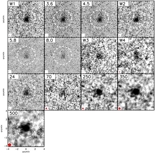
Mean (mean_unmasked) stacks of the ISCS clusters at z = 1.0−1.3 showing extended cluster emission from |$3.4-500\, \mu$|m. A higher source density within ≈4 arcmin radius is apparent in several bands including the 3.6|$\, \mu$|m, 4.5|$\, \mu$|m, and W1 bands. The effect is artificial and is brought on by an enhanced source density around clusters as discussed in Section 3.1.3. Local sky background is always estimated within this range for accurate sky subtraction. Image point spread function FWHM is indicated by a red circle at bottom left corner of each panel.
4.1 Radial flux profiles
In Fig. 4, we show the radial SB profiles measured for the z = 1.0−1.3 clusters. For the Spitzer and WISE bands, the annuli increase in steps of 5.5 arcsec, i.e. twice the native WISE pixel scale, 2.75 arcsec. For the Herschel SPIRE bands, half the FWHM for each band is used as the radial bin size (Table 2). In each panel, the profile is normalized at 27.5 arcsec to be at 0.5, a value chosen arbitrarily for vizualization. The unWISE W1 band profile is additionally overlaid as thick grey line on all panels.
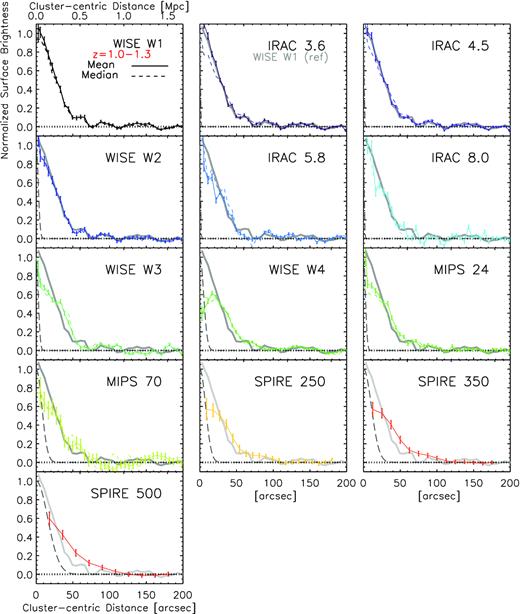
The observed radial surface brightness profiles of WISE, Spitzer, and SPIRE image stacks of the z = 1.0−1.3 clusters, arranged in the order of increasing wavelength. All profiles are normalized to have the value 0.5 at 27.5 arcsec. The long-dashed lines show the PSF size approximated as a Gaussian. In each panel for W1 through MIPS 70 |$\, \mu$|m, we show the measurements from both the mean (solid) and median (dashed) stacks. The two profiles are typically consistent with one another except at the inner ≈30 arcsec. The grey solid line in each panel marks the radial profile (mean_unmasked) of the W1 band as a reference.
The overall agreement between the measured profiles in the WISE and IRAC bands at similar wavelengths is remarkably good considering the range of imaging depth and angular resolution spanned by these data. Similar agreements exist in the other redshift bins. At longer wavelengths, the profiles tend to become shallower than the reference (W1 band: the grey line); this is particularly the case for the SPIRE bands. Keeping in mind that the SPIRE bands have considerably larger beam FWHMs as well as pixel scales, a more careful analysis to account for these differences is needed to evaluate the overall similarities of profiles at near- and far-IR wavelengths, which we discuss in Section 4.1.2.
The profiles measured from the mean_unmasked and median_unmasked stacks (the solid and dashed line, respectively, in each of the WISE and Spitzer panels) are in good agreement with each other except for the inner ≈30 arcsec. The physical explanation may be that the overall distribution of faint cluster galaxies is similar to that of their brighter cousins while there is an excess of brighter galaxies at the cluster core pulling up the mean (see our discussion in Section 3.2). Among those bright galaxies that affect the core profile are the brightest cluster galaxies (BCGs). We do not take the extra step of removing the BCGs from our radial profiles, however, as previous studies have found that their impact on the stellar mass profiles is small (van der Burg et al. 2015). Regardless of the origin, the agreement is promising for constraining the cluster light profiles based on larger cluster samples for which photometric redshift information is unavailable (discussed in Section 5.6.3).
If the angular extent measured from our image stacks carries physically meaningful information, our stacking approach could potentially provide a powerful tool in tracing past and current star formation activity within clusters encoded at rest-frame near-IR and far-IR wavelengths, respectively. Applying this technique to all-sky surveys will prove particularly promising. To further investigate this possibility, we assess the usefulness of such measurements by comparing our radial profile measurements with those obtained by a more conventional method where more detailed information is available, albeit for fewer clusters.
4.1.1 The effects of beamsize and centroid uncertainties
In order to compare our radial profiles to a fidicual profile, we need to address observational effects. For example, Fig. 4 shows that the profiles are becoming shallower at longer wavelengths. This effect is most obvious in the MIPS 70|$\, \mu$|m band and Herschel bands. The decreasing S/N and increasing pixel scales and beamsizes are expected to effectively broaden the profile relative to the intrinsic one.
Here, we address several observational factors that affect our radial profile measurement. First, unlike cluster studies largely based on spectroscopic members, our determination of cluster centres is only accurate within 15 arcsec. The precision of the ISCS cluster centroids derives largely from the 15 arcsec pixel scale of the density maps used for cluster detection. A detailed analysis in the similarly selected MaDCoWS cluster sample, which used density maps with the same resolution, confirmed rms scatters of ≈15 arcsec in both right ascension and declination (Gonzalez et al. 2019). Comparison of the ISCS centroids with the X-ray centroids for a small number of high-redshift clusters finds consistent offsets (Garcia et al., in preparation).
Secondly, a PSF at a given wavelength will systematically move the flux in the inner part outwards, the degree of which depends on the beam size and pixel sampling. Both factors effectively blur the intrinsic profile, resulting in a shallower radial profile than the intrinsic one.
Once these effects are quantified, we can infer the intrinsic profile by making the appropriate correction. We start by creating a simulated cluster whose radial profile follows a projected NFW profile. Since we are only interested in the relative change in SB, our models have a single parameter, i.e. profile scale length rs, which is related to the concentration parameter (c ≡ R200/rs). At a fixed rs value and fixed redshift, we create an image positioned at image centre, representing the true profile. Then, we create 100 images of the same profile but with a random offset drawn from a normal distribution with a standard deviation of 15 arcsec. A mean stack of these images is created, resampled, and convolved appropriately to match those of a given band. We approximate the IRAC PSFs to be a Gaussian with the pre-warm-mission full-width-at-half-maximum values7 given in the IRAC Instrument Handbook. For the WISE bands, we use the WISE instrument PSF (Wright et al. 2010; Meisner & Finkbeiner 2014) to represent the unWISE data at the native pixel scale. The Herschel SPIRE PSFs are modeled as 2D Gaussians with the appropriate FWHM (Table 2).
Radial profiles of the simulated images are measured in the same manner as real data (Section 4.1). In Fig. 5, we illustrate how the intrinsic SB of three NFW profiles (rs = 0.05, 0.10, and 1.0 Mpc at z = 1.2, panel a) is altered by the uncertainty in cluster centroid determination (panel b) plus pixel sampling and instrument beamsize (PSF; panel c). The relative change – quantified by the ratio of observed to intrinsic at a given angular scale, i.e. (c)/(a) – depends on the steepness of the intrinsic profile, which is illustrated in panel (d). In all but panel (d), all profiles are normalized at the smallest radial bin for clarity. It is evident that the observed profile of the more concentrated NFW model (rs = 0.1 Mpc) shows a more pronounced depression near the centre while showing an excess at 20–40 arcsec. While the centroid errors, pixel scale, and beamsize always play a role, the factor dominating the correction needed to recover the intrinsic profile depends on the observation parameters. As expected, the centroid errors are the most important factor in correcting the Spitzer and WISE bands, while the beam and pixel size dominate for the SPIRE bands (see Table 2). Finally, we note that the correction factor also has a mild dependence on redshift due to the change in angular scale.

The effects of centroiding uncertainties, pixel sizes, and beam (PSF) sizes are illustrated assuming source redshift z = 1.2. In all but (d) panels, all surface brightness profiles are normalized to match at the smallest radial bin for clarity. (a) The intrinsic profile with the scale lengths rs = 0.05 (dashed), 0.10 (solid), and 1.00 Mpc (dot–dashed). (b) The profiles shown in panel (a) are randomly offset from the true centre assuming a Gaussian distribution with σ = 15 arcsec. 100 different realizations are then averaged to create an ‘observed’ profile. (c) The average profile in panel (b) is convolved with the PSF of the IRAC 3.6 |$\, \mu$|m (top) and with the SPIRE 250 |$\, \mu$|m beamsize (bottom) as indicated by the grey long-dashed lines. (d) the correction factor to recover the true profile can be estimated by taking the ratio of the intrinsic and mock observed profiles (panel a and c, respectively) at a fixed scale. The thick red lines mark unity.
In Fig. 6, we demonstrate how the observed and intrinsic (corrected) profiles compare in the 3.6 |$\, \mu$|m band using our measurements for the z = 1.0−1.3 sample. For this, we have assumed 20 NFW profiles with the scale lengths between 0.02 and 1.0 Mpc. The virial radius R200 at this redshift is ≈1 Mpc (Brodwin et al. 2007), and thus, these profiles have concentration parameters c (≡ R200/rs) in the range 1–50. All curves are normalized such that at rnorm = 0.35 Mpc (≈40 arcsec at z = 1.15), they match the measured SB given in units of μJy pix−1. This normalization radius is chosen such that the cluster-centric distance is not too close to the range where the correction required for the SB profile is significant (≲30 arcsec: see the right-hand panel of Fig. 5), but also is not too far such that the signal is still robust.
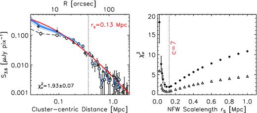
Our determination of the best NFW model is illustrated. We simulate 20 NFW profiles with scale lengths ranging rs = 0.02−1.0 Mpc, for each of which 20 Monte Carlo realizations are created to account for centroiding errors and beamsize. Left: the uncorrected mean surface brightness profile from the mean_unmasked stacks (white circles) in the 3.6 |$\, \mu$|m band is shown for the 1.0 < z ≤ 1.3 clusters. Corrections are then applied based on these models to restore its intrinsic profile (the blue lines). The corrected profile is then compared to the underlying profile (the red line) to obtain the goodness-of-fit |$\chi _\nu ^2$|. Mean and standard deviation of 20 different realizations are indicated on bottom left corner. We also show van der Burg et al. (2014) measurements for cluster galaxies at z ∼ 1 (the grey triangles), which are in good agreement with our corrected profile realizations (the blue lines). All profiles are normalized at rnorm = 0.35 Mpc as indicated by a vertical dotted line. Right: The computed reduced chi-square values for the 3.6 μm band are shown as filled circles at 20 different rs values. Highly concentrated NFW profiles in the range of rs ≈ 0.1–1.5 Mpc are strongly preferred. The W1-band measurements yield similarly low rs values (the open triangles).
We derive the correction factor for the SB profiles as follows. We assume that all 100 simulated clusters lie at the same redshift (zmean = 1.13), while their centroids offset randomly from the image centre in the angular direction. For each NFW model, we create 20 different realizations, thus there are 20 possible ways to correct the observed SB profile. As can be seen in the left-hand panel of Fig. 6, the level of uncertainties in the appropriate correction factor is at best modest and limited to r ≲ 10 arcsec. We show the observed profile as white circles (and dashed line). For clarity, each of the 20 corrected profiles are shown as a solid blue line without error bars; the underlying NFW profile is indicated as a red line. The wiggles in the observed SB (the white circles) at ≳60 arcsec are likely due to a combination of the intrinsic faintness of the cluster signal and the contributions from interlopers. The latter is clearly present in the mean stack of the 3.6 |$\, \mu$|m band shown in Fig. 3 as sources lying outside the virial radius.
We determine the best-fitting model by evaluating the goodness of fit of the corrected SB measures to the model NFW profiles. The rs = 0.13 Mpc model provides the best fit as can be seen in the measured |$\chi ^2_\nu$| values shown in the right-hand panel of Fig. 6. The normalization distance has a small impact on the goodness of fit. For example, if we normalize at rnorm = 0.3 Mpc, both rs = 0.13 and 0.15 Mpc models yield similar |$\chi ^2_{\nu }$|. However, larger rs (i.e. lower concentration parameters) models are never favoured as they have |$\Delta \chi ^2_{\nu } = 2-10$|. We confirm that the best-fitting model remains unchanged when we substitute the full, extended IRAC point response function (sampling out to 150’ from the source centre) instead of a Gaussian kernel approximating the core PSF. We repeat the fitting procedure for the W1 band by comparing the observed W1 profile with model simulations with the W1 band PSF, and obtain a similar range of rS as best-fitting models as shown in the right-hand panel of Fig. 6 (the open triangles). This is not surprising as the two profiles are nearly identical as illustrated in Fig. 4. The difference in the PSF size matters little in this case as both profiles are substantially more extended than the respective PSFs.
Finally, we test the robustness of our results against two possibilities. First, it is possible that the background level (i.e. the zero-point of the measured profiles) may be overestimated due to the fluxes of infalling galaxies at cluster outskirts. To test this, we have added a constant to each radial bin in increments of of 1 × 10⁻³ up to 5 × 10⁻³ μJy pix−1. As a reference, a typical uncertainty in the radial SB at ≈100 arcsec is ≈(2−3) × 10−3 μJy pix−1 for the 3.6 |$\, \mu$|m band. Doing so slightly alters the |$\chi ^2_\nu$| but does not change the best-fitting model, which remains in the range rs = 0.13−0.15 Mpc. Secondly, we change the redshift distribution of the clusters. Instead of assuming the mean redshift for all clusters, we populate them at random within the range z = 1.0−1.3 and scale their overall SB – according to the cosmological dimming and the change in the angular scale – before averaging them into a single profile. Once again, doing so does not change the best-fitting model.
In the 3.6 |$\, \mu$|m band, our measurements are in remarkably good agreement with those measured by van der Burg et al. (2014), which are shown as the grey triangles in Fig. 6. In that work, the stellar mass density of individually detected galaxies was measured (|$80{{\ \rm per\ cent}}$| completeness at log M⋆/M⊙ = 10.16), which should in principle scale linearly with the 3.6 |$\, \mu$|m band brightness. The agreement lends us confidence that the radial profile measurements derived from our cluster stacking analysis can yield physically useful insight into the overall distribution of light, provided that measurement biases and uncertainties are well understood and fully taken into account in the analysis.
4.1.2 The change of cluster radial profiles with wavelengths and redshift
The profile shapes at near- and far-IR wavelengths probe past and current star formation activity by sampling stars and dust-obscured star formation, respectively, assuming the contribution from ICD is negligible (see Section 5.1 for a broader discussion on this assumption). By comparing the two we may be able to examine how the cluster environment influences its member galaxies at a given cosmic epoch. Moreover, by measuring the redshift evolution of cluster radial profiles, we can trace the overall effect of its growth (via accretion of more haloes, and star formation activity). In this subsection, we investigate how measured cluster profiles change with wavelength and redshift.
In Fig. 7, we show the measured profiles in the 3.6 |$\, \mu$|m and SPIRE 250 |$\, \mu$|m bands for the four redshift subsamples, with the z = 1–1.3 bin reproduced as a reference on all panels. Overlaid are two NFW profiles (rs = 0.13 and 0.50 Mpc) convolved with the instrument PSF and centroid uncertainties (see Section 4.1.1). The similarity of the measured profiles across the full redshift range is striking. In all cases, a highly concentrated NFW model (c ≳ 7) is preferred over a much shallower model (c ≲ 3). Physically, the 3.6 |$\, \mu$|m radial profiles are straightforward to interpret: in the ISCS cluster redshift range, the IRAC 3.6 |$\, \mu$|m band samples λrest = |$1.5\!-\!2.3 \, \mu$|m, and thus is sensitive to total stellar mass content within the cluster. Taken at face value, our results suggest that the cluster stellar mass profile changes little over cosmic time. We postpone discussing this result in comparison with the literature to Section 5.5; here we focus on evaluating its robustness. Specifically, if we are systematically oversubtracting the sky from the cluster signal, the effect can mimic a steep profile. This is conceivable for the near-IR wavelengths given that we have no choice but to estimate the local sky background at ≲250 arcsec – due to the distribution of cluster members identified via photometric redshifts (Section 3.1.1) – where any NFW profile is expected to have a non-zero signal. The SPIRE stacking is not expected to be affected by local oversubtracting as the sky background is relatively uniform and subtracted on much larger scales.
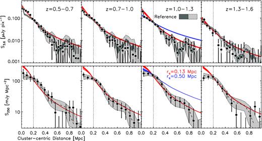
Radial SB profile measurements for the 3.6 |$\, \mu$|m (top) and SPIRE 250 |$\, \mu$|m (bottom) bands are shown for our four redshift bins. In all panels, the hatched regions represent our measurements for the z = 1.0−1.3 bin for the given band shown as a reference. For the IRAC profiles (top), we show two different ranges of uncertainties, namely, photometric errors (the fluctuations of the mean and rms of the sky, light grey errors bar for the individual profiles and shaded region for the reference) and possible variations in the mean sky across the full survey field. The two are added in quadrature (the thick error bars). Two simulated NFW profiles, corrected for our centroiding uncertainties and beamsize – rs = 0.13 Mpc (red) and 0.50 Mpc (blue) – are shown to illustrate the steepness of the profile and the range of variations affecting the profile at the smallest scale due to the centroid uncertainties. All profiles are normalized at 0.2 Mpc.
We test this possibility using the simulated NFW profiles spanning rs = 0.1–0.3 Mpc in scale length at z = 1.15. At 200–250 arcsec, the SB level falls off to 0.5–2.0 per cent of that measured at 5.5 arcsec, which is the first angular bin at which our measurements are made. The higher SB at large radius corresponds to the larger rs (smaller c) value. Scaling from the observed profiles in the same band, the expected correction should be no larger than 2 × 10⁻⁴ μJy pix−1.
In addition to the above bias, we also assess our ability to estimate the sky background, which can also artificially alter the profiles at large radii to be steeper or shallower than the intrinsic one. As described in Section 3.1.3, each individual image is processed to have ‘zero sky’ before stacking. Since the number of clusters in all four redshift bins is comparable and the IRAC coverage is uniform across the survey field, the expectation is that the residual sky in the stacked images would also be similar. We have checked this and found that the sky background – measured in the same angular annulus in all cases – can vary within (2−3) × 10−4 μJy pix−1.
In Fig. 7, we have added additional uncertainties of 4 × 10⁻⁴ μJy pix−1 (i.e. slightly larger than the quadratic sum of the two sources of error) to the error budget to illustrate how such corrections would affect the NFW profile fit. These are shown as the hatched regions for the reference sample (our z = 1–1.3 redshift bin), and the thick error bars for the data, respectively. The original errors are shown as the dark grey shades and as the light grey bars in the same figure. While local sky subtraction will have a tendency to artificially steepen the profiles, the effect is too small to significantly alter the inferred rs values. Thus, we conclude that the intrinsic profiles of cluster light must be steep.
We also examine how the profiles change with wavelength by comparing the IRAC and SPIRE measurements. In the lower panels of Fig. 7, it is clear that at small scales (r ≲ 0.3 Mpc), the SPIRE measurements fall below the best-fitting NFW model. In contrast, the IRAC data points are reasonably well described by the steep NFW profile at all scales. If the observed far- and near-IR flux trace dusty star formation activity and existing stars, respectively, the comparison of the two profiles can tell us about how the specific (dusty) SFR varies with cluster-centric distance (modulo the SPIRE beam).
In order to study this behaviour more clearly, we convolve the stacked IRAC images of each redshift sample with the SPIRE 250 |$\, \mu$|m beam approximated by a 2D Gaussian kernel with FWHM = 18.1 arcsec (Table 2). The radial profile is measured directly from the convolved image. In the top panels of Fig. 8, we show the SPIRE SB profile rescaled to match the IRAC profile at r = 0.2 Mpc. Suppression of far-IR flux relative to IRAC near the cluster core is evident in all redshift bins.
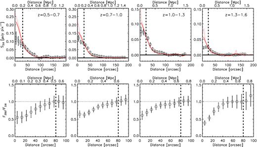
Comparison of the surface brightness and flux ratio measurements in the 3.6 and 250 |$\, \mu$|m bands. Top panels: the IRAC profiles convolved with the SPIRE 250 |$\, \mu$|m beamsize (the red solid line) are compared with the 250 |$\, \mu$|m data (the open circles). The latter is rescaled to match the IRAC measurements at r = 0.2 Mpc. The unconvolved IRAC SB is shown as a red-dotted line. The relative deficit of SPIRE flux at the cluster core is apparent. Bottom panels: the ratio of the cumulative fluxes (F250/F3.6). Both fluxes are normalized at 80 arcsec.
The absolute magnitude of the deficit – defined as ΔS3.6–250 ≡ S3.6−S250 – is the greatest in the lowest redshift bin (z = 0.5−0.7). This is not surprising because they suffer the least amount of cosmological SB dimming: i.e. given everything equal, both their luminosities and SB (at mid-IR wavelength in the observer’s frame) are higher than those of the higher redshift clusters. Additionally, lower redshift clusters may be intrinsically more luminous due to the continued mass assembly process in clusters.
An ideal measure to quantify the suppression of far-IR emission in clusters free of these effects would be ΔS3.6–250/S3.6, a fractional deficit normalized by the IRAC SB at a given radial bin. However, such a measure proves problematic. First, both ΔS3.6–250 and S3.6 asymptote to zero at large radii, making the measure very noisy. Imperfect sky subtraction can have an exacerbating effect by either exaggerating the noise or suppressing the trend. As discussed earlier in this section, the oversubtraction of the sky background in the IRAC stack almost certainly plays a role.
To circumvent these issues, we show the ratio of the cumulative fluxes, F250/F3.6, in the bottom panels of Fig. 8. Both fluxes are normalized to match at 80 arcsec. Unlike the SB ratios, the flux ratio is insensitive to where we normalize. The deficit of the SPIRE flux is still evident in all redshift bins although now it should be interpreted as the suppression of the dusty SF averaged within the given circular region, and not as a proxy for the SSFR at the given cluster-centric distance.
There is a slight hint that the region of suppressed SF is widening with cosmic time. For the clusters in the z = 0.5−0.7 bin, the flux ratio increases slowly and approaches unity at ≈0.5 Mpc. On the other hand, for the highest redshift clusters, the increase is a steeper function of cluster-centric distance, and reaches unity at ≈0.3–0.4 Mpc. The virial radii of these clusters are expected to be similar in both redshift bins (Brodwin et al. 2007). However, the trends seen in all redshift bins are comparable within the uncertainties.
All in all, we find strong evidence for the suppression of dusty star formation activity in cluster cores in all probed redshift ranges. In order to better quantify the redshift evolution (in both magnitudes and physical scales of the SF suppression), larger cluster samples are needed, which will improve the precision with which we can measure the profile shapes and the sky background.
4.2 Total cluster flux and spectral energy distributions
In this section, we combine our full stacking results and radial profile analysis in order to measure the total cluster flux as a function of wavelength and redshift. The total fluxes are then used to build the total cluster light SED. Fig. 9 shows the cluster stacks in all redshift bins for a representative set of observed wavelengths: 4.5|$\, \mu$|m probes the stellar content of the clusters, 8 and 24|$\, \mu$|m probe the warm dust content and polycyclic aromatic hydrocarbon (PAH) features, and 250 |$\, \mu$|m traces the far-IR cold dust emission reprocessed from star formation (plus any ICD component, if present).
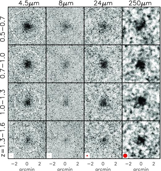
Image stacks in the IRAC 4.5 |$\, \mu$|m, 8 |$\, \mu$|m, MIPS 24 |$\, \mu$|m, and SPIRE 250 |$\, \mu$|m bands are shown for four redshift bins. The brightening at far-infrared wavelength relative to the near-infrared with increasing redshift is apparent, perhaps indicating larger dust content and higher star formation activity at larger look-back time. In the first column, we also show a circular aperture corresponding to 1 Mpc in radius (the white-dashed circles), and the instrument FWHM (the red circles in the bottom row).
To measure the total cluster flux, we choose a standard physical aperture of radius 1 Mpc for all redshift bins. This aperture is the approximate virial radius (R200) expected for the clusters in this sample (Brodwin et al. 2007). This aperture is additionally motivated by our results: as demonstrated in Section 4.1, the emission beyond 1 Mpc is undetected in all bands (Fig. 4) and the correction for beamsize and centroiding uncertainties is minimal (Fig. 5). The stacked total cluster flux densities and associated uncertainties are listed in Table 5.
Stacked total cluster fluxes in units of mJy within |$R_{200} = 1\,$|Mpc.
| Passbands | z = 0.5−0.7 | z = 0.7−1.0 | z = 1.0−1.3 | z = 1.0−1.3 |
|---|---|---|---|---|
| (zmean = 0.57) | (zmean = 0.86) | (zmean = 1.13) | (zmean = 1.44) | |
| unWISE W1 | 1.473 ± 0.109 | 0.727 ± 0.051 | 0.532 ± 0.053 | 0.168 ± 0.056 |
| IRAC |$3.6\, \mu$|m | 1.433 ± 0.070 | 0.912 ± 0.054 | 0.568 ± 0.044 | 0.133 ± 0.044 |
| IRAC |$4.5\, \mu$|m | 1.053 ± 0.077 | 0.6161 ± 0.054 | 0.531 ± 0.047 | 0.209 ± 0.050 |
| unWISE W2 | 0.744 ± 0.0950 | 0.491 ± 0.052 | 0.449 ± 0.053 | 0.243 ± 0.077 |
| IRAC |$5.8\, \mu$|m | 0.945 ± 0.224 | 0.484 ± 0.129 | 0.523 ± 0.229 | 0.195 ± 0.150 |
| IRAC |$8.0\, \mu$|m | 1.022 ± 0.289 | 0.424 ± 0.110 | 0.337 ± 0.156 | 0.227 ± 0.102 |
| WISE W3 | 1.0 ± 0.3 | 0.9 ± 0.2 | 0.8 ± 0.2 | 0.2 ± 0.2 |
| WISE W4 | 2.2 ± 1.3 | 2.7 ± 0.5 | 2.3 ± 0.5 | 0.7 ± 0.4 |
| MIPS 24 |$\, \mu$|m | 1.53 ± 0.28 | 1.87 ± 0.16 | 1.84 ± 0.20 | 1.00 ± 0.17 |
| MIPS 70 |$\, \mu$|m | 9 ± 4 | 9 ± 3 | 9 ± 3 | 7 ± 3 |
| SPIRE 250 |$\, \mu$|m | 75 ± 20 | 74 ± 11 | 93 ± 15 | 60 ± 17 |
| SPIRE 350 |$\, \mu$|m | 44 ± 15 | 56 ± 10 | 88 ± 12 | 63 ± 13 |
| SPIRE 500 |$\, \mu$|m | 22 ± 10 | 28 ± 6 | 45 ± 8 | 41 ± 8 |
SED fitting is done using two methods: (1) using CIGALE (Burgarella, Buat & Iglesias-Páramo 2005; Noll et al. 2009; Boquien et al. 2019), a Bayesian SED modeling code which employs multiwavelength energy balance and (2) a two-temperature modified blackbody fit to the far-IR data only. We note that the former assumes all emission originates from stellar processes in galaxies, while the latter makes no assumptions. Prior to SED fitting, we consider that the W3, W4, and MIPS 24 |$\, \mu$|m bands probe the complex PAH emission spectrum in the mid-IR. Our stacks are performed in broad redshift bins (Δz = 0.3) such that the PAH and absorption features at the redshifts of individual clusters will be diluted when combined, with their distinct signatures on the mid-IR spectrum lost. We quantify this effect with a simple simulation assuming all clusters in a given stack have the same intrinsic luminosity and follow the same mid-IR SED of a SFG at z ∼ 1. We use the individual cluster redshifts to estimate the W4 and MIPS24 fluxes for each cluster and compare the mean and range of fluxes obtained for each redshift bin. We find that the simulated fluxes of individual clusters within a given redshift bin vary by factors of 1.2–2.5 due to the complicated shape of the mid-IR SED. This averaging over the complex mid-IR features is not anticipated by SED fitting routines such as CIGALE. Furthermore, despite the similar wavelengths and filter overlap, this effect can lead to differences between the W4 and MIPS |$24\, \mu$|m flux densities, at a level of |$4\!-\!12{{\ \rm per\ cent}}$| under these simplifying assumptions. Indeed, we find small inconsistencies between these two bands, though typically within the uncertainties, confirming that these measurements are sensitive to the dilution of complex features in this part of the spectrum. Given these expected variations in the measured stacked fluxes over the mid-IR range in our redshift bins, we exclude the W3, W4, and MIPS 24 |$\, \mu$|m data points from our SED fitting.
cigale SED fitting is performed with the stacked photometry, conservatively excluding the three bands as discussed above. We parametrize dust emission in CIGALE following Casey (2012) as a single-temperature modified blackbody – tracing cold dust emission from the reprocessed light from young stars – plus a mid-IR power law, which arises from warm to hot dust emission from starbursting regions and/or AGN. Dust temperature is allowed to vary. The dust emissivity index (β = 1.5) and mid-IR power-law index (α = 2.0) are fixed. Star formation histories are modeled using the CIGALE module sfh2exp, consisting of two decaying exponentials, representing a recent burst and longer term SF components, assuming the Bruzual & Charlot (2003) simple stellar population models and a Chabrier (2003) IMF. The resulting best-fitting models all find zero contribution from the recent burst term, although we cannot exclude a burst since we do not currently have data probing the UV portion of the SED. From the best-fitting CIGALE SEDs, we derive the following parameters with their associated Bayesian uncertainties (1σ from the probability distribution function): total stellar mass and IR (obscured) SFR. The large stellar mass uncertainties are in part driven by the lack of an anchor at shorter wavelengths. SFRIR is measured from the best-fitting total LIR following SFRIR = 1.5 × 10⁻¹⁰ LIR (Murphy et al. 2011). These are listed in Table 6.
SED parameters for our total cluster stacks. Stellar mass and SFR are from the CIGALE SED fitting. The effective temperature is the luminosity-weighted temperature from a two-temperature modified blackbody fit. At the bottom, we show the derived values for the K15 SFG SED for comparison.
| Average | Stellar mass | SFRIR | Teff | Lcold/Lwarm |
|---|---|---|---|---|
| Redshift | (10|$^{12}\, \mathrm{M}_{\odot }$|) | (M⊙ yr−1) | (K) | |
| 0.57 | 1.4 ± 0.6 | 98 ± 21 | 30 ± 3 | 4.3 ± 1.6 |
| 0.86 | 0.9 ± 0.6 | 271 ± 48 | 35 ± 2 | 2.9 ± 0.6 |
| 1.13 | 1.5 ± 1.5 | 586 ± 87 | 33 ± 1 | 2.8 ± 0.5 |
| 1.44 | 0.7 ± 0.8 | 711 ± 142 | 36 ± 1 | 1.7 ± 0.2 |
| K15 SFG (z = 1) | 0.04 | 57 | 42 | 1.36 ± 0.01 |
To further quantify the far-IR SED, we fit a two-temperature component modified blackbody model to the far-IR data. This is motivated by the work of Kirkpatrick et al. (2015, hereafter K15) where they found that high redshift galaxy SEDs were better fit to a two-temperature model. This also allows us to quantify the relative contribution from cold and warm dust to what is found in K15 for typical dusty SFGs at z ∼ 1. We fit to the model described in equation (2) of K15 assuming the dust emissivity, β = 1.5, and fix the two dust temperatures to their best-fitting values (|$T_{\rm {warm}} = 62.4\,$|K, |$T_{\rm {cold}} = 26.4\,$|K), only allowing the normalizations of each dust component to vary.
The data and SED fits are presented in Fig. 10 where the CIGALE best-fit model is shown in red and the two-temperature model is shown as the dashed curves. The total cluster SED has SFG-like near- to far-IR ratios and a far-IR spectrum well described by a modified blackbody, indicating stellar-heated thermal dust emission. There is no evidence for additional strong power-law dust emission in the mid-IR that would indicate a significant AGN contribution. The K15 dusty SFG SED displayed in black has been shown to well represent massive cluster galaxies at z ∼ 1–2 in this cluster sample (Alberts et al. 2016). The CIGALE fit reveals a significant disparity between our total cluster SED and the empirical template in the three lower redshift bins: our total cluster SEDs are lacking in warm dust compared to a typical z ∼ 1 SFG. The two-temperature modified blackbody fit is used to quantify this effect. The blue and orange curves show the best-fitting cold and warm dust components and the ratio of Lcold/Lwarm from these fits is given in Table 6. For reference, the K15 SED has Lcold/Lwarm = 1.4, whereas in the total cluster SED the cold dust component contributes a factor of >2 more in all but the highest redshift bin. This is quantified in the effective dust temperature in Table 6 which is a luminosity-weighted average of these two components. The total cluster SED has Teff = 30–36 K, whereas Teff = 42 K for the K15 SED which represents massive, luminous galaxies.
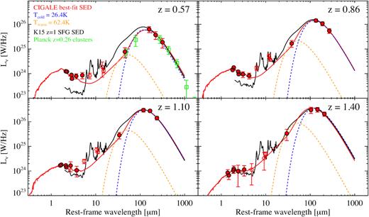
The best-fitting CIGALE SEDs (the red solid line) of our ‘total light’ cluster stacks (the red data points) in four redshift bins. Closed data points were used in the SED fitting, while open data points are excluded. For reference, we show the Kirkpatrick et al. (2015) SED for SFGs at z ∼ 1 (black) normalized to the longest wavelength data point. In the upper left-hand panel, stacked photometry from the Planck cluster sample (z ∼ 0.26, Planck Collaboration XLIII 2016) scaled down by a factor of 6 are shown as the open, green squares. The orange- and blue-dashed curves in each panel show the warm and cold dust components from a two-temperature modified blackbody fit where the temperatures are fixed to those used in the K15 model but the normalizations are free. The ratio of Lcold/Lwarm is 1.7–4.3 for the total cluster light compared to 1.4 for the K15 SED, suggesting more cold dust in the cluster stacks compared to typical massive galaxies.
In the upper left-hand panel of Fig. 10, we compare the SED for our lowest redshift bin to ‘total light’ stacks for a cluster sample at z ∼ 0.3 from Planck Collaboration XLIII (2016), scaled down by a factor of 6. Selected via SZ signal (Planck Collaboration 2014), this work stacked 645 clusters at 60 and 100 |$\, \mu$|m from IRAS and 350 |$\, \mu$|m – 3 mm using Planck imaging. Though this cluster sample is more massive than ours (M|$_{200}\sim 5\times 10^{14}\, \mathrm{M}_{\odot }$| for the Planck sample) and at a lower redshift, we find excellent agreement in the shape of the far-IR SED, including the relative dearth of warm dust emission. We discuss the reason for the lack of warm dust, or excess of cold dust further in Section 5.1.
4.3 Comparison of ‘total light’ cluster stacking to individual galaxy stacking in the far-infrared
In the previous sections, we used a ‘total light’ stacking technique to push down the luminosity function to get a more complete accounting of the total IR light coming from massive clusters. In this section, we use the spectroscopic and robust photometric redshifts available for this cluster sample to tease out the contributions to the total far-IR (i.e. the cold dust) from different cluster populations. Namely, we performed stacking at 250 |$\, \mu$|m on individual, known cluster members in bins of stellar mass.
Individual galaxy stacking is done following the procedure from Alberts et al. (2014), with minor updates that are summarized here. Cluster membership is determined from a mass-limited galaxy catalogue (|$80{{\ \rm per\ cent}}$| complete at log M⋆/M⊙ = 10.1) using full photometric redshift probability distributions (Eisenhardt et al. 2008; Chung et al. 2014). Cluster galaxies within 1 Mpc of the cluster centres are then sorted into the same redshift bins as our ‘total light’ stacking in two bins of stellar mass (|$10.1\lt \mathrm{log}\, M_{\star }/\mathrm{M}_{\odot }\lt 11$| and log M⋆/M⊙ > 11). Finally, the Herschel/SPIRE 250 μm image is stacked at their positions. A radius of 1 Mpc is chosen for this analysis in order to negate the need for beamsize and centroiding corrections when comparing to the total light stacks (Section 4.1.1).
As discussed in Alberts et al. (2014), two corrections are then applied to the individual galaxy stacks. First, a baseline correction is applied to account for flux boosting as a result of the large SPIRE beamsize. This boosting is a strong function of galaxy density (Viero et al. 2013). The baseline signal to be removed is determined through stacking random pixels along the line of sight to the clusters (see Alberts et al. 2014, for more details). We update this correction from how it was done in our previous study to incorporate an approximation of the cluster light profile determined from this work: the random pixels stacked are drawn from a normal distribution with a FWHM determined via fitting a Gaussian to our ‘total light’ cluster stacks (Fig. 3). As discussed in Section 3.1.6, the IR profile of our clusters has a weak or no dependence on redshift and a FWHM|$\, = 600\,$|kpc is adopted for this correction in all bins. The effect of this updated procedure is to increase the correction for flux boosting, particularly for stacks out to large radii (the correction is increased relative to Alberts et al. (2014) by a factor of 2-3 for an aperture of |$r\sim 1\,$|Mpc), by more properly weighting the galaxy distribution towards the centre of the cluster (see Appendix C for more details). Secondly, a field correction, which mitigates contamination from field galaxies due to photometric redshift uncertainties, is applied as described in Alberts et al. (2014).
These corrected stacks measure the contribution to the cold dust emission at observed 250|$\, \mu$|m from massive (log M⋆/M⊙ > 10.1) cluster galaxies. By ratioing these stacks to the ‘total light’ cluster stacks (Fig. 11), we find that high mass (log M⋆/M⊙ > 11) and intermediate mass (|$10.1\lt \mathrm{log}\, M_{\star }/\mathrm{M}_{\odot }\lt 11$|) cluster galaxies each make up 10-20|${{\ \rm per\ cent}}$| of the total cluster light with no discernible redshift trend given our uncertainties. This analysis demonstrates that studies of massive cluster galaxy populations are probing only a fraction of the dust-obscured activity in massive clusters. Further implications of this result are discussed in Section 5.2.

The ratio of the infrared luminosity density contributed from intermediate (|$10.1\lt \mathrm{log}\, M_{\star }/\mathrm{M}_{\odot }\lt 11$|; purple circles) and high (log M⋆/M⊙ > 11; orange diamonds) mass galaxies to the total IR derived from ‘total light’ stacking for cluster galaxies as a function of redshift. We compare our cluster results to the field values in the same mass bins derived from deep Herschel imaging (teal and red lines with hatched uncertainty; Viero et al. 2013) and the SIDES simulation (blue and orange lines with solid uncertainty; Béthermin et al. 2017). The shaded solid/hatched regions represent the uncertainty and scatter on this ratio; for the SIDES simulation, this is based on the known uncertainties on the simulation inputs and is likely an underestimate of the true scatter (see Section 5.3 for further details). Although the high mass cluster galaxies agree well with the field ratios at comparable mass, the intermediate mass cluster galaxies sit well below the expected contribution to the total IR from similar mass galaxies in the field.
5 DISCUSSION
5.1 Total dust emission in clusters
In Fig. 10, we showed that the total cluster SEDs have relatively more cold dust than warm dust in the far-IR compared to what is seen in massive galaxies in our three lower redshift bins, with a slightly warmer SED the highest redshift bin. At z ∼ 0.6, our SEDs are consistent with the on average cooler stacked SEDs found in an independent study of 645 low-z SZ-selected clusters from the Planck team (Planck Collaboration 2016). These total cluster stacks contain all galaxies, low- and high-mass, as well as ICD. We expect from numerous studies that the ICD component is minimal (Bai, Rieke & Rieke 2007; Chelouche, Koester & Bowen 2007; Giard et al. 2008; McGee & Balogh 2010; Gutiérrez & López-Corredoira 2014, 2017; Longobardi et al. 2020); for example, Bianchi et al. (2017) measured an upper limit on the 250 μm emission in Virgo as |$I_{250}\sim 0.1\,$| MJy sr−1, which would be a negligible contribution to our stacks. This leaves the galaxy component to dominate the SEDs. Alberts et al. (2016) found that massive cluster galaxies fit well to the warmer K15 empirical template found for similarly massive field galaxies and in Fig. 11 we demonstrate that the massive (log M⋆/M⊙ > 10) dusty galaxies contribute 20–30 per cent of the total IR emission. This indicates that 70–80 per cent of the IR light is likely originating from lower mass (log M⋆/M⊙ < 10) cluster galaxies. Given this, a colder spectrum is expected from the known dust luminosity–temperature relation for the field: |$T_{\rm {dust}} \propto L_{\rm IR}^{0.06}$| for nearby IR luminous galaxies (Casey et al. 2014). This relation implies that galaxies which are 100 times less luminous in the IR will have dust temperatures that are 1.3 times lower. The luminosity-weighted dust temperature of K15 SED is ∼42 K, whereas we get 30–36 K for the cluster stacks (Table 6), with a possible trend towards warmer temperatures in our highest redshift bin that may be due to i.e. increasing AGN activity (Martini et al. 2013; Alberts et al. 2016) and/or changing dust properties. Therefore, the cooler SEDs for the cluster stacks are consistent with the dominant contribution from the lower luminosity, cooler galaxies. While we do not need to invoke ICD to explain the cooler SED, we cannot rule out a contribution from ICD to the total cluster SEDs.
Quite a different picture emerged from a recent study of 179 Subaru-selected proto-clusters at z ∼ 4 (Kubo et al. 2019), where similar total light measurements were made. While the z < 1.6 clusters show a prominent cool dust component with less warm dust than even typical (high mass) high-z SFGs, the z ∼ 4 proto-clusters exhibit an excess in the mid-IR that would require intense starbursts and/or AGN heating. Simulations predict that proto-clusters at z ∼ 4 are characterized by active growth with a high contribution to the total SFR density at those epochs (Chiang et al. 2017). Additionally, we have evidence that AGN activity within the massive cluster galaxy population increases with redshift up to z ∼ 2 (Martini et al. 2013; Alberts et al. 2016), which may be influencing the warmer SED in our highest redshift bin. In general, the gas needed to fuel intense starbursts and AGN – and propel them to dominate the total cluster light – will have diminished from the proto-cluster to the cluster regime (e.g. Liu et al. 2019); direct progenitor samples will be vital to tracing this evolutionary history.
We can gain further insight into what is dominating the far-IR light in high-z clusters by looking at its distribution relative to the stellar light. In Figs 7 and 8, we showed via the (corrected) radial profiles that the dust emission is similarly extended as the stellar mass distribution, but that the dust emission is suppressed in the core relative to the much stronger peak in the stellar light. This is expected at lower redshifts (i.e. Chung et al. 2011, at z ∼ 0), where, for example, Rodríguez-Muñoz et al. (2019) found a suppression of star formation and a decrease in the SSFR of massive galaxies in the cores of clusters from z = 0.2−0.9, which they attributed to slow environmental processes such as strangulation. Extending this analysis for obscured star formation in massive cluster galaxies up to z = 1.75, Brodwin et al. (2013) and Alberts et al. (2016) found that this suppression appears to reverse, on average, at z ∼ 1.4, suggesting a transition epoch dominated by a fast quenching mechanism. These studies, however, also noted strong cluster-to-cluster variation within relatively small cluster samples (∼10–15), stressing the need for measurements averaged over large cluster samples. In this work, we have averaged the total light – again dominated by the low mass cluster constituents (Fig. 11) – over ∼40–80 clusters per redshift bin, finding that the IR suppression is evident, on average, up to z ∼ 1.6.
Even though we find that the dust emission is, on average, less centrally concentrated than the stellar light in our cluster sample, the far-IR radial profiles are still best-fit by a relatively high concentration NFW profile. This appears to be inconsistent with studies that find that blue SFGs usually have lower concentrations than their quiescent counterparts (van der Burg et al. 2014; Hennig et al. 2017). Since these studies probed massive galaxies, one explanation could be that lower mass SFGs, which dominate the total IR signal in the clusters, are more centrally concentrated, while higher mass SFGs are less concentrated, potentially due to preferential quenching at small radii. To test this, we repeat the analysis discussed in Section 4.3 – stacking massive galaxies individually, then ratioing this to the total light cluster stacks – while masking out the central 200–300 kpc, to determine the fraction of cluster IR light contributed by massive galaxies relative to the total outside of the regime where we see IR suppression. If massive cluster SFGs are less centrally concentrated, we would expect to find a higher fractional contribution to the total cluster IR light with the core masked. However, we find that the fraction contributed outside of the core is consistent with the fraction including the core, within the uncertainties. It is therefore unlikely that the IR suppression in the cluster cores is driven solely by the preferential quenching of massive cluster SFGs. Centrally concentrated low mass cluster SFGs are also likely being quenched, in agreement with recent studies which show environmental quenching of low-mass (log M⋆/M⊙ < 10) galaxies ramps up quickly at z < 1.5 (Kawinwanichakij et al. 2017). We note a potential alternative explanation for the difference in concentration: previous works that found a low concentration for cluster SFGs based on (optically) blue colours were not accounting for the obscured star formation component, which dominates in high-mass galaxies at these redshifts (Madau & Dickinson 2014; Whitaker et al. 2017), and may be particularly relevant in overdense environments, even at low masses (see Section 5.3).
5.2 The decline of total obscured star formation activity in clusters
In Section 4.2, we derived the total SFRIR enclosed in the virial radius (|$R_{200} = 1\,$|Mpc) from our best-fitting SEDs (Table 6), assuming a likely negligible contribution from ICD based on the literature, which has obtained mostly upper limits (Chelouche et al. 2007; Bai et al. 2007; Giard et al. 2008; McGee & Balogh 2010; Gutiérrez & López-Corredoira 2014, 2017, but see Longobardi et al. (2020)). We found a dramatic 8-fold decrease in the obscured star formation from z ∼ 1.4 to z ∼ 0.6, a strong evolution that mirrors the evolution of the average SFRIR found for massive cluster galaxies (Alberts et al. 2014).
Fig. 12 combines the total stellar mass with SFRIR to examine the evolution of the ‘total light’ SSFR as a function of redshift. We compare this evolution to that measured for massive galaxies only through both mid-IR detections of individual cluster galaxies (teal open circles; Brodwin et al. 2013) and far-IR stacking (teal solid line and squares; Alberts et al. 2014, this work). We find that there is a remarkably similar evolution between the total and massive galaxy only SSFRs, with a similar rate of decline towards lower redshifts. Fig. 12 shows that the SSFRs of massive cluster members (teal squares) are on average a factor of 2 below the total light SSFRs (the red squares). This implies that the log M⋆/M⊙ < 10 cluster galaxies will be on average a factor of 2 higher. This is roughly consistent with the trend of SSFR with stellar mass observed for field galaxies (Whitaker et al. 2014), with the caveat that the field measurements were made for SFRUV + IR, with the UV component expected to be significant for the low-mass galaxies (Whitaker et al. 2017). We additionally note that the bootstrapped uncertainties for the ‘total light’ SSFR are large (0.2–0.5 dex), which likely includes the significant cluster-to-cluster variation that has been observed before (i.e. Brodwin et al. 2013; Alberts et al. 2016).
The SSFR enclosed in |$1\,$| Mpc as a function of redshift, derived from our ‘total light’ stacks using Spitzer and Herschel data to measure the total stellar mass and obscured SFRs, respectively. We compare these results to trends found for massive cluster galaxies (log M⋆/M⊙ > 10.1) determined via SPIRE stacking (the teal solid line and the squares; Alberts et al. 2014, this work) and from individual detections via deep mid-IR imaging (the teal open circles; Brodwin et al. 2013). The SSFR–z relation for field galaxies with log M⋆/M⊙ > 10.1 is shown as the dotted black line (Alberts et al. 2014). The shaded region denotes the main sequence (Whitaker et al. 2014) for field galaxies at fixed stellar mass (log M⋆/M⊙ = 10) for reference. The ‘total’ cluster SSFRs have a steeper evolution than comparable field populations, but reach field-like levels at z ∼ 1.5, in agreement with studies of massive cluster galaxies. This shows that the high and low mass cluster members are undergoing similar evolution in clusters at this epoch.
Fig. 12 further compares the evolution of the total and massive cluster SSFRs to field measurements: stacked field galaxies with log M⋆/M⊙ > 10.1 (the dotted black line; Alberts et al. 2014) and the main sequence at fixed mass (log M⋆/M⊙ = 10, the solid/dashed black line and the shaded region; Whitaker et al. 2014). Relative to the field, the total cluster measurements are comparable in star formation activity per unit stellar mass at the highest redshift bin probed (z ∼ 1.3−1.6), with rapid quenching below the field level thereafter. This result reveals that the transition epoch around z ∼ 1.4 for massive galaxies in clusters from abundant star formation to significant quenching found in previous studies (Brodwin et al. 2013; Alberts et al. 2014, 2016) also holds for the lower mass galaxies probed by the total cluster measurements.
Which cluster galaxies are driving the evolution in the total obscured cluster activity? In addition to massive cluster galaxies SSFRs being roughly a factor of 2 lower than that of the total cluster SSFRs, in Fig. 11 we showed that intermediate (|$10.1 \lt \mathrm{log\, } M_{\star }/\mathrm{M}_{\odot }\lt 11$|) and high (log M⋆/M⊙ > 11) mass cluster galaxies together only account for a minority (|$\sim 20\!-\!30{{\ \rm per\ cent}}$|) of the far-IR emission in these clusters at any redshift probed in this work. Given the similar evolution with redshift between the total and massive cluster galaxies in SFR and SSFR, this indicates that low mass (log M⋆/M⊙ ≲ 10) cluster galaxies are experiencing quenching alongside their massive cousins during this epoch. This result is consistent with recent literature which has examined the quenched fraction and environmental quenching efficiency – the fraction of cluster galaxies that would be forming stars in the field – down to similarly low masses. Work based on nearest neighbor techniques in the ZFOURGE survey (Straatman et al. 2016) found that the environmental quenching of low mass (log |$M_{\star }/\mathrm{M}_{\odot }\sim 9.0 \, (9.5)$| at |$z\sim 1.3\, (2)$|) galaxies in overdense regions is very inefficient at z ≳ 1.5, but ramps up quickly at lower redshifts (Kawinwanichakij et al. 2017). Using the same sample and studying the stellar mass function (SMF) of quiescent cluster galaxies, Papovich et al. (2018) demonstrated that environmental quenching must be mass dependent at high redshift, with the efficiency of quenching low-mass galaxies in overdense regions growing between z ∼ 1.5 and z ∼ 0.5, in order to match the faint end of the SMF. A study of more massive clusters (log M200/M⊙ ∼ 14−15) found a similar ramp up in the faint end of the red sequence (RS), with a distinct deficit in faint RS galaxies at z ∼ 1–1.3 followed by a factor of 2 growth by z ∼ 0.6 (Chan et al. 2019). This ramp up may complete by z ∼ 0.6; van der Burg et al. (2018) found that the environmental quenching efficiency in massive clusters was independent of stellar mass at fixed radius down to log M⋆/M⊙ ∼ 9.5. Together with this work, the emerging picture is that the environmental quenching of low mass (log M⋆/M⊙ < 10) galaxies at z ≲ 1.5 is a significant driver of cluster galaxy evolution.
5.3 The low-mass contribution to the total far-infrared emission
To further shed light on the nature of low mass cluster galaxies, we compare the contribution from massive galaxies to the total IR light to two studies which quantify this ratio for the field (Fig. 11). First, we compare to deep blank field Herschel observations. Viero et al. (2013) used unbiased stacking methods on K-band selected galaxy catalogs to estimate the contribution to the cosmic infrared background (CIB) from various populations. This includes mass-limited galaxy samples down to log M⋆/M⊙ = 9, below which low-mass field galaxies are expected to contribute little to the CIB (|$\lt 30{{\ \rm per\ cent}}$| of their SFR is obscured; Whitaker et al. 2017). The observational results of this field study are that intermediate mass (|$10 \lt \mathrm{log\, } M_{\star }/\mathrm{M}_{\odot }\lt 11$|) field galaxies dominate the CIB at 250 |$\, \mu$|m (|$65\pm 9{{\ \rm per\ cent}}$|), with high-mass galaxies contributing a minimal amount (|$8\pm 1{{\ \rm per\ cent}}$|), up to z ∼ 4.
Secondly, we compare to the predicted field properties from the publicy available Simulated Infrared Dusty Extragalactic Sky (SIDES; Béthermin et al. 2017). This simulation provides a 2 deg2 blank field of log Mhalo/M⊙ ∼ 10−12 DM haloes, which are populated with galaxies via abundance matching and observed stellar mass functions. Galaxy IR properties are then assigned using the 2SFM galaxy evolution model (Sargent et al. 2012; Béthermin et al. 2012, 2013) and the Magdis et al. (2012) SED library. The resulting catalog8 provides the 250 |$\, \mu$|m flux densities for galaxies down to log M⋆/M⊙ = 8. The SIDES predicted ratio of the luminosity density contributed by intermediate- and high-mass galaxies to the total is shown in Fig. 11, with the shaded regions representing the combined input scatter into the simulation for the MS (0.3 dex; Ilbert et al. 2015; Schreiber et al. 2015) and the SED library (0.2 dex in <U >; Magdis et al. 2012), which will directly affect the 250 |$\, \mu$|m flux. We caution that this simulation extrapolates to low mass and low LIR, a regime that is not well constrained observationally, and so the uncertainty is likely larger than depicted. To first order, the SIDES simulation agrees with the observed contributions to the CIB from Viero et al. (2013) at each of these two stellar mass bins.
This comparison to the field reveals that high mass (|$\mathrm{log\, } M_{\star }/\mathrm{M}_{\odot }\gt 11$|) cluster and field galaxies have similar (minimal) contributions to the total IR budget. With our data set, it is difficult to disentangle mass- and environmental-quenching in this case. The difference between the cluster and field intermediate mass (|$10.1 \lt \mathrm{log\, } M_{\star }/\mathrm{M}_{\odot }\lt 11$|) galaxies, on the other hand, is striking and suggests significant environmental differences. Compared to the percentage in the field (|$65\pm 9{{\ \rm per\ cent}}$|), intermediate mass clusters galaxies only account for |$15\pm 5{{\ \rm per\ cent}}$| (averaged over our redshift bins) of the total IR output, a factor of 4 deficit. This low fractional contribution at all redshifts is puzzling. By z ∼ 0.6, we expect that a large fraction of intermediate mass cluster galaxies have quenched (i.e. Muzzin et al. 2012; Nantais et al. 2017); however, as discussed earlier, lower mass cluster galaxies are also quenching, such that at least one study finds no mass dependence for the quenching efficiency at this epoch (van der Burg et al. 2018). At the high redshift end of our sample, the low fractional contribution suggests that intermediate mass galaxies largely quenched earlier than z ∼ 1.5. This has not, however, been found to be the case in the literature. A recent look at the environmental quenching efficiency as a function of redshift for log M⋆/M⊙ > 10.3 cluster galaxies (Nantais et al. 2017) found that while the quenched fraction is |$80{{\ \rm per\ cent}}$| by z ∼ 1.3, rising to |$88{{\ \rm per\ cent}}$| at z < 1.1, it is only |$42{{\ \rm per\ cent}}$| at z ∼ 1.6, consistent with the quenched fraction in the field (see also van der Burg et al. 2013). This decrease in environmental quenching efficiency is congruous with the findings of field-like SF activity at these high redshifts (Brodwin et al. 2013; Alberts et al. 2014, 2016) and together these different approaches suggest that intermediate mass galaxies should contribute significantly to the IR budget in clusters.
Further complicating the picture at high redshift is that the total cluster SSFR is within a factor of ∼3 (given the 1σ uncertainty) of the field activity, suggesting that minimal SF activity is “missing”, assuming there is no strong reversal of the SFR–density relation. Yet if the intermediate- (and high-) mass cluster galaxies are quenched at earlier times, then at z ∼ 1.4 the observed SF must be provided by a population that does not provide it in the field. This could be solved with a significantly different ratio of low to intermediate-/high-mass SFGs in clusters than in the field; however, studies of the star-forming SMF in low- versus high-density environments find them to be remarkably similar (van der Burg et al. 2013; Papovich et al. 2018). Alternatively, low-mass cluster SFGs could have enhanced SFRs. Studies of low-mass cluster galaxies, however, typically find they reside on or below the main sequence (Old et al. 2020), though we note that these studies often do not directly trace the obscured component.
There is a third possibility: the mode of star formation in cluster galaxies is different than in the field without being enhanced; that is, that cluster galaxies are dustier than their field equivalents (Koyama et al. 2011; Hatch et al. 2016; Sobral et al. 2016). Overdensities of DSFGs are increasingly being found to be signposts for proto-clusters at z ≳ 2 (i.e. Casey 2016; Kato et al. 2016); however, there have been few studies looking at the dust content in clusters relative to field galaxies at the epoch relevant to this study. Hatch et al. (2016) found an excess of red galaxies in the main cluster (log M200/M⊙ = 13.76) forming in a proto-cluster at z = 1.6. Using SED fitting and MIPS 24|$\, \mu$|m photometry, they determined that this excess is comprised of both passive cluster members and DSFGs, with the DSFGs occurring at a rate of three times that found in group and field environments. Though they did not establish a mass dependence for this red excess of DSFGs, they found it extended to their low-mass cut-off (log M⋆/M⊙ > 9.7). Accounting for their selection effects – biased particularly against faint, red galaxies – they estimated an upper limit for the red fraction at their low-mass end, which could accommodate an additional factor of 2 in low-mass DSFGs in the cluster environment. This finding of excess dust may be indirectly corroborated by studies showing enhanced gas fractions (Mok et al. 2016; Noble et al. 2017, 2019; Hayashi et al. 2018), assuming similar dust/gas ratios, and enhanced gas-phase metallicities in overdense environments both locally and at high redshift (Ellison et al. 2009; Peng & Maiolino 2014; Maier et al. 2019a,b; Franchetto et al. 2020).
In summary, the behaviour of the total cluster SSFR, particularly at high redshift, and the low fractional contribution of intermediate-mass cluster galaxies to the total IR budget likely indicates that multiple effects are at play. We posit that mass-dependent environmental quenching which evolves with redshift plus a more obscured mode of SF in lower mass cluster galaxies may be required to explain the behaviour of the total far-IR emission in clusters. We note that throughout this section, we have relied on the obscured SFR and SSFR, meaning the unobscured component is unaccounted for. If low-mass cluster galaxies have largely unobscured SF like field galaxies (Whitaker et al. 2017), this component may be significant and boost the SSFR even more relative to the field at high redshift. Measuring the unobscured component in addition to the dust mass directly are key to disentangling these effects. We discuss the prospects for this in Section 5.6.
5.4 Stellar-to-halo-mass ratios
Here we discuss the stellar mass content of clusters with respect to their DM content, a ratio determined by the balance between the assembly of DM and externally formed stars, as well as in situ star formation. As mentioned in Section 2.1, based on clustering measurements, the mean halo mass of our cluster sample is about 1013.8 M⊙ with no significant redshift evolution (Brodwin et al. 2007; Lin et al. 2013; Alberts et al. 2014); in other words, our cluster samples should be treated as roughly fixed mass, rather than as an progenitor sample. Accordingly, the total stellar mass per cluster based on the full SED fitting (constrained primarily by the near-IR WISE and Spitzer bands) is also roughly constant over the four redshift bins (Table 6). This gives a total stellar-to-halo-mass ratio, M⋆/Mhalo, of about 1–3|${{\ \rm per\ cent}}$| for our clusters as shown in Fig. 13. The left-hand panel shows the lack of a significant redshift evolution of this quantity for our clusters, while the right-hand panel shows the trend of M⋆/Mhalo with halo mass, with additional measurements from more massive cluster samples over a similar redshift range (Hilton et al. 2013; van der Burg et al. 2014; Chiu et al. 2018; Decker et al. 2019).
The average total stellar to halo mass ratios M⋆/Mhalo as function of redshift (left-hand panel) and halo mass Mhalo = M200 (right-hand panel). The circles in both panels show the measurements for our cluster sample of roughly constant halo mass (log M200/M⊙ = 13.8) in four redshift bins, with the total stellar masses constrained by the SEDs of the ‘total light’ stacks (Fig. 10; Table 6). For comparison, we show the semi-analytic model predictions from Henriques et al. (2015) and Guo et al. ( 2013) in the left-hand panel, and Henriques et al. (2015) in the right-hand panel. The cyan dash–dotted line on the right-hand panel shows the observed relation for an X-ray selected cluster sample at z = 0 from Gonzalez et al. (2013). Literature measurements for several more massive cluster samples at 0.5 ≲ z ≲ 1 are also shown on the right-hand panel with various symbols as labeled.
As our stacking measurements capture the stellar mass content in not only the central but also satellite galaxies and intracluster stars, it is insufficient to compare our result with the often referenced stellar mass–halo mass relations for central galaxies (e.g. Moster et al. 2010). Instead, we extract and show in Fig. 13 the total stellar mass–halo mass ratios predicted in the semi-analytic galaxy models of Henriques et al. (2015, solid lines) and Guo et al. (2013, dashed line) coupled with the Millennium suite of cosmological N-body simulations (Springel et al. 2005). In the left-hand panel, the model predictions are extracted by selecting the most massive clusters in the |$\sim (500/h\ \rm Mpc)^3$| simulation box down to a redshift-dependent mass threshold chosen such that the mean halo mass of the sample is a constant at log M200/M⊙ = 13.8. This selection is designed to mimic that of our observations. Overall, we see slightly different M⋆/Mhalo versus redshift for the mass-matched clusters in the two models due to different implementations of quenching, while both models are still consistent with our measurements for observed clusters within the errors. We also extract the halo mass dependence of M⋆/Mhalo predicted in the Henriques et al. (2015) model at z = 1 and z = 0 shown in the right-hand panel of Fig. 13 using the dark and light grey solid lines, respectively.
In addition to the M⋆/Mhalo measurements shown from this work and the literature, we also compare the M⋆/Mhalo versus halo mass relation estimated for a sample of X-ray selected clusters at z ∼ 0 from Gonzalez et al. (2013) in the cyan dash–dotted line. The Henriques et al. (2015) model predicts a relatively weak relation between M⋆/Mhalo and halo mass compared to that observed at z = 0 in Gonzalez et al. (2013). From the data compiled it is difficult to distinguish these cases; the constraining measurements from the literature shown suggest a steep slope but unfortunately our cluster sample supports both scenarios with large uncertainties. Providing constraining anchors at additional halo masses will have important implications for how environmental quenching is implemented in the models. Improvements in the empirical measurements will come from wide-area cluster surveys that span very large dynamical ranges in halo mass. For instance, the all-sky MaDCoWS survey (Gonzalez et al. 2019) contains thousands of z ∼ 1 groups and clusters with both IRAC and WISE imaging spanning a halo mass range of |$13.2 \lesssim \log {M_{\rm halo}/\mathrm{M}_\odot } \lesssim 15.2$|. This will allow for uniform measurements of both (richness-based) halo and stellar masses, thus minimizing systematic errors along the halo mass axis. The 1500 deg2 SPT-3G cluster survey (Benson et al. 2014), though limited to masses above ∼1014 M⊙, will provide accurate SZ masses for all systems. These and other wide-area surveys will much better constrain the M⋆/Mhalo versus halo mass relation at high-z.
5.5 The concentration of the total stellar mass in intermediate mass clusters at z ∼ 0.5−1.6
In Section 4.1, we presented the ‘total light’ averaged radial flux profiles for our cluster stacks in four redshift bins and across our wavelength bands. We compare our results to a fiducial model, a projected NFW profile (Navarro et al. 1996), which has been shown to describe the cluster stellar mass distribution (e.g. Lin et al. 2004; Muzzin et al. 2007; van der Burg et al. 2014; Hennig et al. 2017; Lin et al. 2017). From fitting an NFW profile to the (corrected) 3.6|$\, \mu$|m radial profile – which probes λrest = 1.5−2.3 for our sample and therefore is expected to scale linearly with stellar mass – we found our profiles heavily favour scale lengths of |$r_s = 0.13\!-\!0.15\,$| Mpc, corresponding to a concentration of c ≈ 7, with no significant redshift evolution across our sample.
Only a handful of concentration parameter measurements exist in the literature at similar redshifts, based on individual galaxy distributions. van der Burg et al. (2014) used a K-band-selected catalogue to look at the stellar mass radial profile in ten z ∼ 1 clusters with a typical mass of log M200/M⊙ ∼ 14.3. They found a similar high concentration of c ∼ 7 for massive (individually detected) galaxies. Using SPT–SZ (Story et al. 2013) clusters, Hennig et al. (2017) found hints of high concentrations (c ≈ 5−10) in their stacked number density radial profiles at z ∼ 0.8−1 for log M200/M⊙ ∼ 14.8 clusters, and noted only statistically weak trends with redshift and no significant trend with halo mass as well as a large scatter in individual cluster profiles. In contrast, Lin et al. (2017) found c ∼ 3 for z ∼ 1 HSC–SSP clusters with comparable masses to the van der Burg et al. (2014) sample. Additional studies at z ∼ 1 find concentrations of c ≈ 3−4 for more massive cluster samples (log M200/M⊙ ≳ 14.5−15; Capozzi et al. 2012; Zenteno et al. 2016).
In this work, we have used a uniformly selected cluster sample to produce radial profiles at near fixed halo mass (Section 2,4.2) over a range of redshifts. We note that averaging via stacking reduces the influence of sub-structure on the measured concentration (Gao et al. 2008). The uniformity of our radial profiles and high measured c values at a range of redshifts suggests that halo mass, rather than redshift, is the dominant factor in determining the stellar mass concentration. This is consistent with progenitor studies – which indicate c evolves strongly with cluster growth (van der Burg et al. 2015) – and with the generally lower concentrations found for more massive clusters at low redshift (i.e. Lin et al. 2004; Muzzin et al. 2007; Budzynski et al. 2012) and up to z ∼ 1 (Capozzi et al. 2012; Zenteno et al. 2016; Lin et al. 2017).
Observations of the DM profiles of clusters via lensing and X-ray imaging have found a steep dependence of cDM on the halo mass (Sereno & Covone 2013; Amodeo et al. 2016). This dependence, however, has not been been reproduced in the studies of stellar mass or galaxy number density concentrations where a range of halo masses are available (i.e. Budzynski et al. 2012). Simulations have similarly not yet converged on what detailed effects baryons have on the total concentration in high-mass systems (i.e. Gnedin et al. 2004; Duffy et al. 2010; De Boni et al. 2013). A strict halo mass dependence would, for example, put our results at odds with the van der Burg et al. (2014) results; however, this is again not a fair comparison as ‘total light’ stacking is probing a different population than that which requires individual galaxy detections. In order to reconcile observed cluster concentrations and inform simulations, more uniform cluster selection and depth of observations is needed to compare like populations and dynamical states over a range of halo masses. Techniques such as stacking further minimize cluster-to-cluster variations such as sub-structure, stressing the importance of large samples.
5.6 Implications and prospects for future studies
5.6.1 The total unobscured star formation in massive clusters
Throughout this work, we have probed the far-IR as a proxy for (obscured) star formation. For massive field galaxies near cosmic noon, the obscured component dominates the SFR budget in SFGs; however, lower mass field galaxies are found to have a lower fraction of their star formation obscured by dust (|$f_{\rm {obscured}} = \rm {SFR_{IR}\, /\, SFR_{UV+IR}} = 0.5$| for galaxies with |$\mathrm{log}\, M_{\star }/\mathrm{M}_{\odot }= 9.4$|; Whitaker et al. 2017). Our results (Fig. 11) show that the total far-IR cluster stacks are dominated by lower mass, lower luminosity galaxies (|$\mathrm{log}\, M_{\star }/\mathrm{M}_{\odot }\lt 10$|, equivalent to SFR|$\, \lesssim 10\, M_{\odot }/\rm {yr}$| for main-sequence galaxies at z ∼ 1, Whitaker et al. 2014). If this low mass cluster population follows the field in terms of dust properties, this predicts a significant unobscured SF component which must be added to the total SF budget. If, on the other hand, cluster galaxies are dustier than their field counterparts (as discussed in Section 5.3), this component will be limited. An adaption of our stacking technique to work with GALEX UV data, which directly probes unobscured SF, will be presented in future work for the Boötes cluster sample and other (proto-)cluster surverys.
5.6.2 Quantifying the dust mass and gas content in large (proto-)cluster samples
The results in this work demonstrate that the far-IR component provides vital information about cluster evolution for high-z clusters. However, as shown in Fig. 10, our current data does not extend much beyond |$250\, \mu$|m in the rest-frame for clusters at z > 1. The longer (sub-)millimeter wavelengths are a very clean tracer of the total dust mass, a proxy for the total ISM mass assuming constant gas-to-dust ratios (e.g. Scoville et al. 2014). While ALMA has the sensitivity to detect massive, IR-luminous galaxies individually in high redshift (proto-)clusters (i.e. Noble et al. 2017; Zavala et al. 2019), it is inefficient at mapping the large areas needed to survey a large sample of (proto-)clusters. The Large Millimeter Telescope in Mexico will soon welcome a powerful new instrument, TolTEC, which will simultaneously image the sky at 1.1, 1.4, and 2.1 mm (Bryan et al. 2018). The project is planning to complete four public legacy surveys in 2020–2022, including two extragalactic surveys (Pope et al. 2019). The Large Scale Structure Survey will cover 50 square degrees over several multiwavelength data rich fields including the Boötes field. With 5 arcsec spatial resolution at 1.1 mm, the confusion noise is greatly reduced compared to previous single-dish millimeter surveys. We can apply our total light clusters stacking technique on the TolTEC maps to provide an anchor on the Rayleigh–Jeans tail of the dust distribution and constrain the dust masses. This will allow us to investigate how the total dust mass and radial dust mass distribution evolves in this Boötes cluster sample and compare to other cluster samples mentioned previously in this section.
5.6.3 Application to other (proto-)cluster samples
We have developed techniques to measure and compare the total light from samples of galaxy clusters over a large wavelength range. Our initial application of this technique is presented in this work for a large sample of clusters in the Boötes field, uniformly selected based on photometric overdensities of galaxies. This sample represents an excellent test case given the well-studied nature of this cluster sample, including an existing census of the massive dust-obscured galaxies (Brodwin et al. 2013; Alberts et al. 2014, 2016). Galaxy cluster surveys have long sought to understand the selection effects of various cluster samples from SZ, X-ray, and optical selections, and how a cluster’s halo mass is related to its evolutionary state. Our total light stacking technique can be applied to samples of clusters selected in different ways and with different masses to determine if the galaxy populations – including low-mass components – have similar radial distributions and obscured star formation properties (see discussions in Sections 5.1–5.3). Specifically, we plan to apply our technique to the large samples of clusters from the SPT (Story et al. 2013; Benson et al. 2014) and MaDCoWS (Gonzalez et al. 2019) surveys. These samples will greatly increase the dynamic range in halo mass analysed, reducing systematics when tracing the effects of halo mass on total stellar mass and concentration (see discussions in Sections 5.4–5.5). Furthermore, as was done in Kubo et al. (2019), this technique can extend the wavelength baseline into the near-IR for higher redshift proto-cluster samples such as those selected from the Planck survey (Planck Collaboration 2014, 2015). The results of these additional analyses will be presented in future papers.
6 CONCLUSIONS
‘Total light’ cluster stacking – the (background subtracted) summation of all light in a sample of clusters without regards to previously identified constituents – provides a look into cluster evolution that is complementary to the ongoing efforts that identify and study in detail (individually detected) sub-populations in small cluster samples. ‘Total light’ stacking provides an averaged view, marginalizing over sources of cluster-to-cluster variation (i.e. Geach et al. 2006; Alberts et al. 2016) such as sub-structure (Gao et al. 2008), while being significantly less sensitive to detection limits and the need for expensive spectroscopy. Specifically, this stacking technique currently provides the only method of analysing the lower mass, lower luminosity cluster components for large samples of (proto-)clusters; large samples being necessary to span a range of redshifts, halo masses, and dynamical states.
In this work, we presented our ‘total light’ stacking techniques for multiple wavelength regimes: the near- and mid-IR (via WISE and Spitzer) as well as the far-IR (via Herschel). We applied our techniques to a well-studied cluster sample at 0.5 < z < 1.6 in the Boötes field, using existing photometric redshifts and characterizations of the massive cluster population to check the robustness of our stacking and look at cluster populations over a range of redshifts.
Our main conclusions are as follows:
‘Total light’ stacking is a powerful tool for recovering extended cluster emission from the near- to far-IR even in the case of minimal ancillary data. Through existing large surveys, particularly all-sky coverage with WISE, these techniques are applicable to a much wider range of existing and future cluster surveys. For data sets where a significant fraction of sources are above the detection limit (i.e. the short wavebands of WISE and Spitzer), ‘total light’ stacking provides a lower limit on the total emission, which can then be corrected given cluster membership information. We provide our correction factors for WISE in Table 3, which can be used as a guideline for other cluster samples given the uniformity of the all-sky WISE coverage.
We measure the near-IR stellar light profiles, a direct proxy for the stellar mass distribution, using WISE and Spitzer for our clusters in four redshift bins spanning z = 0.5 to z = 1.6. The near-IR profiles drop off steeply, with the majority of the stellar emission enclosed in the virial radius (|$R_{200}\sim 1 \,$| Mpc). We find good agreement between the overlapping WISE and Spitzer filters. After applying appropriate corrections for centroiding uncertainties and beamsizes, we find that the near-IR profiles are well described by an NFW profile with a high concentration factor at all redshifts. We speculate that the uniform halo mass in our cluster sample is a driving factor behind this uniform concentration; however, a comparison with the literature highlights that the effect of baryons on the concentration is likely more complicated than a simple halo mass scaling relation.
Stacking in the far-IR reveals extended dust emission from (observed) 250–500|$\, \mu$|m with a profile that is remarkably similar to the stellar mass distribution except for the inner core (|$\lesssim 0.3\,$| Mpc), where the total dust emission is suppressed at all redshifts.
The ‘total light’ SED can be well described by a SFG model with a dearth of warm dust relative to massive field galaxies at z ≲ 1.3, with a slightly warmer SED in our highest redshift bin. This is in general consistent with the SED being dominated by low-mass, low-luminosity galaxies that are are found in the field to have colder SEDs than their massive cousins. No ICD is required to model the ‘total light’ SEDs; however, a minor contribution from ICD cannot be ruled out.
SSFRs derived from the ‘total light’ SEDs are found to evolve strongly with redshift, mirroring the evolution of the massive cluster members found in previous studies for this sample (Brodwin et al. 2013; Alberts et al. 2014, 2016). In our highest redshift bin, this SSFR is comparable to that expected in the field. A direct comparison of the IR luminosity density from massive (log M⋆/M⊙ ≳ 10) galaxies to the ‘total light’ shows that massive galaxies make up a minority (|$20\!-\!30{{\ \rm per\ cent}}$|) of the total cluster emission, consistent with the relatively cold SED. In particular, intermediate mass (log M⋆/M⊙ = 10−11) cluster galaxies contribute significantly less to the total IR light than is predicted for field galaxies. We discuss the possible origins of this difference, including quenching and excess dust in cluster environments.
The total stellar mass measured in our four redshift bins is flat with redshift. This is expected given the nature of our cluster sample, which, due to the selection technique, has a uniform halo mass at the different epochs explored. We compare the total stellar mass to halo mass ratio of our sample to predictions from semi-analytic models (Guo et al. 2013; Henriques et al. 2015) and N-body simulations (Springel et al. 2005). We find good agreement with the predicted M⋆/Mhalo value of 1–3 per cent.
‘Total light’ stacking can be extended to other wavelength regimes. The dominance of the low mass cluster galaxy population in the total dust emission measured in this work may imply that a substantial portion of the cluster star formation is unobscured and thus best measured in the UV. Complementary to this, large (sub-)millimeter imaging surveys will more directly probe the total cluster dust mass, enabling a comparison of the dust properties in clusters versus field and providing a proxy for gas content. Expanding the wavelength regimes covered and applying these stacking techniques to additional (proto-)cluster samples will be presented in future work.
ACKNOWLEDGEMENTS
The authors thank Denis Burgarella for advice on CIGALE, Carlotta Gruppioni for discussions about her IR luminosity functions, and Matthieu Bethermin for discussion about the SIDES mock catalogue. The authors additionally thank George Rieke, Mattia Vaccari, and David Shupe for insight into the Böotes MIPS imaging and Aaron Meisner, Dustin Lang, and Ned Wright for discussion regarding the WISE imaging. The authors acknowledge financial support from NASA through the Astrophysics Data Analysis Program, grant number 80NSSC19K0582. This publication has used data products from the Wide-field Infrared Survey Explorer, which is a joint project of the University of California, Los Angeles, and the Jet Propulsion Laboratory/California Institute of Technology, funded by the National Aeronautics and Space Administration. This work is based (in part) on observations made with the Spitzer Space Telescope, which was operated by the Jet Propulsion Laboratory, California Institute of Technology under a contract with NASA. The Herschel spacecraft was designed, built, tested, and launched under a contract to ESA managed by the Herschel/Planck Project team by an industrial consortium under the overall responsibility of the prime contractor Thales Alenia Space (Cannes), and including Astrium (Friedrichshafen) responsible for the payload module and for system testing at spacecraft level, Thales Alenia Space (Turin) responsible for the service module, and Astrium (Toulouse) responsible for the telescope, with in excess of a hundred subcontractors. This research has used the NASA/IPAC Infrared Science Archive, which is funded by the National Aeronautics and Space Administration and operated by the California Institute of Technology.
DATA AVAILABILITY STATEMENT
The WISE, Spitzer/IRAC, and Herschel data underlying this article are available in the NASA/IPAC Infrared Science Archive at irsa.ipac.caltech.edu. The Spitzer/MIPS data were provided by the MAGES team; access may be requested through the corresponding author and granted with permission from the MAGES team. Other data products generated in this article will be shared on reasonable request to the corresponding author.
Footnotes
Herschel is an ESA space observatory with science instruments provided by European-led Principal Investigator consortia and with important participation from NASA.
The 3-Band Cryo observations only cover a limited ecliptic longitudinal range, which excluded our survey field.
The monochromatic AB magnitudes of Vega are 2.699, 3.339, 5.174, and 6.620 in the W1, W2, W3, and W4 bands, respectively, according to the WISE All-Sky Data Release document found at http://WISE2.ipac.caltech.edu/docs/release/allsky/expsup/sec4_4h.html. We note that, for W4, this is within 0.04 mag of the zero-point found in Brown, Jarrett & Cluver (2014), based on an empirical recalibration that revised the effective wavelength to 22.8|$\, \mu$|m.
REFERENCES
APPENDIX A: COMPARISON OF DIFFERENT STACKING METHODS FOR WISE
We give a full description of the various tests we have conducted to quantify how different image processing procedures and stacking techniques can impact the stacked flux measurements. The same behaviour is observed in all bands, and here, we illustrate our results in the W2 band.
In Fig. A1, we show four different image stacks of the WISE W2 band on the cluster and off-cluster positions, all of which are performed on the z = 0.7−1.0 sample. The leftmost panels are mean_unmasked stacks, which are created by taking a pixel-wise mean of the _unmasked images. The second left column shows the mean_masked stacks where we mask out all sources present in the image. The third and fourth columns show the median_masked and median_sub images, respectively. The latter use the _sub images which are simply sky-subtracted images where all sources are present therein.
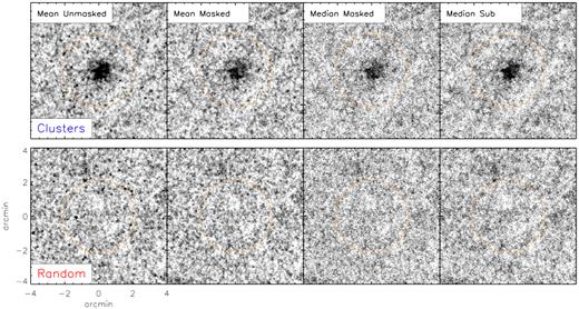
Results of our WISE W2 stacking analyses using the z = 0.7−1.0 sample are shown to illustrate the three stacking techniques we employ in this work as described in Sections 3.1.1 and 3.1.2. Top and bottom panels show the results of each method, labelled atop, performed on the cluster positions (top) and random positions (bottom). Each image is 8 arcmin on a side. In each panel, we show a circle of 1 Mpc radius at z = 0.86 as a dashed line.
In Table A1, we list the aperture fluxes measured from these images. We also show the sky properties measured in the cluster and off-cluster stack. For the latter, we list the mean value after 500 random measurements. We do not give the spread of the σp because it is consistent with zero in the adopted precision. It is evident that in all but the mean_unmasked stack the measured fluxes are consistent with one another within 15 per cent. The fluxes at large radii are somewhat sensitive to small changes in the assumed sky level. In particular, the agreement of the median_sub fluxes with the others is remarkable considering that the source density in the former is much higher than that in the latter. As noted previously (see Section 3.2), the mean_unmasked fluxes are expected to be higher than other versions as it should represent the total flux including those contributed by the photo-z cluster members.
z = 0.7–1.0 clusters: W2-band fluxes and noise properties of four different image stacks.
| Radius | mean_unmasked | mean_masked | median_masked | median_sub |
|---|---|---|---|---|
| (arcsec) | (μJy) | (μJy) | (μJy) | (μJy) |
| σp (cluster) | 0.148 | 0.130 | 0.140 | 0.147 |
| σp (off-cluster) | 0.149 | 0.131 | 0.131 | 0.131 |
| 5.50 | 14.0 (0.5) | 8.1 (0.5) | 8.2 (0.5) | 10.3 (0.5) |
| 11.00 | 47.8 (1.0) | 27.1 (0.9) | 26.4 (1.0) | 36.8 (1.0) |
| 16.50 | 92.9 (1.6) | 52.1 (1.4) | 54.5 (1.5) | 70.1 (1.5) |
| 22.00 | 143.7 (2.1) | 85.5 (1.8) | 84.6 (2.0) | 111.6 (2.0) |
| 27.50 | 188.5 (2.6) | 118.4 (2.3) | 115.8 (2.5) | 149.5 (2.5) |
| 33.00 | 229.2 (3.1) | 146.9 (2.7) | 145.9 (2.9) | 185.4 (3.1) |
| 38.50 | 267.9 (3.7) | 181.9 (3.2) | 171.8 (3.4) | 215.2 (3.6) |
| 44.00 | 303.9 (4.2) | 209.0 (3.7) | 192.2 (3.9) | 235.0 (4.1) |
| 49.50 | 323.9 (4.7) | 224.6 (4.1) | 206.5 (4.4) | 245.7 (4.6) |
| 55.00 | 337.5 (5.2) | 238.9 (4.6) | 212.8 (4.9) | 249.3 (5.1) |
| 60.50 | 347.0 (5.8) | 249.6 (5.0) | 218.7 (5.4) | 253.5 (5.6) |
| 66.00 | 360.5 (6.3) | 266.2 (5.5) | 229.1 (5.9) | 258.5 (6.1) |
| 71.50 | 376.8 (6.8) | 281.6 (5.9) | 237.6 (6.4) | 260.0 (6.6) |
| 77.00 | 388.1 (7.3) | 287.5 (6.4) | 245.1 (6.9) | 260.0 (7.1) |
| 82.50 | 395.0 (7.9) | 290.7 (6.9) | 249.9 (7.4) | 261.7 (7.6) |
| 88.00 | 400.9 (8.4) | 299.1 (7.3) | 258.6 (7.8) | 266.6 (8.1) |
| 93.50 | 407.6 (8.9) | 311.5 (7.8) | 260.8 (8.3) | 264.1 (8.7) |
| 99.00 | 412.1 (9.4) | 324.2 (8.2) | 258.1 (8.8) | 257.3 (9.2) |
| 104.50 | 416.1 (10.0) | 330.1 (8.7) | 266.2 (9.3) | 257.4 (9.7) |
| 110.00 | 417.5 (10.5) | 333.8 (9.1) | 265.4 (9.8) | 259.1 (10.2) |
| 115.50 | 425.3 (11.0) | 329.0 (9.6) | 273.6 (10.3) | 263.2 (10.7) |
APPENDIX B: COMPARISON OF WISE VERSUS SPITZER RESULTS
As listed in Table 2, the imaging depths and pixel scales of overlapping Spitzer and WISE filters differ substantially. Nevertheless, the agreement between various measurements from these data sets is impressive, showcasing the prospect of utilizing all-sky WISE coverage to constrain faint IR emission from cluster galaxies.
In the left-hand panel of Fig. B1, we compare the fluxes measured in the WISE W1/W2 bands and IRAC 3.6/4.5|$\, \mu$|m bands within 100 arcsec radius apertures. Different colours represent four redshift bins as defined in Table 1. The mean deviation of the WISE fluxes relative to their IRAC counterparts is 15 per cent; smaller aperture sizes improve the agreement by a few per cent. The largest discrepancy (30 per cent) occurs in the lowest redshift bin between the 4.5|$\, \mu$|m and W2 bands where both bands sample the steeply declining end of the stellar emission (|$\lambda _{\rm rest}\approx 2.7\!-\!2.8~\mu$|m).
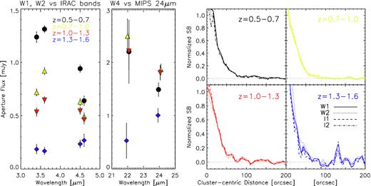
Fluxes measured in 100 arcsec apertures in the WISE W1, W2, W3, IRAC 3.6 |$\, \mu$|m and 4.5 |$\, \mu$|m, and MIPS 24 μm bands. Different colour symbols denote four redshift bins in which the measurements are made. Whenever applicable, the wavelengths are shifted slightly for clarity. Left: In comparing W1 versus 3.6 |$\, \mu$|m and W2 versus 4.5 |$\, \mu$|m, their flux measurements agree with each other within 15 per cent in all redshift bins. Middle: the measured flux in the W4 band is also in good agreement with the MIPS 24 |$\, \mu$|m band, with a slight tendency towards a higher total flux. Possible reasons for this minor disagreement are discussed in Appendix B and Section 4.2. Right: Normalized surface brightness measured in the WISE W1, W2, W3, IRAC 3.6 |$\, \mu$|m and 4.5 |$\, \mu$|m bands are shown for each redshift bin. All are normalized such that the value is 0.5 at 27.5 arcsec (10 native WISE pixels). Despite the differences in angular resolution, the agreement is excellent at nearly all scales.
The flux errors as shown in Fig. B1 fully account for the uncertainties from Poisson noise and from large-scale fluctuation of sky background (see Section 3.1.3). However, there may be two systematic uncertainties unaccounted for in our error estimate. First, the imaging sensitivity, to a large extent, determines the surface density of sources within a given image including numerous faint sources. Together with the source detection setting (i.e. how aggressively we reject them by masking in the pre-stack image processing), these factors can modulate the precision of sky background determination in a way that has yet to be explored. We plan to investigate this issue thoroughly in the future by comparing the results from different detection settings as well as through simulated images spanning a range of added sky rms noise.
In the right-hand panel of Fig. B1, we show the IRAC and WISE-measured radial profiles in all four redshift bins. Evidently, the agreement is excellent in all but the smallest scales where the effects of PSF sizes and angular resolution are expected.
The agreement between the WISE W4 and Spitzer MIPS 24 |$\, \mu$|m bands is also reasonable, as illustrated in the middle panel of Fig. B1. As discussed in Section 4.2, these bands are wide (Δλ = 4–5 μm) and probe a complex portion of the spectrum including several prominent PAH and absorption features. Variations of flux densities up to a factor of a few are expected in individual clusters within a given redshift bin, which certainly contribute to the difference. In addition, a systematic bias may play a role. The 24 μm flux is always lower than the corresponding W4 flux, with the exception of the highest redshift bin where the detection significance is low.
At the wavelength range which the MIPS instrument samples, any data reduction process necessarily includes a more aggressive spatial filtering than is customary at optical and near-IR wavelengths. Median filtering is applied to homogenize the sky background, thereby optimizing for point source detection. The same process unfortunately can eliminate low-level diffuse signals such as that originating from cluster light, leading to a systematic underestimation of both SB and total flux. While such flux loss may be corrected for (through simulations or otherwise) provided that the precise detail of the filtering scheme is known, we wish to stress that spatial filtering can have a nonnegligible impact on both flux and SB measurements.
In this work, we have analysed two different versions of the MAGES data: the official data product and that released as part of the Spitzer Data Fusion project. The latter used a median filter (box with 110 arcsec on a side: D. Shupe, in private communication), much smaller than the former. The identical procedure is followed for both to create image stacks and make flux and SB measurements. We find substantial difference: the use of the aggressively filtered data leads to the smaller angular size of the signal (SB falls to the field level at 50 arcsec compared to 70 arcsec−80 arcsec) and significantly lower fluxes (by ≈60 per cent).
Our analysis shows that the effect is less dramatic (≈15–20 per cent in total flux densities) at 70 μm. Our result is in line with the expectation that the larger filter size used for the 70 μm data to accommodate its much larger beamsize (Table 2) leads to a less exacerbating effect on altering the faint cluster signal.
All in all, our results demonstrate the impressive agreement between the WISE, IRAC, and MIPS measurements, showcasing the potential of the WISE all-sky data to further elucidate the stellar population and star formation activities in galaxy clusters.
APPENDIX C: Testing Herschel/SPIRE stacking
In this appendix, we describe the checks and simulations used to verify the far-IR stacking techniques used in this work. Stacking performed on Herschel/SPIRE maps that are calibrated to have a zero mean should require no additional background noise subtraction or correction for the contribution from the field galaxy population. To verify this, we stacked 53 random cut-outs placed on positions offset from any known cluster. This background stack is compared to a stack of 53 clusters in Fig. C1 and is dominated by (confusion) noise. An appropriate aperture (125 arcsec or |$\sim 1\,$| Mpc at z ∼ 1) recovers a value of zero within the measured uncertainty, indicating that the field population has been correctly ‘zeroed’ out.
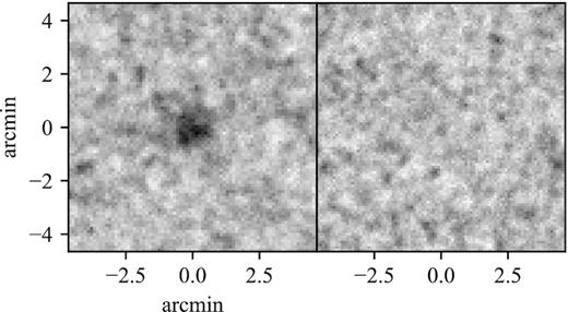
‘total light’ stacking on the SPIRE 250|$\, \mu$|m map centred on 53 1 < z < 1.3 clusters (left) and on 53 random positions offset from the clusters (right).
As a further test, we create simulated maps by injecting artificial clusters composed of point sources arrayed in a normal distribution with a FWHM |$\, = \, 600$| kpc, approximately representing the radial profiles of our real clusters (Section 3.1.6), into a blank map and our real SPIRE 250 |$\, \mu$|m map. The point sources have a uniform, known flux of 3.3 mJy, the typical flux of a massive cluster galaxy (Alberts et al. 2014), below the confusion limit (5.8 mJy, 1σ, at 250 |$\, \mu$|m; Nguyen et al. 2010). We then apply our ‘total light’ stacking technique (Section 3.1.5) to our artificial clusters. The stacking performs the same on the blank and real maps, confirming that our cluster signal is not being boosted by the field population. For the artificial clusters injected in the real map, we recover the total stacked flux within |$10\!-\!15{{\ \rm per\ cent}}$|, within the real bootstrapped uncertainties that are driven by instrument noise, confusion noise, and population variance.
As discussed in Section 3.1.6, when centroiding the real cluster stacks, we found systematic pixel offsets of ∼1–2 pixels that persisted across different cluster sub-sets. Injecting and stacking fake hot pixels into the real maps was used to verify that this offset was not artificially introduced during stacking. A chance offset driven by a few bright, outlier clusters is ruled out by randomly rotating the cut-outs, which eliminates the centroiding offset. This suggests a systematic in the data, perhaps driven by the scan pattern. To be conservative, we randomly rotate all cut-outs during stacking.
In Section 4.3, we discuss an update to the baseline correction first presented in Alberts et al. (2014). In this update, pixels previously chosen at random are now selected from a 2D normal distribution with a FWHM |$\, = \, 600$| kpc, a representative approximation of the extent of the clusters in this study. We test this updated procedure on the simulated maps described above, stacking this time on the known positions of fake cluster members injected into the real map. This test confirms the that updated baseline correction more accurately corrects for flux boosting and clustering signal due to the crowded cluster field and large SPIRE beam out to a radius of |$\sim 1\,$| Mpc, recovering the average flux of the fake cluster sources within the uncertainties. The impact of this update is minimal at |$0.5\,$| Mpc (up to a factor of ∼1.3), but becomes increasingly more important when looking at cluster galaxies at larger radii (up to a factor of ∼2.6 at |$1\,$| Mpc).
