


ABSTRACT
The Vera C. Rubin Observatory Legacy Survey of Space and Time (LSST) will observe several Deep Drilling Fields (DDFs) to a greater depth and with a more rapid cadence than the main survey. In this paper, we describe the ‘DeepDrill’ survey, which used the Spitzer Space Telescope Infrared Array Camera (IRAC) to observe three of the four currently defined DDFs in two bands, centred on 3.6 and 4.5 μm. These observations expand the area that was covered by an earlier set of observations in these three fields by the Spitzer Extragalactic Representative Volume Survey (SERVS). The combined DeepDrill and SERVS data cover the footprints of the LSST DDFs in the Extended Chandra Deep Field–South (ECDFS) field, the ELAIS-S1 field (ES1), and the XMM-Large-Scale Structure Survey field (XMM-LSS). The observations reach an approximate 5σ point-source depth of 2 μJy (corresponding to an AB magnitude of 23.1; sufficient to detect a 10|$^{11} \, \mathrm{M}_{\odot}$| galaxy out to z ≈ 5) in each of the two bands over a total area of |$\approx 29\,$| deg2. The dual-band catalogues contain a total of 2.35 million sources. In this paper, we describe the observations and data products from the survey, and an overview of the properties of galaxies in the survey. We compare the source counts to predictions from the Shark semi-analytic model of galaxy formation. We also identify a population of sources with extremely red ([3.6]−[4.5] >1.2) colours which we show mostly consists of highly obscured active galactic nuclei.
1 INTRODUCTION
Surveys by the Spitzer Space Telescope have proved extremely valuable for finding and characterizing distant galaxies. The redshifting of the peak of stellar emission at |$1.6\, \mu$|m into the Spitzer bands makes them especially sensitive to high-redshift galaxies (e.g. Berta et al. 2007; Stefanon et al. 2015; Cecchi et al. 2019). Spitzer data thus provide a very useful complement to deep surveys in the optical, where the surface density of galaxies is higher, but intrinsically luminous, high-redshift galaxies that are either quiescent or dust-reddened can be outnumbered by lower-redshift, lower luminosity blue galaxies. The Vera C. Rubin Observatory Legacy Survey of Space and Time (LSST; Ivezić et al. 2019) will observe the Southern sky in six optical bands (|$u,\, g,\, r,\, i,\, z$| and y) in about 800 passes (summed over all bands) over 10 yr, to a co-added 5σ depth of AB ≈ 24.4–27.1, depending on band. Within the survey area, there will be several Deep Drilling Fields (DDFs) where observations are repeated more frequently, resulting in both a better sampled cadence, and a deeper co-added final image (AB ≈ 26.2–28.7, depending on band; Brandt et al. 2018; Scolnic et al. 2018). The DDFs will thus become important reference fields for both time domain and ultradeep imaging studies.
We therefore proposed to observe the DDFs that had already been defined by the LSST team in the near-infrared with the Spitzer Space Telescope during its post-cryogenic mission (after the liquid helium cryogen supply for the telescope was exhausted in May 2009). Although only the two shortest wavelength bands of the Infrared Array Camera (IRAC; Fazio et al. 2004a; Carey et al. 2010), at 3.6 and 4.5 μm, continued in operation following the exhaustion of the cryogenic coolant in Spitzer in 2009, their sensitivity was almost unchanged, as was the optical behaviour of the telescope and instrument.
The observations described in this paper supplement an earlier set of observations over smaller areas in these three fields by the Spitzer Extragalactic Representative Volume Survey (SERVS; Mauduit et al. 2012), for which images and catalogues are available from the Infrared Science Archive (IRSA) (a second data release of SERVS, including the data fusion of Vaccari (2015) and deeper Spitzer catalogues is planned). The DeepDrill images are of similar depth to those from SERVS (a 5σ depth of |$\approx 2\, \mu$|Jy in both bands), but cover more than twice the area (≈ 27 deg2 compared to 12 deg2 in these fields covered by SERVS (see Table 1), though SERVS also includes a further 6 deg2 in the Lockman and ELAIS-N1 fields). We also note that deeper warm Spitzer data in the ECDFS field were taken recently as part of the ‘Cosmic Dawn Survey’ (principal investigator: P. Capak). Fig. 1 shows the SERVS-DeepDrill survey in the context of other surveys at ≈3.6 μm. The IRAC image and catalogue data on the three DDFs described in this paper will be made available through the Infrared Science Archive (IRSA).
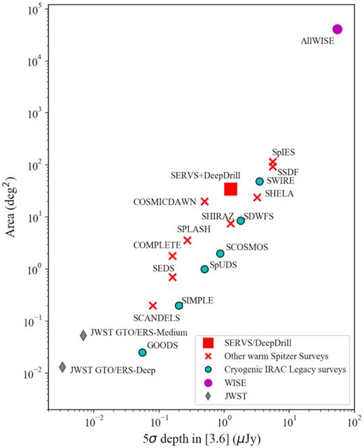
Depth versus area for extragalactic surveys at 3.6 μm. Red crosses indicate surveys taken during the post-cryogenic phase of Spitzer as Exploration Science or Frontier Legacy surveys (surveys which incorporate previous efforts in the same fields have been combined). For comparison, we show surveys taken during the cryogenic mission of Spitzer as cyan circles, WISE mission in magenta, and two Guaranteed Time/Early Release (GTO/ERS) surveys planned for the James Webb Space Telescope in grey. References (top to bottom): AllWISE: Wright et al. (2010), Mainzer et al. (2011); SpIES: Timlin et al. (2016); SSDF: Ashby et al. (2013a); SWIRE: Lonsdale et al. (2003); SERVS+DeepDrill: this paper; SHELA: Papovich et al. (2016); COSMICDAWN: Capak et al. (2016); SDWFS: Ashby et al. (2009); SHIRAZ: Annunziatella et al. (in preparation); SPLASH: Steinhardt et al. (2014); SCOSMOS: Sanders et al. (2007); COMPLETE: Labbe et al. (2016); SpUDS Kim et al. (2011); SEDS: Ashby et al. (2013b); SCANDELS: Ashby et al. (2015); SIMPLE: Damen et al. (2011); GOODS: Dickinson, Giavalisco & GOODS Team (2003); JWST ERS/GTO surveys: Rieke et al. (2019).
Spitzer/IRAC DeepDrill Observations.
| Field name | DeepDrill Field centre | SERVS areaa | DeepDrill | Total areab 3.6 μm | Total areab 4.5 μm | Total areab Both |
|---|---|---|---|---|---|---|
| (J2000) | (deg2) | Observation dates | (deg2) | (deg2) | (deg2) | |
| ES1 | 00:37:48–44:01:30 | 3 | 2015-09-27 to 2016-10-24 | 9.2 | 9.0 | 8.6 |
| XMM-LSS | 02:22:18–04:49:00 | 4.5 | 2015-10-21 to 2016-11-25 | 9.2 | 9.4 | 8.9 |
| ECDFS | 03:31:55–28:07:00 | 4.5 | 2015-05-04 to 2016-12-26 | 9.1 | 9.4 | 8.8 |
a The SERVS field centres differ slightly from the DeepDrill ones, but the SERVS fields are entirely encompassed by the DeepDrill survey.
b Total areas are those covered by the SERVS and DeepDrill data combined.
The scientific motivation for this survey closely followed that for SERVS, namely the study of galaxy evolution as a function of environment from z ∼ 5 to the present, but with the additional feature of the deep and multi-epoch LSST DDF data. The DDFs are expected to be observed throughout the 10 yr duration of the LSST survey, with a cadence as frequent as once every two nights at times of year when the fields are available for observation (Brandt et al. 2018; Scolnic et al. 2018). The time domain adds the ability to detect and obtain light curves of supernovae in distant galaxies (of which we expect ∼104 in the DDFs; LSST Science Collaboration et al. 2009), and to allow the study of AGN flares, tidal disruption events, and other variable phenomena. The Spitzer data provide information on the properties of host galaxies of supernovae and other transients and help to identify and classify AGN, and, indeed, SERVS has already proved useful for these types of investigations (Lunnan et al. 2014; Falocco et al. 2015; Chen et al. 2018). In conjunction with other data at optical and shorter near-infrared wavelengths, the Spitzer survey in these fields will enhance the study of the host galaxies of supernovae and AGN through improved estimates of stellar mass, star formation history, and reddening (Pforr, Maraston & Tonini 2013).
Medium-depth surveys with warm Spitzer covering areas ∼10–100 deg2 have proven very valuable for both studies of individual rare objects (with comoving densities ∼10−5 to 10−8 Mpc−3), and statistical studies of populations including luminous AGN and quasars (∼100 deg−2 in such surveys), galaxy clusters (∼10 deg−2) and ultraluminous dusty star-forming galaxies (∼1000 deg−2). Examples from SERVS include gravitational lenses, Lyman-α nebulae (Marques-Chaves et al. 2018, 2019) and galaxy clusters at z ∼ 0.3–2 (Nantais et al. 2016, 2017; Delahaye et al. 2017; Foltz et al. 2018; Chan et al. 2019; Pintos-Castro et al. 2019; Old et al. 2020; van der Burg et al. 2020).
SERVS has proven particularly valuable for the identification of the host galaxies of radio sources. These galaxies typically have high stellar masses, and are bright in the IRAC bands, with >95 per cent of faint radio sources identified in SERVS (e.g. Luchsinger et al. 2015; Whittam et al. 2015; Mahony et al. 2016; Ocran et al. 2017, 2020a; Singh et al. 2017; Cotton et al. 2018; Prandoni et al. 2018; Ishwara-Chandra et al. 2020). The small population of infrared-faint radio sources (IFRS) that are unidentified, or very faint, in the IRAC bands seem to represent a population of dust-reddened, high-z radio-loud AGN (Norris et al. 2011; Herzog et al. 2014; Maini et al. 2016).
Dusty star-forming galaxies detected in the mm/submm with positions from ALMA can often be identified with faint IRAC sources, allowing better understanding of their stellar masses and extinctions (Simpson et al. 2014; Gómez-Guijarro et al. 2019; Leung et al. 2019; Patil et al. 2019; Dudzevičiūtė et al. 2020; Ocran et al. 2020a, b). Other uses include obtaining constraints on stellar masses and ages of galaxies in overlapping deep spectroscopic surveys (Calabrò et al. 2017; Thomas et al. 2017; Khusanova et al. 2020), studying cosmic background radiation (Mitchell-Wynne et al. 2016) and exploiting fields suitable for deep multiconjugate adaptive optics observations of distant galaxies (Lacy et al. 2018).
The DDFs have garnered significant observational resources from other telescopes, from the radio and far-infrared through to the X-ray. A list of the large-area (|$\gt 1\, {\rm deg}^2$|) surveys in the DDFs may be found in Table 2 (see also table 1 of Chen et al. 2018), and their coverages are illustrated in Figs 2–4. In the X-ray, the XMM-SERVS survey (Chen et al. 2018) is covering the original SERVS areas in ES1, XMM-LSS and ECDFS. The optical data are less homogeneous, including data from Hyper Suprime-Cam (HSC; Aihara et al. 2018; Ni et al. 2019), the Dark Energy Survey (DES; Abbott et al. 2018), and the ESO ESIS and VOICE surveys (Berta et al. 2006; Vaccari et al. 2016), however, as all three fields will be targeted for deep LSST observations this is not a major concern. In the near-infrared, the VISTA VIDEO survey (Jarvis et al. 2013) covers the whole SERVS area, and is supplemented by VEILS (Hönig et al. 2017) which covers the DES fields that are repeatedly observed to find supernovae and other time-domain phenomena (hereafter the DES DDFs). The fields are covered by the SWIRE survey in the mid-infrared (Lonsdale et al. 2003), and the HerMES survey in the far-infrared (Oliver et al. 2012). In the radio, existing deep surveys from the ATCA (ATLAS) (Franzen et al. 2015), GMRT (Smolčić et al. 2018), and LoFAR (Hale et al. 2019) cover a significant fraction of the fields. The MIGHTEE survey with MeerKAT, currently underway, will image the inner regions of all three fields even more deeply at 0.9–1.7 GHz (Jarvis et al. 2016).
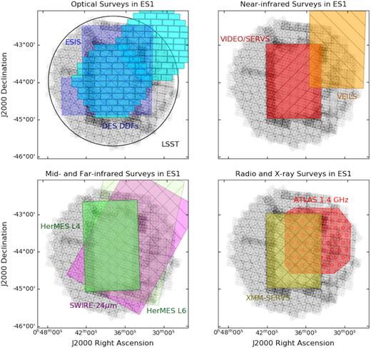
The footprints of multiwavelength surveys on the ELAIS-S1 field (see Table 2 for survey references), superimposed on a greyscale of the IRAC 4.5 μm coverage. Upper left: optical surveys (the DES DDFs are shown in cyan with rectangles indicating the individual chips, the ESIS survey in mauve with cross-hatches, and the LSST footprint is shown as a black circle); upper right, near-infrared surveys (VIDEO in red, left hatched and VEILS in orange, right-hatched). Lower left, 24 μm coverage from SWIRE in magenta and far-infrared coverage in HerMES in green (the L4 data are deeper than the hatched L6 data); lower right: the X-ray XMM-SERVS coverage in yellow, cross-hatched and the ATLAS radio survey in red, with circular hatches.
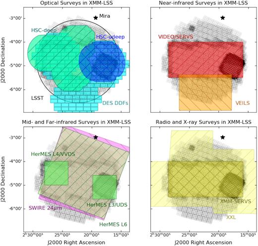
The footprints of multiwavelength surveys on the XMM-LSS field (see Table 2 for survey references), superimposed on a greyscale of the IRAC 4.5 μm coverage. Upper left: optical surveys (the LSST footprint is shown as a black circle, the DES DDFs are in cyan with rectangles indicating the individual chips, the HSC-deep survey is in green with left hatches, the HSC-ultradeep in blue with cross-hatching). Upper right: near-infrared surveys (VIDEO in red, left hatched and VEILS in orange, right-hatched). Lower left: 24 μm coverage from SWIRE in magenta and far-infrared coverage from HerMES in green (the L3 data are the deepest, L4 less deep and L6 the shallowest). Bottom right: X-ray surveys – the XXL survey coverage is shown in light yellow, left-hatched and the XMM-SERVS survey in dark yellow, cross-hatched). The position of the infrared-bright, variable star Mira (K ≈ −2.2) is indicated with the black star symbol.
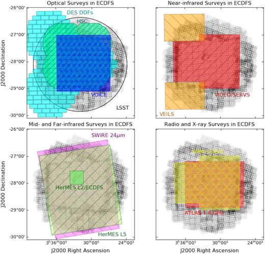
The footprints of multiwavelength surveys on the ECDFS field (see Table 2 for survey references), superimposed on a greyscale of the IRAC 4.5 μm coverage. Upper left: optical surveys (the LSST footprint is shown as a black circle, the DES DDFs are in cyan with rectangles indicating the individual chips, the HSC-deep survey in is green with left hatches, and the VOICE survey is in blue with circular hatches). Upper right: near-infrared surveys (VIDEO in red, left hatched and VEILS in orange, right-hatched); lower left: 24 μm coverage from SWIRE in magenta and far-infrared coverage in HerMES in green (the L2 data are deeper than the hatched L6 data), and lower right: the X-ray XMM-SERVS coverage in yellow, cross-hatched and the ATLAS radio survey in red, with circular hatches.
Other surveys (>1deg2) in the DeepDrill fields.
| Survey | Field(s) | Bands/wavelengths/energies | Overlap area | Depth‡ | Reference |
|---|---|---|---|---|---|
| (deg2) | |||||
| XMM-SERVS | ECDFS, XMM-LSS, ES1 | 0.5-10 keV | 13 | |$1.7 \times 10^{-15}{\rm erg\, cm^{-2} s^{-1}}$| (0.5-2 keV) | Chen et al. (2018) |
| XXL | XMM-LSS | 0.5-10 keV | 8 | |$5 \times 10^{-15}{\rm erg\, cm^{-2} s^{-1}}$| (0.5-2 keV) | Pierre et al. (2016) |
| DEVILS | ECDFS, XMM-LSS | 3750-8850 Å | 4 | Spectroscopic, Y < 21.2 | Davies et al. (2018) |
| ESIS | ES1 | B, V, R | 4.5 | Vega magnitude ≈25 | Berta et al. (2006) |
| VOICE | ECDFS | u, g, r, i | 8 | AB magnitude ≈26 | Vaccari et al. (2016) |
| DES (DR1) | ES1, XMM-LSS, ECDFS | g, r, i, z | 28 | |$AB=25.1,\, 24.8,\, 24.2,\, 23.4,\, 22.2^{\Dagger \Dagger}$| | Abbott et al. (2018) |
| HSC (DR1) | XMM-LSS | g, r, i, z, y | ≈6 | iAB ≈ 26.5–27.0§ | Aihara et al. (2018) |
| HSC (Ni et al.) | ECDFS | g, r, i, z | 5.7 | AB ≈ 25.9, 25.6, 25.8, 25.2 | Ni et al. (2019) |
| SWIRE | ECDFS, XMM-LSS, ES1 | 3.6, 4.5, 5.8, 8.0, 24, 60, 160 μm | 27 | various depths | Lonsdale et al. (2003) |
| OzDES | ES1, XMM-LSS, ECDFS | Spectroscopic; 370-880 nm | 17 | rAB ≈ 23 | Childress et al. (2017) |
| PFS | XMM-LSS | Spectroscopic; 380-1260 nm | 6 | JAB ≈ 23.4 | Takada et al. (2014) |
| VIDEO | ECDFS, XMM-LSS, ES1 | (Z)*, (Y)*, J, H, Ks | 13 | (25.7), (24.6), 24.5, 24.0, 23.5 | Jarvis et al. (2013) |
| VEILS | ECDFS, XMM-LSS, ES1 | |$J,\, K_{s}$| | ≈6 | 25.5, 24.5 | Hönig et al. (2017) |
| HerMES | ECDFS, XMM-LSS, ES1 | 250, 350, 500 μm | 27 | ∼25mJy§ | Oliver et al. (2012) |
| ATLAS | ECDFS, ES1 | 1.4 GHz | 6.3 | 14–17μJy | Franzen et al. (2015) |
| GMRT | XMM-LSS | 610 MHz | 8 | |$\approx 1\,$|mJy | Smolčić et al. (2018) |
| LoFAR | XMM-LSS | 120–168 MHz | 9 | 1.4 mJy | Hale et al. (2019) |
| MIGHTEE | ECDFS, XMM-LSS, ES1 | 900–1670 GHz** | 16.6 | 2μJy | Jarvis et al. (2016) |
Notes. ‡ Typical source detection limit (≈5σ).
* ECDFS was only observed in J, H and Ks.
** A smaller area survey (4 deg2) will also be carried out at 2-4 GHz in ECDFS.
§ The XMM-LSS field of the HSC survey contains one ultradeep pointing and three deep ones, so the depth varies with position.
‡‡ 10σ magnitude limits from Abbott et al. (2018) +0.75 to convert to 5σ; note that there is significant overlap between DeepDrill and the DES Deep Drilling fields (see Figs 2–4, which, when the data are co-added, will be significantly deeper than the main survey).
§ Hurley et al. (2017).
Vaccari (2015) combined SERVS data with catalogues of optical and near-infrared photometry that were available at the time in all five SERVS fields, and Pforr et al. (2019) used these catalogues to derive photometric redshifts for ≈4 million galaxies. Furthermore, the Herschel Extragalactic Legacy Project has incorporated SERVS data within their workflows to produce multiwavelength catalogues and extract more accurate FIR/SMM fluxes to study the dust properties of infrared galaxies over cosmic time (Vaccari 2016; Hurley et al. 2017; Małek et al. 2018; Shirley et al. 2019). For very challenging applications, such as identifying rare sources, and obtaining photometric redshifts accurate enough to study environments, more accurate photometry that allows for the difference between the relatively large Spitzer point spread function and overlapping ground-based surveys in the near-infrared or optical is needed. This more refined photometry requires the application of forced photometry techniques such as The tractor (Lang, Hogg & Mykytyn 2016), and has been successfully used in the XMM-LSS field (Nyland et al. 2017), with the remaining SERVS/DeepDrill fields to follow. The improved photometry and photometric redshifts from it enable the accurate estimation of environmental parameters for galaxies out to at least z ∼ 1.5 (Krefting et al. 2020). The tractor photometry in XMM-LSS was also used to obtain photometric redshifts for X-ray AGN in the XMM-SERVS survey (Chen et al. 2018).
This paper is structured as follows: Section 2 describes the observations, Section 3 the processing of the image data and tests to assess the quality of the astrometric and photometric calibration. Section 4 describes the image and catalogue data products to be included in the release. In Section 5, we present an overview of the galaxy population in DeepDrill, including colours and source counts, and also highlight sources with very red [3.6]−[4.5] colours found in the survey. Section 6 contains a short summary.
2 OBSERVATIONS
We were awarded time to perform a survey of three of the four LSST DDFs that have been defined at the time of writing:1 the ELAIS-S1 field (ES1), the XMM-Large-Scale Structure Survey field (XMM-LSS) and the Extended Chandra Deep Field-South field (ECDFS). The fourth DDF identified by LSST, the COSMOS field, has deep coverage (to 5σ depth of |$\approx 0.3\, \mu$|Jy in both bands) in the inner 2 deg2 from several Spitzer surveys (Sanders et al. 2007; Steinhardt et al. 2014; Ashby et al. 2018). There is also a wider survey (SHIRAZ; Annunziatella et al. in preparation), to a similar depth as SERVS/DeepDrill that covers an additional ≈ 2 deg2 outside of the central area to overlap with the Hyper Suprime-Cam Deep Survey (Aihara et al. 2018).
The central areas of all three of our fields were observed as part of SERVS (Mauduit et al. 2012) during the early months of the post-cryogenic Spitzer mission (2009-07-28 to 2011-03-06). The DeepDrill Survey (Program ID 11086, PI: Lacy) was observed between 2015-05-04 and 2016-12-26 (Table 1). The DeepDrill observations followed the SERVS Astronomical Observation Request (AOR) construction, with each AOR making up a square tile of nine pointings, each pointing consisting of six repeats of 100s frames dithered using the IRAC small cycling dither pattern.2 The use of Fowler sampling in the IRAC detectors (Fazio et al. 2004b) means that the 100 s frame time corresponds to a little less than 100s integration on sky: 93.6 s at 3.6 μm and 96.8 s at 4.5 μm. The fields were imaged in two epochs to facilitate rejection of asteroids, with a targeted depth of 12 frames. Due to scheduling constraints, the time separation of the two epochs was non-uniform, ranging from a few weeks to ∼1 yr. The spatial coverage is also non-uniform. Areas around the edges of the SERVS fields in particular received additional coverage, and some outlying regions did not receive the full coverage. Fig. 5 shows the distribution of coverage in each field. The area in each band with a coverage of 9 or more 100-second frames (i.e. with >87 per cent of the sensitivity of the nominal coverage of 12 frames), and the area with coverage of 9 or more in both bands at the same position are listed in Table 1 (the area with both bands is slightly smaller as the two IRAC detectors are offset). We encourage users with a need for uniformity in depth to make use of the supplied coverage maps.
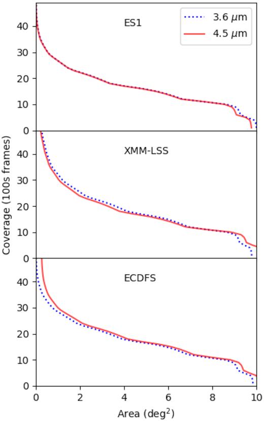
Area of each field as a function of coverage in units of IRAC image frames of 100 s duration. The distribution for the 3.6 μm band is shown as the blue dotted line, and that for the 4.5 μm band as the continuous red line. The small areas of very high (>50) frame coverage in XMM-LSS and ECDFS result from the inclusion of data from earlier deep surveys in these fields, as detailed in Section 3.
The survey was designed such that source confusion only becomes significant near the nominal flux density limit of the survey, where there are about 30 beams per source, the typical value at which source confusion becomes significant (Condon et al. 2012). In Appendix A, we show how the confusion noise is expected to vary with depth of coverage in the survey, including both confusion from randomly distributed sources and an additional term due to galaxy clustering. To more accurately extract faint source parameters from the deepest parts of the survey we recommend PRF fitting of sources and their near-neighbours, which can be further improved by using a prior from a higher resolution survey of similar or greater depth.
3 DATA ANALYSIS
3.1 Image processing
Data processing of the DeepDrill data was similar to that carried out for the SERVS data set (Mauduit et al. 2012), using a data cleaning pipeline derived from processing SWIRE and COSMOS data (Lonsdale et al. 2003; Sanders et al. 2007). The processing began with the Corrected Basic Data (CBCD) frames from the Spitzer Science Center (basic calibrated data frames with corrections for common artefacts, see Lowrance et al. 2016). A refined dark frame for each AOR was constructed after identifying and masking astronomical sources in the data and subtracted from each individual frame in the AOR. Hot pixels in the 4.5μm data were masked, and the column pulldown correction provided in the CBCD was improved (see Lowrance et al. 2012). The images were then rectified to a common background level corresponding to the mean background during the observations. Further corrections were made for latent images on a frame-by-frame basis, as these are particularly prevalent in warm mission data. The data were then mosaicked using mopex (Makovoz, Khan & Masci 2006) (see table 3 of Mauduit et al. 2012, for the parameters used).
A pointing issue was found and corrected in the ES1 field, where the pointing refinement task in the Spitzer data processing pipeline failed for four of the AORs in the South of the field. We also found that we needed to correct the photometric calibration of the SERVS data in ES1, which was taken early in the post-cryogenic mission, while the instrument performance was still being characterized and before the final array temperatures had been set. This was done by comparing the fluxes of sources in the overlap between the SERVS and DeepDrill data sets, and applying the measured offsets to the SERVS data (1.04 at [3.6] and 0.98 at [4.5]). The ES1 data are thus all on the final warm mission calibration. Following Mauduit et al. (2012), the ≈1 deg2 in the southwestern part of the XMM-LSS field that was taken during the cryogenic mission as part of the SpUDS programme (Kim et al. 2011) was included in the final images. The calibrations of these data are the same as those of the DeepDrill data to within 1 per cent, but the SpUDS data are significantly deeper. Similarly, the central ≈0.5 deg2 of the ECDFS field contains data from the much deeper cryogenic SIMPLE (Damen et al. 2011) and GOODS (Dickinson et al. 2003) programmes. However, in this case we used only a depth of ≈12 frames per sky position to obtain an approximately uniform depth for the survey of that field.
3.2 Astrometric accuracy
We matched the DeepDrill catalogues to Gaia Data Release 2 (DR2; Lindegren et al. 2018). The IRAC pointing is calibrated using 2MASS (Skrutskie et al. 2006), and the pointing refinement pipeline now includes proper motion information to provide positions for epoch J2000 (Lowrance et al. 2016). We therefore used the proper motion information in Gaia to derive positions appropriate for the year 2000 to match to the Spitzer positions. We matched the dual-band DeepDrill catalogues to Gaia using a 1|${_{.}^{\prime\prime}}$|0 match radius. 3 per cent of sources in the DeepDrill survey have counterparts in Gaia DR2. The results are shown in Table 3, where we list the mean systematic offset between Spitzer and Gaia DR2 positions Δ(R.A.) and Δ(Decl.), along with the scatter σ(R.A.) and σ(Decl.), representing the positional accuracy of a typical source in the survey. This scatter is independent of source flux, and is thus probably dominated by the scatter in the pointing refinements of individual frames, which is ≈0|${_{.}^{\prime\prime}}$|3 on an individual CBCD frame (Lowrance et al. 2016). All systematic offsets when averaged over a mosaic are <0.1 arcsec.
IRAC source matches in Gaia DR2: number of matches, mean position offsets,and scatter.
| Field | Matches | Δ(R.A.) | Δ(Dec.) | σ(R.A.) | σ(Dec.) |
|---|---|---|---|---|---|
| (arcsec) | (arcsec) | (arcsec) | (arcsec) | ||
| ES1 | 24375 | 0.07 | 0.00 | 0.24 | 0.22 |
| XMM-LSS | 19712 | −0.04 | 0.02 | 0.23 | 0.21 |
| ECDFS | 23946 | −0.02 | 0.02 | 0.20 | 0.21 |
| Field | Matches | Δ(R.A.) | Δ(Dec.) | σ(R.A.) | σ(Dec.) |
|---|---|---|---|---|---|
| (arcsec) | (arcsec) | (arcsec) | (arcsec) | ||
| ES1 | 24375 | 0.07 | 0.00 | 0.24 | 0.22 |
| XMM-LSS | 19712 | −0.04 | 0.02 | 0.23 | 0.21 |
| ECDFS | 23946 | −0.02 | 0.02 | 0.20 | 0.21 |
3.3 Photometric accuracy
The photometric calibration history of IRAC is given in Carey et al. (2012). The post-cryogenic mission calibration factors were obtained by matching the fluxes of the standard stars to the cryogenic observations, and have an absolute accuracy ≈3 per cent. Some scatter is to be expected, as the ≈1|${_{.}^{\prime\prime}}$|8 IRAC PSF is undersampled by the 1|${_{.}^{\prime\prime}}$|2 pixels, and the sensitivity across each pixel varies as a function of position within the pixel. As most of the sources in DeepDrill are slightly extended, and because any given point in the sky is covered by a large number of observations, this intrapixel sensitivity variation is assumed to average out. Aperture corrections were applied as described in Mauduit et al. (2012), using the values in table 2 of that paper.
As noted in Section 3, some SERVS fields (including ES1) were taken early in the Spitzer warm mission, before the calibration factors were finalized. In SERVS, this issue was dealt with by forcing the flux densities to the same scale as SWIRE. The SWIRE flux densities were based on an early calibration of IRAC, and thus there are significant differences between the calibration of the DeepDrill data (which are based on the final Spitzer post-cryogenic mission calibration) and the original SERVS data in the same fields. Table 4 gives the ratio of the calibration factors derived from comparing the DeepDrill to the SERVS Aperture 2 (3|${_{.}^{\prime\prime}}$|9 diameter) flux densities for sources |$\gt 10\, \mu$|Jy in the same field. The more accurate DeepDrill calibration is preferred.
Differences in the photometric calibration between SERVS and DeepDrill (the DeepDrill calibration is preferred.).
| Field | DeepDrill/SERVS flux ratio | |
|---|---|---|
| 3.6 μm | 4.5 μm | |
| ES1 | 0.95 ± 0.01 | 0.96 ± 0.01 |
| XMM-LSS | 0.96 ± 0.01 | 0.98 ± 0.01 |
| ECDFS | 0.95 ± 0.01 | 0.97 ± 0.01 |
| Field | DeepDrill/SERVS flux ratio | |
|---|---|---|
| 3.6 μm | 4.5 μm | |
| ES1 | 0.95 ± 0.01 | 0.96 ± 0.01 |
| XMM-LSS | 0.96 ± 0.01 | 0.98 ± 0.01 |
| ECDFS | 0.95 ± 0.01 | 0.97 ± 0.01 |
4 DATA PRODUCTS
This section briefly describes the data products from DeepDrill that are available in the data release. These consist of images and two sets of catalogues, single-band catalogues and dual-band catalogues.
4.1 Images
Images were made at a pixel scale of 0|${_{.}^{\prime\prime}}$|60 per pixel (oversampling the PSF width of 1|${_{.}^{\prime\prime}}$|8), and are calibrated in MJy sr−1. This results in a conversion factor from pixel values to μJy of 8.46. Coverage images were made, in units of 100-second IRAC frames, along with uncertainty images. Finally, mask images, showing the location of bright stars in the fields are included, made using the methods described in Mauduit et al. (2012).
4.2 Catalogues
Single-band (3.6|$\, \mu$|m and 4.5|$\, \mu$|m) catalogues were produced using SEx tractor (Bertin & Arnouts 1996). Parameters used are shown in Table 5, note some of these differ from Mauduit et al. (2012), principally to improve background filtering: the background mesh size was changed from 32 to 16 pixels, and the filtersize from five to three. These changes improved the background estimates in regions of scattered light around bright objects. The default convolution filter (2-pixel [1|${_{.}^{\prime\prime}}$|2] FWHM) was used for source detection, along with a weight map (the depth of coverage map was used). Photometric apertures labelled 1–5 corresponded to the SWIRE (Lonsdale et al. 2003) standard apertures with radii 1|${_{.}^{\prime\prime}}$|4, 1|${_{.}^{\prime\prime}}$|9, 2|${_{.}^{\prime\prime}}$|9, 4|${_{.}^{\prime\prime}}$|1 and 5|${_{.}^{\prime\prime}}$|8, respectively, with aperture corrections applied per Mauduit et al. (2012). Uncertainties in the flux densities are from SEx tractor, adjusted to allow for the effects of pixel resampling and detector gain. An additional 3 per cent error is added in quadrature to account for the systematic error in the IRAC flux density scale. The raw output from SEx tractor was filtered to output sources with a signal-to-noise ratio >5 in the SWIRE aperture 2 (3|${_{.}^{\prime\prime}}$|9 diameter). The flag column in the catalogue is a bitwise flag that takes the first and second bit of the SEx tractor flag (bit 1: photometry may be affected by neighbours or bad pixels, and bit 2: the source was blended with a neighbouring object), and adds a further flag bit (3) to indicate that the source is either a bright (K < 12) star, or within the region affected by the halo of a bright star according to the rules in Mauduit et al. (2012). The catalogue columns are listed in Table 6. The star masks used to create this flag are included in the data delivery to the Infrared Science Archive (IRSA). The 3.6|$\, \mu$|m and 4.5|$\, \mu$|m catalogues contain 2.7 and 2.5 million sources, respectively, summed over all three fields.
Source extraction parameters used in SEx tractor.
| Parameter | Value |
|---|---|
| DETECT_MINAREA | 5 |
| DETECT_THRESH | 1.0 |
| DETECT_MINCONT | 0.0005 |
| ANALYSIS_THRESH | 0.4 |
| BACK_SIZE | 16 |
| BACK_FILTERSIZE | 3 |
| BACKPHOTO_TYPE | LOCAL |
| Parameter | Value |
|---|---|
| DETECT_MINAREA | 5 |
| DETECT_THRESH | 1.0 |
| DETECT_MINCONT | 0.0005 |
| ANALYSIS_THRESH | 0.4 |
| BACK_SIZE | 16 |
| BACK_FILTERSIZE | 3 |
| BACKPHOTO_TYPE | LOCAL |
Single band catalogue columns.
| Column(s) | Description | Units |
|---|---|---|
| 1 | Name (J2000 coordinates prefixed by DD1) | – |
| 2 | Right Ascension (ICRS) | Degrees |
| 3 | Declination (ICRS) | Degrees |
| 4-8 | Aperture corrected flux densities in apertures 1–5 | μJy |
| 9 | Isophotal flux density | μJy |
| 10 | SEx tractor Auto flux density | μJy |
| 11–17 | Uncertainties on columns 4-10 | μJy |
| 18 | Kron radius | 0|${_{.}^{\prime\prime}}$|6 pixels |
| 19 | Signal-to-noise ratio | – |
| 20 | Local RMS noise | μJy |
| 21 | Coverage | 100s frames |
| 22 | Flag (see text) | – |
Dual-band catalogues were created by matching the two single-band catalogues produced by SEx tractor with a 0|${_{.}^{\prime\prime}}$|6 matching radius (before applying the 5σ cut) and then applying a 3σ cut for the signal-to-noise ratio of the detection in a 3|${_{.}^{\prime\prime}}$|9 diameter at both 3.6 and 4.5μm. (We considered using the dual-image capability of SE xtractor, but we found that the approach of performing two independent source detection rounds on the individual channels and then merging the results in catalogue space resulted in a more reliable catalogue.) There will thus be objects present in the merged catalogue that are not present in the single-band catalogues (and vice versa). The 3.6 μm positions are given in the catalogue as these correspond to the smallest PSF. Columns are listed in Table 7. The dual-band catalogues in each field contain approximately 800 000 sources, giving a total of 2.4 million sources.
Dual band catalogue columns.
| Column(s) | Description | Units |
|---|---|---|
| 1 | Name (J2000 coordinates prefixed by DD1) | – |
| 2 | Right Ascension (ICRS) | Degrees |
| 3 | Declination (ICRS) | Degrees |
| 4–8 | Aperture corrected flux densities at 3.6 μm in apertures 1–5 | μJy |
| 9–13 | Aperture corrected flux densities at 4.5 μm in apertures 1–5 | μJy |
| 14–23 | Uncertainties in columns 4–13 | μJy |
| 24–25 | Isophotal flux densities at 3.6 and 4.5μm | μJy |
| 26–27 | Uncertainties in columns 24–25 | μJy |
| 28–29 | SEx tractor Auto flux densities at 3.6 and 4.5μm | μJy |
| 30–31 | Uncertainties in columns 28–29 | μJy |
| 32–33 | Kron radii at 3.6 and 4.5μm | 0|${_{.}^{\prime\prime}}$|6 pixels |
| 34–35 | Signal-to-noise ratios at 3.6 and 4.5μm | – |
| 36–37 | Coverage | 100s frames |
| 38–39 | Flags at 3.6 and 4.5μm (see the text) | – |
Multiwavelength catalogues in the centre 3–5 deg2 of each of the DeepDrill fields are in the process of construction (Nyland et al. (in preparation), Nyland et al. 2017). These employ forced photometry with the tractor (Lang et al. 2016), using the ground-based near-infrared VIDEO data as a prior to overcome source blending issues. Recovered IRAC magnitudes from this technique are a good match to the aperture magnitudes in SERVS/DeepDrill (Nyland et al. 2017). These catalogues are not part of the initial DeepDrill data release, but will form part of a subsequent data release.
5 ANALYSIS AND RESULTS
5.1 [3.6]–[4.5] colour as a function of redshift
To show the variation of galaxy colour with redshift in DeepDrill we use the photometric redshifts in XMM-LSS from Krefting et al. (2020). These use tractor-based forced photometry (Nyland et al. in preparation, see also Nyland et al. 2017; Cotton et al. 2018) to obtain redshift estimates for 690,000 sources in the overlap between SERVS and DeepDrill. These photometric redshifts have an uncertainty in z/(1 + z) ≈ 0.03 and outlier fraction 1.5 per cent in the redshift range 0 < z < 1.5. To supplement these photometric redshifts with a smaller, but more accurate, sample of spectroscopic redshifts we matched to the OzDES Data Release 1 (Childress et al. 2017), finding 9623 matches within 1|$^{^{\prime \prime }}$| of the DeepDrill positions (corresponding to ≈0.4 per cent of the galaxies in DeepDrill). The OzDES AGN were specially targeted for monitoring programmes.
In the absence of photometric redshifts (still the case over much of the DeepDrill survey), the [3.6]−[4.5] colour can be used as a crude redshift indicator (Papovich 2008). Fig. 6 shows this colour as a function of redshift. The models (based on Maraston 2005) show that the dip in the [3.6]−[4.5] colour at z ≈ 0.6–0.8 is a strong function of the shape of the spectral energy distribution in the near-infrared, which is itself a strong function of the age and nature of the stellar population. Nevertheless, the spectroscopic and photometric redshifts show that most galaxies follow a fairly tight trend in [3.6]−[4.5] colour as a function of redshift. Galaxies with blue colours (bluer than the blue-dotted line at [3.6]−[4.5] = −0.3 in Fig. 6) are at z ≈ 0.5–0.9, and galaxies with red colours (redder than the red-dotted line corresponding to [3.6]−[4.5] =0.1) are at |$z\stackrel{\gt }{_{\sim }}1.3$|. Also shown in Fig. 6 is the boundary colour commonly used to select AGN candidates from WISE data (Stern et al. 2012) : [3.5]−[4.6] >0.8 in the Vega system, corresponding to [3.6]−[4.5] >0.16 in AB. We also plot the colours and photometric redshifts of submm-selected galaxies from the A2SUDS sample of Dudzevičiūtė et al. (2020) and the locus of the [3.6]−[4.5] colour from their composite SED. The very red colour of the A2SUDS SED in the range |$0.3\stackrel{\lt }{_{\sim }}z\stackrel{\lt }{_{\sim }}0.5$| is due to the strong 3.3μm polycyclic aromatic hydrocarbon (PAH) feature passing through the [4.5] band.
![[3.6]−[4.5] colours of galaxies as a function of redshift (cf. Papovich 2008). The grey dots show the galaxies with photometric redshifts in the XMM-LSS field (Krefting et al. 2020), spectroscopic galaxy targets from the OzDES survey (Childress et al. 2017) (OzDES LRG, ClusterGalaxy, RedMaGiC, BrightGalaxy, Emission Line Galaxy and Photo-z types) are shown as orange dots, AGN_monitoring targets from OzDES are shown as cyan crosses, and A2SUDS submm galaxies with photometric redshifts as magenta crosses. The lines indicate various colour cuts; the ‘blue cut’ (blue dotted line) is the line below which the blue population of Fig. 8(d) is selected; ‘red cut’ (red dotted line) the line above which the red population of Fig. 8(d) is selected. We also include the [3.5]−[4.6] colour cut of Stern et al. (2012) (‘AGN cut’; cyan dashed line), above which candidate AGN dominate in the much shallower WISE survey. Three models based on Maraston (2005) evolutionary synthesis models (see Guarnieri et al. 2019) are shown, a 3 Gyr old dusty star-forming galaxy, a 3 Gyr passive galaxy, and a 100 Myr galaxy. (Note that the 3 Gyr models do not extend beyond z = 2.17, where the age of the Universe is 3 Gyr.) We also plot the composite SED of the A2SUDS submm galaxies from Dudzevičiūtė et al. (2020).](https://oup.silverchair-cdn.com/oup/backfile/Content_public/Journal/mnras/501/1/10.1093_mnras_staa3714/1/m_staa3714fig6.jpeg?Expires=1750388664&Signature=aAAiN4BPxIotF8Ds7uJZk8OosQ5rRmihIYbPGSMSmILZG3m9lyZ0eapUb5A~EKREV-jaZE9HTFjhhFxywG61RSK39ajdeGLmACZxphOOIaPOFjcJBz2Gx3lfFFJbISWEQDfTIrN9rI6NZumu71sH22LEZ7O5VionNTGkyXMmNYTUPK9o1SZyBBYW3HP23QlbcDBN~-Slt1~dDhGdjt2ba3qe3pFGttn5vCNBcKGX3cpgN7GXvD6ERjm4KtZJkbv4-aolIGvBwMtWpJApMNyK5rh7v84sEvSPAxaiI6CgYfi914yRG2SuOvL5X2HdZTB9URJJSe5JRwhQI-pXICkXYg__&Key-Pair-Id=APKAIE5G5CRDK6RD3PGA)
[3.6]−[4.5] colours of galaxies as a function of redshift (cf. Papovich 2008). The grey dots show the galaxies with photometric redshifts in the XMM-LSS field (Krefting et al. 2020), spectroscopic galaxy targets from the OzDES survey (Childress et al. 2017) (OzDES LRG, ClusterGalaxy, RedMaGiC, BrightGalaxy, Emission Line Galaxy and Photo-z types) are shown as orange dots, AGN_monitoring targets from OzDES are shown as cyan crosses, and A2SUDS submm galaxies with photometric redshifts as magenta crosses. The lines indicate various colour cuts; the ‘blue cut’ (blue dotted line) is the line below which the blue population of Fig. 8(d) is selected; ‘red cut’ (red dotted line) the line above which the red population of Fig. 8(d) is selected. We also include the [3.5]−[4.6] colour cut of Stern et al. (2012) (‘AGN cut’; cyan dashed line), above which candidate AGN dominate in the much shallower WISE survey. Three models based on Maraston (2005) evolutionary synthesis models (see Guarnieri et al. 2019) are shown, a 3 Gyr old dusty star-forming galaxy, a 3 Gyr passive galaxy, and a 100 Myr galaxy. (Note that the 3 Gyr models do not extend beyond z = 2.17, where the age of the Universe is 3 Gyr.) We also plot the composite SED of the A2SUDS submm galaxies from Dudzevičiūtė et al. (2020).
In Fig. 7 we plot the [4.5] magnitude against redshift for the sample matched to OzDES, the A2SUDS sample and the galaxies with photometric redshifts (note that the ‘banding’ in the distribution of photometric redshifts is an artefact of the photometric redshift algorithm). Most of the galaxies in the survey have stellar masses between 1010 and |$10^{11} \, \mathrm{M}_{\odot}$|, and galaxies with masses of 10|$^{11} \, \mathrm{M}_{\odot}$| can be detected out to z ≈ 5. As expected, the AGN are red and bright, though it should be noted that around the AllWISE limit of |$\mathrm{ AB}\, \approx \, 19.5$| the counts of red galaxies begin to rapidly exceed those of AGN, making selection of AGN based on [3.6]−[4.5] colour alone highly contaminated at faint magnitudes.
![Magnitude versus redshift in [4.5] (symbols as for Fig. 6). Also plotted are two instances of the 3 Gyr old dusty star-forming galaxy model in Fig. 6 with stellar masses of 10$^{10} \, \mathrm{M}_{\odot}$ and 10$^{11} \, \mathrm{M}_{\odot}$, and a 1 Gyr dusty galaxy model with 10$^{11} \, \mathrm{M}_{\odot}$ from the same library, along with the composite submm galaxy SED from A2SUDS.](https://oup.silverchair-cdn.com/oup/backfile/Content_public/Journal/mnras/501/1/10.1093_mnras_staa3714/1/m_staa3714fig7.jpeg?Expires=1750388664&Signature=MF96XE35ujR1l9lmTXSC-BNSxCgM8AaP94NANFycenSvUohJG3nRryVR0khh50mSIbEup8IQljwHJA2hswemErJ6uowtSUROXVZohZsrpPU9lgmdnPH7oOB8L3Mj7ETrUacJ3d4i0ZzABxkN3Mc8nOWV27MatNR2aG~EumvKxTLf1pO6irkXe6fT-dH38QZTNB9b007xyWaz62-Iv8ccIpPQb9POKBiqoTQ5Jo~g2dJQxdh8B7T~sKhdA4LBgd3qgNT3OKMRcjJui7g8eCRkwhqAmBB8ML4PsmyHGjqs-OGMO~~BPMK1n2xaiG8Kj4Eaw35qM5lEQVwCpByrsQr0tg__&Key-Pair-Id=APKAIE5G5CRDK6RD3PGA)
Magnitude versus redshift in [4.5] (symbols as for Fig. 6). Also plotted are two instances of the 3 Gyr old dusty star-forming galaxy model in Fig. 6 with stellar masses of 10|$^{10} \, \mathrm{M}_{\odot}$| and 10|$^{11} \, \mathrm{M}_{\odot}$|, and a 1 Gyr dusty galaxy model with 10|$^{11} \, \mathrm{M}_{\odot}$| from the same library, along with the composite submm galaxy SED from A2SUDS.
5.2 Source counts
Source counts from Spitzer surveys have been presented in Fazio et al. (2004b), Mauduit et al. (2012), Ashby et al. (2013a), Ashby et al. (2015) and Ashby et al. (2018). We compare the differential counts (number per square degree per magnitude) in the DeepDrill fields (Tables 8 and 9) to the S-CANDELS counts of Ashby et al. (2015) (the deepest of the currently published post-cryogenic mission counts) in Fig. 8. Completeness estimates from Mauduit et al. (2012) were used to correct the counts at AB magnitudes <21.25; at fainter magnitudes we ran a new set of simulations (6000 simulated point sources in each half-magnitude bin) on the DeepDrill ES1 field to improve our estimates of completeness (Fig. 8c). These simulations involved scaling point sources extracted from the mosaics to a known flux density corresponding to the mid-point of the magnitude bin, adding a grid of 6000 of these sources at known positions to the mosaic, and rerunning SExtractor. The resulting catalogues were then matched to the known positions within 1|${_{.}^{\prime\prime}}$|2, and the fraction of recovered sources noted as the completeness value for that bin. These extractions also allowed us to examine possible biases in the recovered flux densities near the flux density limit from both Eddington bias (Eddington 1940) and biases from source confusion resulting in an oversubtracted background. We find significant biases only at the faintest magnitudes – at AB = 22.75 (2.9 μJy) the recovered flux densities are higher than those input by 3 per cent at [3.6] and 5 per cent at [4.5], however, this rises to 15 per cent at [3.6] and 24 per cent at [4.5] at AB = 23.25 (1.8 μJy), consistent with Eddington bias dominating. We thus do not list the counts below AB = 22.75.
![DeepDrill source counts. (a) The 3.6 μm counts: the three sets of points show the completeness-corrected counts from each DeepDrill field. The dot-dashed magenta line shows the mean counts from the S-CANDELS fields (Ashby et al. 2015). The magenta dotted line shows star counts from the UDS field (which is within the DeepDrill XMM-LSS field) from Ashby et al. (2015), using the model from Wainscoat et al. (1992) as refined by Cohen (1993), Cohen (1994), Cohen (1995), and Arendt et al. (1998). (As all three fields have Galactic latitudes of −60° ± 15° these will be representative of the survey as a whole.) The dashed black and green lines show the galaxy counts from the Shark (Lagos et al. 2018, 2019) and galform semi-analytic simulations, respectively, and the dotted red line those from the eagle hydrodynamic simulations. (b) The same for the 4.5 μm counts. (c) the survey completeness as a function of magnitude. (d) Counts for red ([3.6]−[4.5] >0.1) and blue ([3.6]−[4.5] <−0.3) sources separately, with the total [4.5] counts also shown, along with model counts from Shark, galform and eagle.](https://oup.silverchair-cdn.com/oup/backfile/Content_public/Journal/mnras/501/1/10.1093_mnras_staa3714/1/m_staa3714fig8.jpeg?Expires=1750388664&Signature=E2SBx7PvJQ2fQV-zPSMlmFPzfLCDPlxtN6UFd-uSy0wnPTUmbc10GEMLYjK9okgTHw2ctYsH4lvrq7mlmyaG1wmQ4PbkD-jWdvAUPE95HPRS0U45U~qSFcgoRXbXlupfVVWLdRySmVqq87wpsx4tRwIYQ-9En9Y2S5-dBmHzsHDni1YqCCGYsm8pT1QB8QgBPxJvt7RTWCN2ZP1XDwDwuoQJ1N~ncthyJtYQSnlMfK7ivcL88QIkgYmmwbY7J6cN3Zl64PEW3DQ1XGxEfEDnCAIFD-m9BSf98pj6M6Sp6wDA8ekWHas03bQzEbkUPj6Kd~b69KeM9AjYOqWZGOQJ-A__&Key-Pair-Id=APKAIE5G5CRDK6RD3PGA)
DeepDrill source counts. (a) The 3.6 μm counts: the three sets of points show the completeness-corrected counts from each DeepDrill field. The dot-dashed magenta line shows the mean counts from the S-CANDELS fields (Ashby et al. 2015). The magenta dotted line shows star counts from the UDS field (which is within the DeepDrill XMM-LSS field) from Ashby et al. (2015), using the model from Wainscoat et al. (1992) as refined by Cohen (1993), Cohen (1994), Cohen (1995), and Arendt et al. (1998). (As all three fields have Galactic latitudes of −60° ± 15° these will be representative of the survey as a whole.) The dashed black and green lines show the galaxy counts from the Shark (Lagos et al. 2018, 2019) and galform semi-analytic simulations, respectively, and the dotted red line those from the eagle hydrodynamic simulations. (b) The same for the 4.5 μm counts. (c) the survey completeness as a function of magnitude. (d) Counts for red ([3.6]−[4.5] >0.1) and blue ([3.6]−[4.5] <−0.3) sources separately, with the total [4.5] counts also shown, along with model counts from Shark, galform and eagle.
Counts at 3.6 μm and their uncertainties for the three DeepDrill fields, the mean, and those from the simulations.
| AB Mag | Completeness | ES1 | Error | XMM-LSS | Error | ECDFS | Error | Mean | Error | Shark | galform | eagle |
|---|---|---|---|---|---|---|---|---|---|---|---|---|
| 14.25 | 1.0 | 1.586 | 0.032 | 1.4 | 0.04 | 1.331 | 0.044 | 1.453 | 0.02 | 0.444 | 0.521 | – |
| 14.75 | 1.0 | 1.928 | 0.022 | 1.883 | 0.023 | 1.91 | 0.022 | 1.907 | 0.013 | 0.785 | 0.656 | – |
| 15.25 | 1.0 | 2.024 | 0.02 | 2.068 | 0.019 | 2.098 | 0.018 | 2.065 | 0.011 | 1.09 | 0.889 | – |
| 15.75 | 1.0 | 2.185 | 0.016 | 2.157 | 0.017 | 2.229 | 0.016 | 2.191 | 0.009 | 1.387 | 1.164 | – |
| 16.25 | 1.0 | 2.304 | 0.014 | 2.314 | 0.014 | 2.371 | 0.013 | 2.331 | 0.008 | 1.666 | 1.403 | – |
| 16.75 | 1.0 | 2.428 | 0.012 | 2.447 | 0.012 | 2.508 | 0.011 | 2.462 | 0.007 | 1.986 | 1.675 | – |
| 17.25 | 1.0 | 2.613 | 0.01 | 2.611 | 0.01 | 2.675 | 0.009 | 2.634 | 0.005 | 2.282 | 2.023 | 1.642 |
| 17.75 | 1.0 | 2.811 | 0.008 | 2.825 | 0.008 | 2.857 | 0.008 | 2.831 | 0.004 | 2.576 | 2.337 | 2.318 |
| 18.25 | 1.0 | 3.088 | 0.006 | 3.089 | 0.006 | 3.111 | 0.006 | 3.096 | 0.003 | 2.878 | 2.658 | 2.853 |
| 18.75 | 1.0 | 3.427 | 0.004 | 3.42 | 0.004 | 3.425 | 0.004 | 3.424 | 0.002 | 3.170 | 3.018 | 3.320 |
| 19.25 | 0.98 | 3.736 | 0.003 | 3.734 | 0.003 | 3.731 | 0.003 | 3.733 | 0.002 | 3.448 | 3.332 | 3.668 |
| 19.75 | 0.96 | 3.973 | 0.002 | 3.966 | 0.002 | 3.969 | 0.002 | 3.97 | 0.001 | 3.699 | 3.613 | 3.915 |
| 20.25 | 0.95 | 4.132 | 0.002 | 4.13 | 0.002 | 4.132 | 0.002 | 4.131 | 0.001 | 3.917 | 3.846 | 4.111 |
| 20.75 | 0.94 | 4.24 | 0.002 | 4.241 | 0.002 | 4.242 | 0.002 | 4.241 | 0.001 | 4.086 | 4.058 | 4.238 |
| 21.25 | 0.91 | 4.342 | 0.008 | 4.344 | 0.008 | 4.345 | 0.008 | 4.344 | 0.008 | 4.216 | 4.237 | 4.338 |
| 21.75 | 0.87 | 4.433 | 0.008 | 4.429 | 0.008 | 4.435 | 0.008 | 4.432 | 0.008 | 4.323 | 4.404 | 4.417 |
| 22.25 | 0.83 | 4.522 | 0.009 | 4.529 | 0.009 | 4.523 | 0.009 | 4.525 | 0.009 | 4.422 | 4.562 | 4.494 |
| 22.75 | 0.76 | 4.652 | 0.010 | 4.650 | 0.010 | 4.646 | 0.010 | 4.649 | 0.009 | 4.524 | 4.701 | 4.580 |
Note. Counts and errors are expressed as log10(N), where N is the count per square degree per magnitude. The errors are based on Poisson statistics, combined with the uncertainty in the completeness estimates (which dominate at fainter magnitudes).
Logarithmic counts at 4.5 μm and their uncertainties for the three DeepDrill fields, the mean, and those from the simulations.
| AB Mag | Completeness | ES1 | Error | XMM-LSS | Error | ECDFS | Error | Mean | Error | Shark | galform | eagle |
|---|---|---|---|---|---|---|---|---|---|---|---|---|
| 14.25 | 1.0 | 1.419 | 0.04 | 1.289 | 0.045 | 1.332 | 0.043 | 1.35 | 0.022 | 0.297 | 0.085 | - |
| 14.75 | 1.0 | 1.761 | 0.027 | 1.825 | 0.024 | 1.859 | 0.023 | 1.817 | 0.014 | 0.604 | 0.521 | - |
| 15.25 | 1.0 | 1.886 | 0.023 | 1.876 | 0.023 | 1.908 | 0.022 | 1.89 | 0.013 | 0.930 | 0.706 | - |
| 15.75 | 1.0 | 2.016 | 0.02 | 2.037 | 0.019 | 2.079 | 0.018 | 2.045 | 0.011 | 1.24 | 0.919 | - |
| 16.25 | 1.0 | 2.201 | 0.016 | 2.176 | 0.016 | 2.252 | 0.015 | 2.211 | 0.009 | 1.545 | 1.225 | - |
| 16.75 | 1.0 | 2.338 | 0.014 | 2.341 | 0.013 | 2.387 | 0.013 | 2.356 | 0.007 | 1.831 | 1.457 | - |
| 17.25 | 1.0 | 2.5 | 0.011 | 2.508 | 0.011 | 2.577 | 0.01 | 2.53 | 0.006 | 2.149 | 1.803 | 1.370 |
| 17.75 | 1.0 | 2.69 | 0.009 | 2.722 | 0.009 | 2.762 | 0.008 | 2.726 | 0.005 | 2.423 | 2.149 | 2.015 |
| 18.25 | 1.0 | 2.965 | 0.007 | 2.972 | 0.006 | 2.995 | 0.006 | 2.978 | 0.004 | 2.717 | 2.453 | 2.642 |
| 18.75 | 1.0 | 3.258 | 0.005 | 3.263 | 0.005 | 3.269 | 0.005 | 3.263 | 0.003 | 3.012 | 2.776 | 3.097 |
| 19.25 | 0.98 | 3.607 | 0.003 | 3.604 | 0.003 | 3.608 | 0.003 | 3.606 | 0.002 | 3.298 | 3.116 | 3.517 |
| 19.75 | 0.96 | 3.919 | 0.002 | 3.927 | 0.002 | 3.926 | 0.002 | 3.924 | 0.001 | 3.577 | 3.450 | 3.811 |
| 20.25 | 0.95 | 4.131 | 0.002 | 4.131 | 0.002 | 4.137 | 0.002 | 4.133 | 0.001 | 3.829 | 3.755 | 4.025 |
| 20.75 | 0.93 | 4.263 | 0.002 | 4.269 | 0.002 | 4.268 | 0.002 | 4.267 | 0.001 | 4.054 | 4.015 | 4.195 |
| 21.25 | 0.92 | 4.347 | 0.008 | 4.347 | 0.008 | 4.356 | 0.008 | 4.35 | 0.008 | 4.223 | 4.224 | 4.311 |
| 21.75 | 0.89 | 4.424 | 0.008 | 4.419 | 0.008 | 4.427 | 0.008 | 4.423 | 0.008 | 4.331 | 4.394 | 4.394 |
| 22.25 | 0.85 | 4.513 | 0.009 | 4.524 | 0.009 | 4.517 | 0.009 | 4.518 | 0.009 | 4.415 | 4.546 | 4.466 |
| 22.75 | 0.76 | 4.639 | 0.01 | 4.604 | 0.01 | 4.631 | 0.01 | 4.625 | 0.009 | 4.509 | 4.665 | 4.551 |
Note. Counts and errors are expressed as log10(N), where N is the count per square degree per magnitude. The errors are based on Poisson statistics, combined with the uncertainty in the completeness estimates (which dominate at fainter magnitudes).
The DeepDrill counts agree well with the deeper counts from the literature, starting to diverge slightly at AB ≈ 22, probably due to differences in the photometric algorithms used when the significance of the DeepDrill detections drops below |$\approx 10\, \sigma$|, and the source confusion limit is approached. We also constructed counts from the deeper data in the |$\approx 0.45\,$|deg2 of the XMM-LSS field that uses images from the SpUDS survey, verifying that the counts in that area have the same shape as the overall counts to AB ≈ 22.5, beyond which they are more complete, as expected.
To measure the counts in DeepDrill, we used the flux densities within the 3|${_{.}^{\prime\prime}}$|8 diameter aperture (with an aperture correction of 0.736 at [3.6] and 0.716 at [4.5]). This will slightly underestimate the fluxes (and hence the counts) at bright magnitudes (AB ∼ 16–18), where the galaxies may be resolved on scales larger than the aperture (at brighter magnitudes the counts are dominated by stars). A comparison to the counts made with the 8|${_{.}^{\prime\prime}}$|2 diameter aperture (with aperture corrections of 0.920 and 0.905 at [3.6] and [4.5], respectively) shows that the counts in this range are about ≈0.1 dex higher in both bands. Over other magnitude ranges the differences are less than 0.1 dex (except at |$\mathrm{ AB} \stackrel{\gt }{_{\sim }} 21$|, when the higher noise results in more incompleteness in the larger aperture). It is also the case that the aperture corrections are derived from point sources, so both the fluxes and the completeness corrections are strictly incorrect for marginally resolved galaxies. However, the good agreement between the counts from the two apertures with very different aperture corrections argues against this being a significant problem. The counts of Ashby et al. (2015) used a point-source fitting method and agree with ours to within 0.1 dex over the whole magnitude range. The point-source fitting method works better on blended objects, but also can be affected by flux boosting from very low level cosmic rays, whereas our use of SE xtractor will probably lead to slight undercounting at faint magnitudes due to blending near the confusion limit.
We also compare our source counts to two semi-analytic simulations, galform and Shark, and to the Evolution and Assembly of GaLaxies and their Environments (eagle) hydrodynamic simulations. Semi-analytic simulations can generate large samples for easy comparison to surveys like DeepDrill, but require some assumptions to be made regarding the effects of dust attenuation in relation to the geometry of disks and bulges to compute observed fluxes, compared to hydrodynamical simulations, which use 3D radiative transfer to calculate these effects directly.
The galform simulated counts are based on a light-cone specifically built for SERVS. This SERVS light-cone of model galaxies was constructed using the Lagos et al. (2012) galform model variant using the techniques described in Merson et al. (2013).3 The light-cone covers the redshift range 0 < z < 6, has a sky coverage of 18.09 deg2 and contains model galaxies with apparent, dust attenuated magnitudes in the [3.6] band down to 2 μJy (see also Krefting et al. 2020). The Shark simulated light-cone was built from the Shark semi-analytic model of galaxy formation and evolution (Lagos et al. 2018, 2019) to compare with the DeepDrill survey. This light-cone has an area of ≈107.9 deg2, and a flux selection at the [3.6] band |$\gt 0.575\, \mu$|Jy (equivalent to an AB magnitude of 24.5), with the same redshift range of 0 ≤ z ≤ 6.
We computed the predicted number counts from the eagle hydrodynamical simulations (Crain et al. 2015; Schaye et al. 2015) by extracting all galaxies at 0 < z < 8 from their public data base (McAlpine et al. 2016), and particularly their redshift, and apparent [3.6] and [4.5] flux densities (see Camps et al. (2018) for details of how these were computed). To calculate the number counts at a given band, we first calculated the area spanned by the box size of |$100\, \rm Mpc$| projected in the sky (we assume that the width of the box is negligible with respect to the luminosity distance and hence we can assume all galaxies in the box to be at the same redshift). We then calculate the number of galaxies per unit area at each redshift and apparent magnitude bin. We then integrate the latter over redshift to obtain a total number per unit area in each magnitude bin, which we then divide by the width of the magnitude bin to compare to our other measurements. We do this at |$3.6\mu$|m, |$4.5\mu$|m and for subsamples of red and blue IRAC galaxies.
Overall, there is a fair agreement between the models and the observations in the regime where galaxies dominate the observed counts (|$\mathrm{ AB}\stackrel{\gt }{_{\sim }}18$|). At intermediate magnitudes, ≈18-21, the semi-analytic models underpredict the number of galaxies compared to both our counts and those in the literature (by up to a factor of 1.8 in the [3.6] band and 2.2 in the [4.5] band for Shark), but the eagle hydrodynamic simulation does better. At the faint end (AB ≈ 22) the galform model does best, with both Shark and eagle underpredicting the counts. All light-cones contain only the stellar emission of galaxies in the IRAC bands, neglecting warm dust emission from AGNs. Including this may improve the agreement between some of the models and the data.
We also examine the source counts as a function of colour, using the red and blue colour cuts described above to isolate intermediate- (z ≈ 0.7) and high-redshift (|$z\stackrel{\gt }{_{\sim }}1.3$|) galaxies. Fig. 8(d) shows these counts, again compared to the model galaxies. Both the blue and red counts start well above all the model counts (in the case of the blue counts at AB < 18 this is due to stars), with eagle producing the largest fraction of blue galaxies, and Shark the smallest. Both sets of observed counts converge to near-agreement with the Shark simulation at the faint end, but the other models do less well, with both eagle and galform overpredicting the blue counts, and galform also overpredicting the red counts. This suggests that the redshift distribution of the sources is quite different in the three simulations. With increasing number of photometric and spectroscopic redshift for SERVS and DeepDrill, we will be able to compare the redshift distributions of the data and the simulations, which will add another dimension to the tests shown here. A detailed discussion of the galaxy luminosity function and stellar mass function using DeepDrill data will also be presented in future papers.
5.3 Very red objects in [3.6]–[4.5]
In this section, we investigate the population of objects in DeepDrill at extreme red [3.6]−[4.5] colours. Such objects are of interest for both Galactic astronomy, where late-type dwarf stars with strong molecular bands can have extreme [3.6]−[4.5] colours (Leggett et al. 2010), and for extragalactic astronomy, where such [3.6]−[4.5] colours are sometimes found for highly obscured, highly luminous AGNs (Tsai et al. 2015). In Table 10 we list the 19 objects detected in both IRAC bands with a signal-to-noise ratio >3 ([3.6]−[4.5] >1.2) that also have 24 μm coverage in SWIRE (3σ depth |$\approx 100\mu$|Jy; total area of overlap ≈ 30 deg2). 16 of the objects have detections at 24 μm, implying their SEDs continue to rise rapidly in the mid-infrared. These are good candidates for dusty high-z AGN. In Fig. 9 we plot the logarithm of the flux density ratio between 3.6 and 5.8‘μm, S5.8/S3.6, versus the logarithm of the flux density ratio between 4.5 and 8.0‘μm, S8.0/S4.5 for the 15 of these objects that are covered by the SWIRE IRAC 5.8 μm and 8.0 μm observations, and compare to the colours of spectroscopically confirmed AGNs from Lacy et al. (2013). Our very red IRAC objects are redder than nearly all of the confirmed AGNs, but follow the extrapolation of the colour trend of AGN to the red (though fall a little below the selection area of Donley et al. 2012). A few of the very red objects have faint detections in VIDEO (Table 10), for these objects the Ks −[4.5] colours of the sources detected at 24μm are also consistent with AGNs (Messias et al. 2012).
![The distribution of the objects with very red [3.6]−[4.5] colours in mid-infrared colour space for all objects with detections in all four IRAC bands. The black crosses indicate probable AGNs, and the brown dot the likely brown dwarf (DD J033258.21−274143.7). The cyan dots represent the spectroscopically confirmed Spitzer-selected AGNs from Lacy et al. (2013), with the selection criteria of AGN candidates for that paper shown as the blue dotted line. We also show the AGN selection criterion of Donley et al. (2012) as the red dot–dash line. Both infrared AGN selection techniques shown here rely on the warm dust emission from the AGN outshining the stellar emission from the host galaxy, see Lacy & Sajina (2020) for a detailed discussion.](https://oup.silverchair-cdn.com/oup/backfile/Content_public/Journal/mnras/501/1/10.1093_mnras_staa3714/1/m_staa3714fig9.jpeg?Expires=1750388664&Signature=W1BoHz4vA75Y-XGo-vQZ-5BpO8-DohfI5OykCOPSCAf8RI59PJHjJGuiceV76CYboOI8PIoryyXRYhaTXr3JKdgIv1priOEZm0KMGLtQxoAzt10LhLruxJ4VKdXC4fMuLQZvEE7mLwpTQrXGucWqKppdUhzOacnNJap1mLAm5naGCtDRPMgZnaJcP4P8bKvT-bRqrqSvgQSUn5KkpECgiVMu79XkVBYbQuQNWC-eu0aGX1WFj4387FYIu1jCUvVs~ik7YHponJ0BxRI-zXuTmyOMsLnc6N0K5Xzqs10f3pDZ-Hqs1O~apD-eC-9V75XQjfi6UFtJQawYxf~De0h2qA__&Key-Pair-Id=APKAIE5G5CRDK6RD3PGA)
The distribution of the objects with very red [3.6]−[4.5] colours in mid-infrared colour space for all objects with detections in all four IRAC bands. The black crosses indicate probable AGNs, and the brown dot the likely brown dwarf (DD J033258.21−274143.7). The cyan dots represent the spectroscopically confirmed Spitzer-selected AGNs from Lacy et al. (2013), with the selection criteria of AGN candidates for that paper shown as the blue dotted line. We also show the AGN selection criterion of Donley et al. (2012) as the red dot–dash line. Both infrared AGN selection techniques shown here rely on the warm dust emission from the AGN outshining the stellar emission from the host galaxy, see Lacy & Sajina (2020) for a detailed discussion.
Mid-infrared and radio photometry of the very red sources from DeepDrill with 24 μm coverage in SWIRE. Infrared photometry is from either the Spitzer source list (SSTSL2; Teplitz et al. 2010), this paper, or S-CANDELS, as noted in the Notes column.
| Name | Ks | S3.6 | S4.5 | S5.8 | S8.0 | S24 | S3GHz | Photometric | Notes |
|---|---|---|---|---|---|---|---|---|---|
| (AB) | (μJy) | (μJy) | (μJy) | (μJy) | (μJy) | (mJy) | redshift | ||
| DD J003136.66−432234.9 | – | 1.2 ± 0.7 | 6.3 ± 0.7 | <20 | <20 | <100 | – | – | |
| DD J003441.85−423119.9 | – | 3.8 ± 0.5 | 15.2 ± 0.4 | 81 ± 4 | 250 ± 6 | 1710 ± 80 | – | – | SSTSL2 |
| DD J003449.14−422934.8 | – | 2.0 ± 0.6 | 6.4 ± 0.5 | 42 ± 7 | 104 ± 7 | 230 ± 30 | – | – | This paper |
| DD J003723.88−432554.7 | – | 1.8 ± 0.6 | 6.9 ± 0.5 | 27 ± 7 | 87 ± 7 | 290 ± 30 | – | – | This paper |
| DD J003831.45−440045.2 | 22.39 ± 0.06 | 3.0 ± 0.7 | 10.7 ± 0.6 | 21 ± 3 | 70 ± 6 | 390 ± 80 | – | – | SSTSL2 |
| DD J004411.11−442448.7 | – | 2.9 ± 0.4 | 9.3 ± 0.4 | <20 | – | 577 ± 30 | – | This paper | |
| DD J021821.44−053101.5 | – | 6.9 ± 0.5 | 21.4 ± 1.0 | 125 ± 7 | 248 ± 7 | 1430 ± 30 | <0.4 | 2.02 | |
| DD J022008.87−041819.0 | 21.04 ± 0.02 | 107.6 ± 3.7 | 337.9 ± 5.3 | 997 ± 30 | 2330 ± 70 | 6010 ± 30 | 0.54 ± 0.12 | 2.01 | |
| DD J022017.88−045753.3 | – | 4.8 ± 0.7 | 15.4 ± 1.2 | 28 ± 4 | 90 ± 8 | 290 ± 60 | <0.4 | – | SSTSL2 |
| DD J022050.38−053714.1 | – | 37.0 ± 1.3 | 122.9 ± 2.5 | 380 ± 10 | 1090 ± 30 | 5000 ± 200 | 2.0 ± 0.12 | 2.05 | 5MUSES-033; This paper |
| DD J022228.02−034235.3 | – | 43.1 ± 1.8 | 143.6 ± 4.2 | 320 ± 10 | 870 ± 30 | 1094 ± 240 | <0.4 | 2.34 | This paper |
| DD J032727.28−270621.9 | – | 1.8 ± 0.9 | 9.7 ± 0.6 | <20 | <20 | <100 | <0.15 | – | |
| DD J032857.12−284111.8 | 22.80 ± 0.06 | 16.0 ± 1.2 | 56.6 ± 2.2 | 173 ± 3 | 443 ± 5 | 1730 ± 90 | <0.15 | – | SSTSL2, This paper |
| DD J033029.88−293445.5 | – | 4.5 ± 0.5 | 14.5 ± 0.7 | 59 ± 7 | 198 ± 7 | 680 ± 30 | <0.15 | – | SSTSL2, This paper |
| DD J033053.41−274717.8 | 22.41 ± 0.06 | 11.9 ± 0.8 | 46.7 ± 2.0 | 150 ± 5 | 480 ± 10 | 2010 ± 40 | <0.15 | – | SSTSL2 |
| DD J033258.19−274143.8 | 22.93 ± 0.06 | 1.7 ± 0.5 | 7.3 ± 0.9 | 5.3 ± 2.2 | 6.1 ± 1.8 | <100 | <0.15 | – | S-CANDELS |
| DD J033400.05−283001.9 | – | 2.7 ± 0.5 | 9.2 ± 0.8 | 47 ± 3 | 80 ± 8 | 200 ± 40 | <0.15 | – | SSTSL2 |
| DD J033401.66−265017.0 | – | 24.4 ± 1.0 | 76.3 ± 1.7 | 176 ± 2 | 227 ± 7 | 1000 ± 50 | <0.15 | – | S340MHz =1.2 mJy; SSTSL2, This paper |
| DD J033602.31−284944.2 | – | 3.6 ± 0.4 | 12.8 ± 1.0 | 33 ± 2 | 87 ± 5 | 490 ± 50 | <0.15 | – | SSTSL2 |
The very red AGNs that are detected at 24 μm have some similarities to objects selected on the basis of extremely red |$R-24\, \mu$|m colours in surveys with Spitzer (dust-obscured galaxies or ‘DOGs’; Dey et al. 2008), very red |$r-22\, \mu$|m colours between the Sloan Digital Sky Survey and WISE (Ross et al. 2015) and objects with very red colours between the WISE bands themselves (‘Hot DOGs’; Tsai et al. 2015). These sets of objects are also dominated by AGN emission in the mid-infrared. However, we emphasize that the [3.6]−[4.5] colours of the very red objects presented here are typically more extreme. None of the DOGs, only 11/77 of the red AGN in Ross et al. (2015) and 5/20 of the Hot DOGs have [3.6]−[4.5] colours as red as the very red objects described here.
Three sources are not detected at 24 μm, and are thus less likely to be AGN. One of these (DD J033258.19−274143.8) is in the much deeper coverage of S-CANDELS, and has faint detections at 5.8 and 8.0 μm (Fig. 9). This object was also detected in multiple epochs of archival Hubble Space Telescope (HST) coverage (2004-08-13 using the ACS instrument through the F850LP filter for proposal ID 9500 and 2011-12-30 through F814W for the CANDELS observations, proposal ID 12060). We downloaded the relevant data from the HST archive, and noted that the object has a significant proper motion, moving approximately 0.7 arcsec in R.A. and 0.5 arcsec in Decl. between the two epochs. We therefore tentatively identify this object as a brown dwarf star. With a [3.5]−[4.6] colour of 1.6 in AB magnitudes (2.2 in Vega magnitudes), this places the star in a spectral class approximately at the transition between T and Y-dwarfs (Leggett et al. 2017). We speculate that the remaining two objects that lack a 24 μm detection may also be brown dwarfs.
To further investigate the possibility of an AGN origin for the majority of the very red sources we searched for serendipitously available mid-infrared spectroscopy as well as deep radio continuum data in the DeepDrill fields. For one of the very red sources, DD J022050.38−053714.1 (5MUSES-033), the Spitzer IRS spectrum from the CASSIS data base (Lebouteiller et al. 2011) shows a strong mid-infrared continuum and spectral features consistent with an AGN at its photometric redshift (derived from SWIRE data) of 2.02 (Rowan-Robinson et al. 2013). This source is also detected in the VLA Sky Survey (VLASS; Lacy et al. 2020) with a 3 GHz flux density |$S_{\mathrm{3 GHz}}=2.0\pm 0.2 \,$|mJy. The correspondingly high radio luminosity of |$L_{\mathrm{3 GHz}}=5\times 10^{25}\, {\rm W\, Hz^{-1}}$| is much more consistent with the radio emission being powered by an AGN rather than by star formation (e.g. Kimball et al. 2011). One further source, DD J022008.87-041819.0 is also detected in VLASS with |$S_{\mathrm{3 GHz}}=0.54 \pm 0.2\,$|mJy. Its photometric redshift is 2.01, which implies |$L_{\mathrm{3 GHz}}=1.3\times 10^{25}\, {\rm W\, Hz^{-1}}$|, also more likely to be powered by an AGN than by star formation. In addition to VLASS, we also searched for counterparts in the deep radio surveys with published source catalogues listed in Table 4 (LOFAR, GMRT, and ATLAS). None of the very red sources is detected in these radio surveys. We also searched for counterparts in deep (sub-mJy beam−1 rms sensitivity) commensal 340 MHz data from the VLA Low-band Ionosphere and Transient Experiment (VLITE4; Clarke et al. 2016; Polisensky et al. 2016) that were observed during an ultradeep, single-pointing VLA imaging campaign centred on the Hubble Ultra Deep Field (HUDF) within CDFS at 3 GHz (Alberts et al. 2020, submitted). Of the 12 very red sources in CDFS that fall within the currently imaged portion (spanning a width of 2 deg) of the deep VLITE data, one source (DD J033401.66−265017.0) has a compact counterpart in VLITE with a primary-beam-corrected flux of 1.0 ± 0.3 mJy at a signal-to-noise ratio of 4.8. The lack of detection in VLASS implies a moderately steep spectral index, |$\alpha ^{0.34\, \mathrm{GHz}}_{3.0\, \mathrm{GHz}}\lt -0.9$|. Unfortunately, the source currently lacks a photometric redshift, though assuming it is at z > 1 it is also more likely to be powered by an AGN. Full details on the deep VLITE imaging centred on the HUDF will be presented in a forthcoming study (Polisensky et al. in preparation).
6 SUMMARY
We describe the DeepDrill survey, which images |$\approx 27\,$|deg2 in three of the four pre-defined LSST Deep Drilling fields to a depth of |$\approx 2\, \mu$|Jy. Accuracy in photometric and astrometric calibration is described. We illustrate the use of the [3.6]−[4.5] colour to divide objects into high (z > 1.3) and low (z ∼ 0.7) redshift bins. This property of the [3.6]−[4.5] colour will be particularly valuable for breaking degeneracies in photometric redshift estimates obtained from LSST optical data alone in regions of the DDFs not covered by other deep near-infrared data (e.g. Pforr et al. 2013).
We show that source count data at [3.6] and [4.5] alone can provide useful comparisons to models of galaxy formation. The model and observed counts generally agree well, but a small discrepancy observed at intermediate magnitudes warrants further investigation. These comparisons will be further enhanced when the Spitzer data are fully combined with the other multiwavelength data in the LSST Deep Drilling fields. We are currently working on completing multiband 0.4-4.5μm catalogues using forced photometry in the centres of the fields (defined by the overlap between the DeepDrill and VIDEO surveys). We show that most objects with extremely red [3.6]−[4.5] colours are mostly identifiable as dusty AGNs at z > 1, but we also find one likely T or Y brown dwarf star and two further brown dwarf candidates. Future papers will discuss the stellar masses of galaxies in DeepDrill (Maraston et al. in preparation) and their clustering (van Kampen et al., in preparation).
The 3–5 μm region in the near-infrared is uniquely useful for capturing light from the peak in the stellar SED at rest frame |$\approx 1\mu$|m at z ∼ 1−4. Although new surveys with Spitzer are no longer possible, we expect that the legacy value of the existing survey data sets will last well into the future. When combined with the existing and planned multiwavelength data sets in these fields, the DeepDrill data will be able to help answer fundamental questions about the nature of AGN and galaxy evolution, and its dependence on environment from before Cosmic Noon to the present.
ACKNOWLEDGEMENTS
We would like to thank the referee for a thorough review that significantly improved the paper. We also thank the contributors to the original DeepDrill proposal not listed as coauthors on this paper, including M. Dickinson, I. Prandoni, and L. Spitler, and especially I. Smail for helpful comments and suggestions. This work is based on observations made with the Spitzer Space Telescope, which was operated by the Jet Propulsion Laboratory, California Institute of Technology under a contract with NASA. Support for this work was provided by NASA through an award issued by JPL/Caltech. The National Radio Astronomy Observatory is a facility of the National Science Foundation operated under cooperative agreement by Associated Universities, Inc. WNB acknowledges support from NASA grant 80NSSC19K0961. GW acknowledges support from the National Science Foundation through grant AST-1517863, by HST program number GO-15294, and by grant number 80NSSC17K0019 issued through the NASA Astrophysics Data Analysis Program (ADAP). Support for program number GO-15294 was provided by NASA through a grant from the Space Telescope Science Institute, which is operated by the Association of Universities for Research in Astronomy, Incorporated, under NASA contract NAS5-26555. IRS acknowledges support from the United Kingdom Science and Technology Facilities Council (ST/P000541/1).JA acknowledges financial support from the Science and Technology Foundation (FCT, Portugal) through research grants PTDC/FIS-AST/29245/2017, UIDB/04434/2020 and UIDP/04434/2020. Basic research in radio astronomy at the Naval Research Laboratory is funded through 6.1 Base funding. This research has made use of the NASA/IPAC Extragalactic Database (NED), which is operated by the Jet Propulsion Laboratory, California Institute of Technology, under contract with the National Aeronautics and Space Administration. This work made extensive use of topcat (Taylor 2011) for catalogue matching and analysis.
DATA AVAILABILITY
The data products from the post-cryogenic Spitzer surveys of the three LSST DDFs described here (images, coverage maps, uncertainty images, bright star masks, and single and dual-band catalogues) are available from IRSA (https://irsa.ipac.caltech.edu/data/SPITZER/DeepDrill). These include mosaic images, coverage maps, uncertainty images, and bright star masks. Each field has two single-band catalogues cut at 5σ, and a dual-band catalogue requiring a detection at >3σ at both 3.6 and 4.5 μm. The simulated light-cone catalogue from Shark is also included in the release; its columns are described in Table 11.
Columns in the Shark simulated light-cone catalogue.
| Column(s) | Description | Units |
|---|---|---|
| 1 | ID | – |
| 2 | Right Ascension | Degrees |
| 3 | Declination | Degrees |
| 4 | Redshift | – |
| 5 | Log10(Stellar Mass) | Solar masses |
| 6 | Log10(Star Formation Rate) | Solar masses/year |
| 7 | Half-light radius | Kpc |
| 8 | Bulge-to-Total ratio | – |
| 9–13 | Apparent mag. in u, g, r, i, z | AB |
| 14–17 | Apparent mag. in Y, J, H, K (VISTA) | AB |
| 18 | Apparent mag. in WISE [3.4] | AB |
| 19–20 | Apparent mag. in IRAC [3.6] and [4.5] | AB |
| 21 | Apparent mag. in WISE [4.6] | AB |
| 22–34 | Absolute mag. in the above bands | AB |
Footnotes
See the IRAC Instrument Handbook https://irsa.ipac.caltech.edu/data/SPITZER/docs/irac/iracinstrumenthandbook/
The data are available from https://zenodo.org/record/3568147#.X2utDC9h2L6
VLITE provides data at 340 MHz from a subset of the VLA antennas during regular VLA observations above 1 GHz over a field-of-view (measured at the full-width at half-power of the primary beam) of 5.5 deg2 and a maximum resolution of ∼5 arcsec in the VLA A configuration.
REFERENCES
APPENDIX A: SOURCE CONFUSION IN THE DEEPDRILL SURVEY
To better understand how source confusion affects the DeepDrill survey as a function of depth, and in the presence of source clustering, we make use of some results from studies at other wavelengths. The analytic approach described here, although only approximate, allows us to predict trends in the noise in the survey as a function of depth, and to compare the contributions of random and clustered sources to the confusion noise.
We next approximate the total noise σT as the contribution of instrumental noise, σI (obtainable from the Spitzer Performance Estimation Tool6) and confusion noise, |$\sigma _{\mathrm{T}}=\sqrt{\sigma _{\mathrm{I}}^2+\sigma _{\mathrm{conf}}^2}$|. (With the caveat that the distribution of deflections P(D) is not Gaussian; Herranz, Kuruoğlu & Toffolatti (2004).) By setting D = σT in equation (A1) and solving numerically, we recover σT = 0.41 μJy at [3.6] and 0.51 μJy at [4.5] at the nominal survey depth of 12 × 100 s frames, close to the empirical result from SERVS of |$\sigma _{\mathrm{T}}\approx 0.4\, \mu$|Jy in both the [3.6] and [4.5] bands found from measuring the RMS variation in randomly placed 1|${_{.}^{\prime\prime}}$|9 radius empty apertures (Mauduit et al. 2012). Table A1 shows that as the depth of the survey is increased beyond the nominal depth of 12 frames, σT decreases, but by factors less than the square root of the number of frames, and the contribution of confusion noise becomes dominant. The contribution from clustering is small, but almost constant with depth as it is dominated by bright sources well above the survey limit, so becomes more significant in deeper surveys. Source confusion in very deep IRAC images can be effectively mitigated by PRF subtraction or forced photometry techniques (e.g. Ashby et al. 2015; Nyland et al. 2017) that remove the PRF wings from the images, reducing Ωe and Ωb.
Calculated noise as a function of depth in DeepDrill.
| Depth | σI | σrandom | |$\lt I\gt \sqrt{\Xi}$| | σconf | σT | |||||
|---|---|---|---|---|---|---|---|---|---|---|
| (100 s | (μJy) | (μJy) | |$(\mu$|Jy) | |$(\mu$|Jy) | (μJy) | |||||
| frames) | [3.6] | [4.5] | [3.6] | [4.5] | [3.6] | [4.5] | [3.6] | [4.5] | [3.6] | [4.5] |
| 6 | 0.35 | 0.51 | 0.33 | 0.41 | 0.15 | 0.13 | 0.36 | 0.43 | 0.51 | 0.67 |
| 9 | 0.29 | 0.42 | 0.30 | 0.36 | 0.15 | 0.13 | 0.34 | 0.38 | 0.45 | 0.57 |
| 12 | 0.25 | 0.36 | 0.28 | 0.33 | 0.15 | 0.14 | 0.32 | 0.36 | 0.41 | 0.51 |
| 24 | 0.18 | 0.25 | 0.25 | 0.28 | 0.16 | 0.14 | 0.30 | 0.31 | 0.34 | 0.41 |
| 48 | 0.13 | 0.18 | 0.23 | 0.24 | 0.16 | 0.14 | 0.28 | 0.28 | 0.30 | 0.33 |
| 96 | 0.09 | 0.13 | 0.21 | 0.22 | 0.16 | 0.14 | 0.27 | 0.26 | 0.28 | 0.29 |
Positional accuracy is also affected by source confusion (Hogg 2001). In the case of DeepDrill, however, the low value of α results in the effect of centroid errors due to source blending at the measured ≈30 beams per source being |$\stackrel{\lt }{_{\sim }}$|0|${_{.}^{\prime\prime}}$|1 (Hogg 2001, their fig. 2).
